(ICLR 2025) TabM: Advancing Tabular Deep Learning With Parameter-Efficient Ensembling
See the code📜 arXiv 📚 Other tabular DL projects
This is the official repository of the paper "TabM: Advancing Tabular Deep Learning With Parameter-Efficient Ensembling". It consists of two parts:
paper/README.md.TabReD is a benchmark based on real-world industrial datasets with time-related distribution drifts and hundreds of features, which makes it more challenging than traditional benchmarks. The figure below shows that TabM achieves higher performance on TabReD (plus one more real-world dataset) compared to prior tabular DL methods.
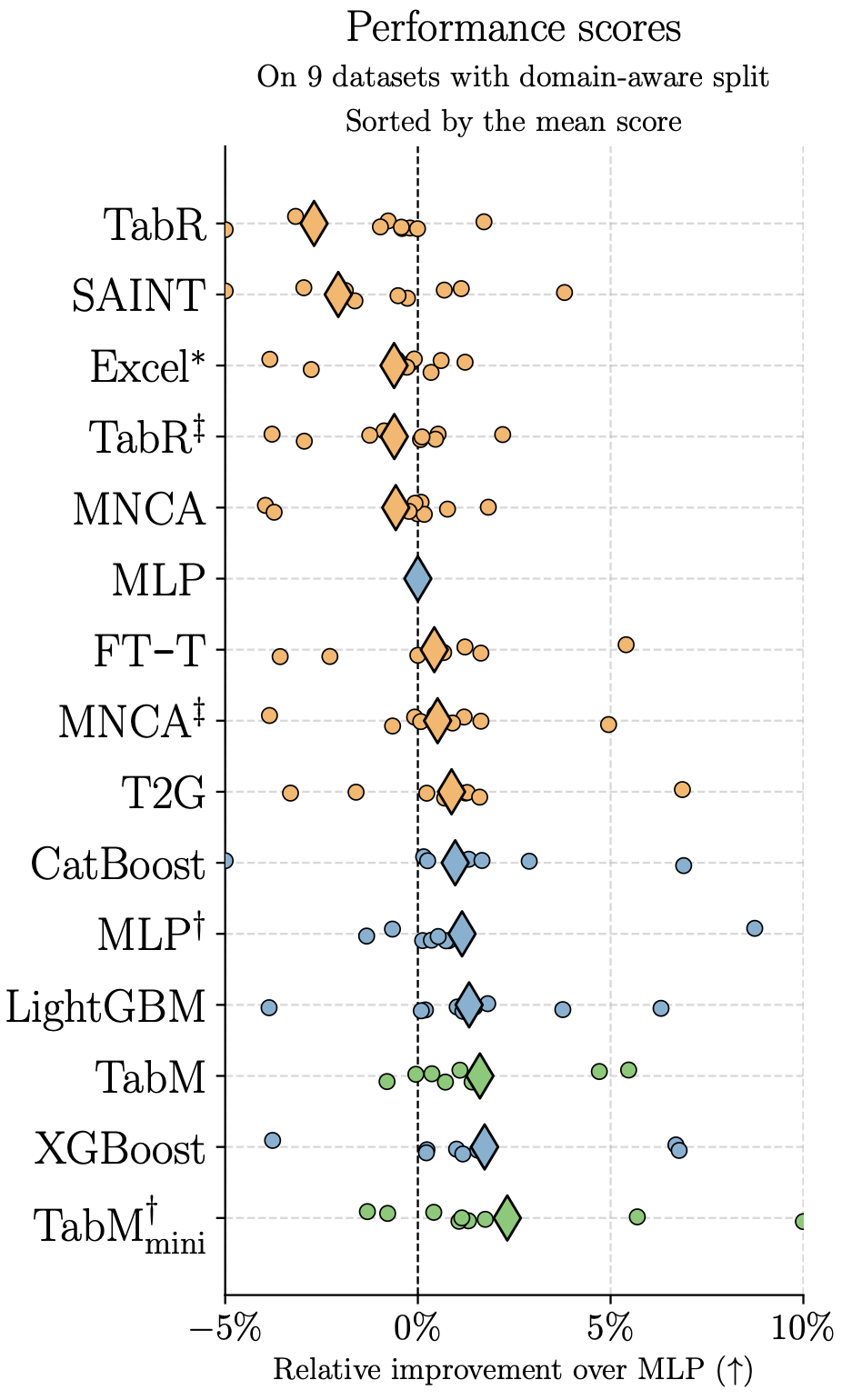
One dot represents a performance score on one dataset. For a given model, a diamond represents the mean value across the datasets.
TabM is a simple and reasonably efficient model, which makes it suitable for real-world applications, including large datasets. The biggest dataset used in the paper contains 13M objects, and we are aware of a successful training run on 100M+ objects, though training takes more time in such cases.
The figure below shows that TabM is relatively slower than MLPs and GBDT, but faster than prior tabular DL methods. Note that (1) the inference throughput was measured on a single CPU thread and without any optimizations, in particular without the TabM-specific acceleration technique described later in this document; (2) the left plot uses the logarithmic scale.
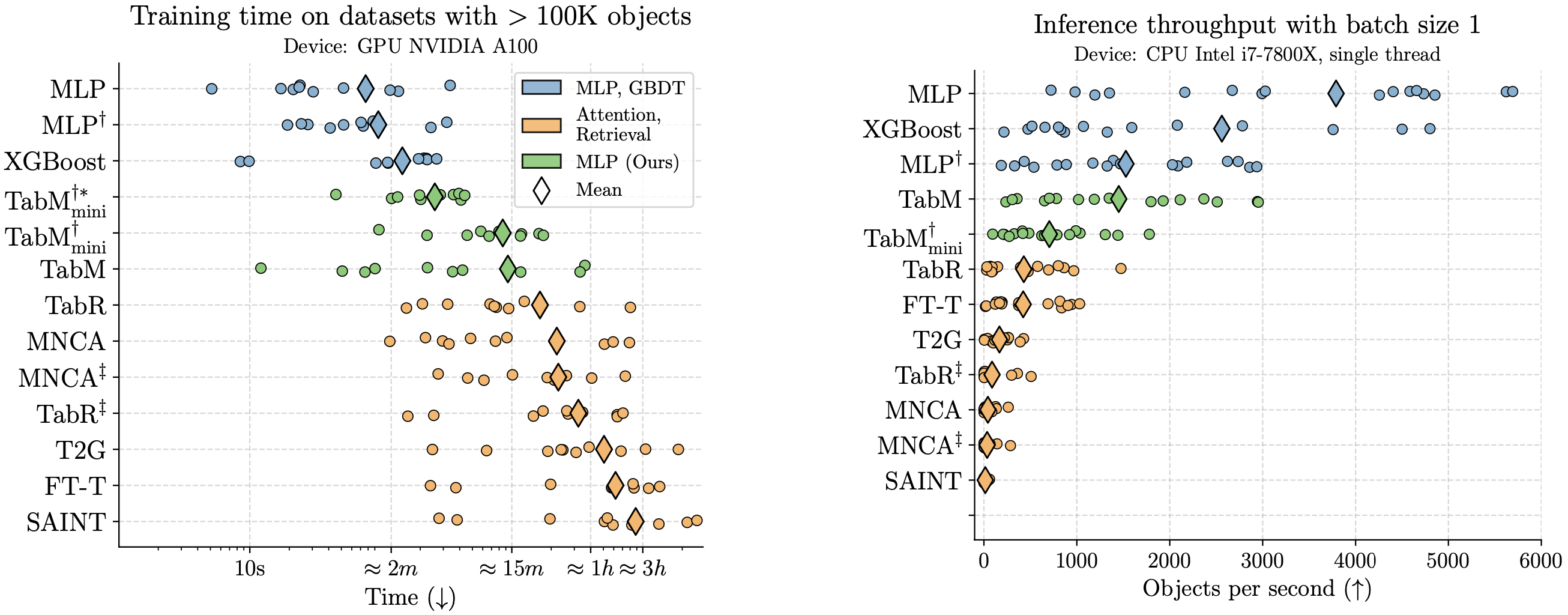
One dot represents a measurement on one dataset. For a given model, a diamond represents the mean value across the datasets. In the left plot, $\mathrm{TabM_{mini}^{\dagger*}}$ denotes $\mathrm{TabM_{mini}^{\dagger}}$ trained with mixed precision and torch.compile.
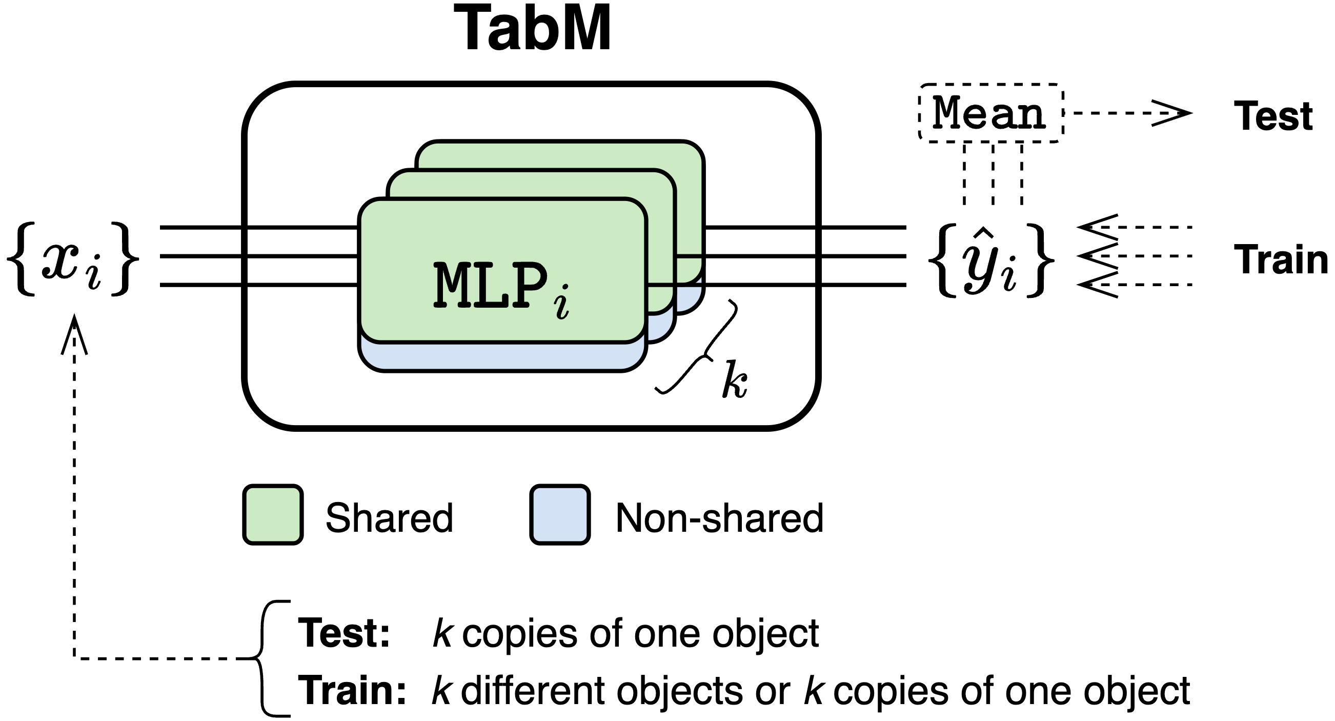
TabM (Tabular DL model that makes Multiple predictions) is a simple and powerful tabular DL architecture that efficiently imitates an ensemble of MLPs. The two main differences of TabM compared to a regular ensemble of MLPs:
[!IMPORTANT] To use TabM in practice and for future work, use the
tabmpackage described below.
The paper-related content (code, metrics, hyperparameters, etc.) is located in the paper/ directory and is described in paper/README.md.
tabm is a PyTorch-based Python package providing the TabM model, as well as layers and tools for building custom TabM-like architectures (i.e. efficient ensembles of MLP-like models).
pip install tabm
This section shows how to create a model in typical use cases, and gives high-level comments on training and inference.
The below example showcases the basic version of TabM without feature embeddings.
For better performance, num_embeddings should usually be passed as explained in the next section.
[!NOTE]
TabM.make(...)used below adds default hyperparameters based on the provided arguments.
import torch
from tabm import TabM

# >>> Common setup for all subsequent sections.
d_out = 1  # For example, one regression task.
batch_size = 256

# The dataset has 24 numerical (continuous) features.
n_num_features = 24

# The dataset has 2 categorical features.
# The first categorical feature has 3 unique categories.
# The second categorical feature has 7 unique categories.
cat_cardinalities = [3, 7]
# <<<

model = TabM.make(
    n_num_features=n_num_features,
    cat_cardinalities=cat_cardinalities,  # One-hot encoding will be used.
    d_out=d_out,
)
x_num = torch.randn(batch_size, n_num_features)
x_cat = torch.column_stack([
    # The i-th categorical features must take values in range(0, cat_cardinalities[i]).
    torch.randint(0, c, (batch_size,)) for c in cat_cardinalities
])
y_pred = model(x_num, x_cat)

# TabM represents an ensemble of k models, hence k predictions per object.
assert y_pred.shape == (batch_size, model.k, d_out)
On typical tabular tasks, the best performance is usually achieved by passing feature embedding
modules as num_embeddings (in the paper, TabM with embeddings is denoted as $\mathrm{TabM^\dagger}$). TabM supports several feature embedding modules from the
rtdl_num_embeddings
package. The below example showcases the simplest embedding module LinearReLUEmbeddings.
[!TIP] The best performance is usually achieved with more advanced embeddings, such as
PiecewiseLinearEmbeddingsandPeriodicEmbeddings. Their usage is covered in the end-to-end usage example.
from rtdl_num_embeddings import LinearReLUEmbeddings

model = TabM.make(
    n_num_features=n_num_features,
    num_embeddings=LinearReLUEmbeddings(n_num_features),
    d_out=d_out
)
x_num = torch.randn(batch_size, n_num_features)
y_pred = model(x_num)

assert y_pred.shape == (batch_size, model.k, d_out)
[!TIP] The implementation of
tabm.TabMis a good example of defining inputs and input modules in TabM-based models.
Assume that you want to change what input TabM takes or how TabM handles the input, but you still want to use TabM as the backbone. Then, a typical usage looks as follows:
from tabm import EnsembleView, make_tabm_backbone, LinearEnsemble


class Model(nn.Module):
    def __init__(self, ...):
        # >>> Create any custom modules.
        ...
        # <<<

        # Create the ensemble input module.
        self.ensemble_view = EnsembleView(...)
        # Create the backbone.
        self.backbone = make_tabm_backbone(...)
        # Create the prediction head.
        self.output = LinearEnsemble(...)

    def forward(self, arg1, arg2, ...):
        # Transform the input as needed to one tensor.
        # This step can include feature embeddings
        # and all other kinds of feature transformations.
        # `handle_input` is a hypothetical user-defined function.
        x = handle_input(arg1, arg2, ...)  # -> (B, D) or (B, k, D)

        # The only difference from conventional models is
        # the call of self.ensemble_view.
        x = self.ensemble_view(x)  # -> (B, k, D)
        x = self.backbone(x)
        x = self.output(x)
        return x  # -> (B, k, d_out)
[!NOTE] Regarding the shape of
xin the linex = handle_input(...):
- TabM can be used as a conventional MLP-like backbone, which corresponds to
xhaving the standard shape(B, D)during both training and inference. This approach is recommended by default due to its simplicity and better efficiency.- There is also an advanced training strategy, where the shape of
xis(B, k, D)during training and(B, D)during inference.The end-to-end usage example covers both approaches.
It is crucial to train the k predictions of TabM indepedendently without averaging them.
In other words, the mean loss must be optimized, not the loss of the mean prediction. The
end-to-end usage example provides a complete reference on how to train TabM.
On inference, to obtain a prediction for a given object, average the k predictions. The exact
averaging strategy depends on the task and loss function. For example, on classification tasks,
probabilities should usually be averaged, not logits. The end-to-end usage example shows how to make predictions with TabM.
example.ipynb provides an end-to-end example of training TabM:
[!TIP] Try and tune TabM before building custom models. The simplicity of TabM can be deceptive, while in fact it is a strong baseline despite using the vanilla MLP as the base model.
This part of the package goes beyond the TabM paper and provides building blocks for creating custom TabM-like architectures, including:
EnsembleView and ElementwiseAffine.Some things are discussed in dedicated sections, and the rest is shown in the examples below.
[!IMPORTANT] Understanding the implementation details of TabM is important for constructing correct and effective TabM-like models. Some of them are discussed later in this section. Other important references:
- The source code of this package, in particular the
TabMmodel and themake_tabm_backbonefunction.- The TabM paper, in particular the $\mathrm{TabM_{mini}}$ paragraph of Section 3.3 (arXiv v3).
Recall that, in conventional MLP-like models, a typical module represents one layer applied to
a tensor of the shape (B, D), where B is the batch size and D is the latent representation
size. By contrast, a typical module in this package:
k layers applied in parallel to k inputs.(B, k, D) representing k inputs (one per layer).Examples:
LinearEnsemble is an ensemble of k independent linear layers.LinearBatchEnsemble is an ensemble of k linear layers sharing most of their weights. Note that
weight sharing does not change how the module is applied: it still represents k layers operating
in parallel over k inputs.EnsembleViewEnsembleView is a special lightweight module doing one simple thing:
(B, D) are turned to tensors of the shape (B, k, D) storing k identical
views of the original tensor. This is a cheap copy-free operation.(B, k, D) are propagated as-is without any changes.The package provides the following efficient MLP ensembles:
MLPBackboneBatchEnsemble (used by $\mathrm{TabM}$)MLPBackboneMiniEnsemble (used by $\mathrm{TabM_{mini}}$)MLPBackboneEnsemble (used by $\mathrm{TabM_{packed}}$)[!NOTE] The difference between creating the above ensembles directly or with the
tabm.make_tabm_backbonefunction is that certain details inmake_tabm_backboneare optimized for TabM. Those details may be useful outside of TabM, too, but this is not explored.
Contrary to TabM, they accept only one three-dimensional input of the shape (batch_size, k, d).
Thus, a user is responsible for converting the input to one tensor (e.g. using embeddings, one-hot
encoding, etc.) storing either k views of the same object or k full-fledged batches. A basic
usage example:
import tabm
import torch
import torch.nn as nn

d_in = 24
d_out = 1
k = 32
model = nn.Sequential(
    tabm.EnsembleView(k=k),
    tabm.MLPBackboneBatchEnsemble(
        d_in=d_in,
        n_blocks=3,
        d_block=512,
        dropout=0.1,
        k=k,
        tabm_init=True,
        scaling_init='normal',
        start_scaling_init_chunks=None,
    ),
    tabm.LinearEnsemble(512, d_out, k=k)
)
x = torch.randn(batch_size, d_in)
y_pred = model(x)
assert y_pred.shape == (batch_size, k, d_out)
This section covers implementation details that are important for building custom TabM-like models.
The order of layers. The most important guideline is that the $k$ different object representations should be created before the tabular features are mixed with linear layers. This follows directly from the $\mathrm{TabM_{mini}}$ paragraph of Section 3.3 of the paper (arXiv V3).
d_in = 24
d = 512
k = 16

# GOOD: collectively, the first two modules create k
# different object representations before the first
# linear layer.
scaling_init = "normal"  # or "random-signs"
good_model = nn.Sequential(
    tabm.EnsembleView(k=k),
    tabm.ElementwiseAffine((k, d_in), bias=False, scaling_init=scaling_init),
    nn.Linear(d_in, d),
    ...
)

# GOOD: internally, LinearBatchEnsemble starts with a
# non-shared elementwise scaling, which diversifies
# the k object representations before the
# linear transformation.
scaling_init = "normal"  # or "random-signs"
                         # or ("normal", "ones")
                         # or ("random-signs", "ones")
good_model = nn.Sequential(
    tabm.EnsembleView(k=k),
    tabm.LinearBatchEnsemble(d_in, d, k=k, scaling_init=scaling_init),
    ...
)

# BAD: the tabular features are mixed before
# the ensemble starts.
bad_model = nn.Sequential(
    nn.Linear(d_in, d),
    tabm.EnsembleView(k=k),
    nn.ReLU(),
    ...
)

# BAD: the k representations are created before the
# first linear transformations, but these representations
# are not different. Mathematically, the below snippet is
# equivalent to the previous one.
bad_model = nn.Sequential(
    tabm.EnsembleView(k=k),
    nn.Linear(d_in, d),
    nn.ReLU(),
    ...
)
Weight sharing. When choosing between torch.nn.Linear (fully sharing linear layers between
ensemble members), tabm.LinearBatchEnsemble (sharing most of the weights) and
tabm.LinearEnsemble (no weight sharing), keep in mind that parameter-efficient ensembling
strategies based on weight sharing (e.g. BatchEnsemble and MiniEnsemble) not only significantly
improve the efficiency of TabM, but also improve its task performance. Thus, weight sharing seems
to be an effective regularization. However, it remains underexplored what is the optimal "amount" of
this regularization and how it depends on a task.
The following code is a reimplementation of tabm.MLPBackboneEnsemble:
k = 32
d_in = 24
d = 512
d_out = 1
dropout = 0.1

model = nn.Sequential(
    tabm.EnsembleView(k=k),

    # >>> MLPBackboneEnsemble(n_blocks=2)
    tabm.LinearEnsemble(d_in, d, k=k),
    nn.ReLU(),
    nn.Dropout(dropout),

    tabm.LinearEnsemble(d, d, k=k),
    nn.ReLU(),
    nn.Dropout(dropout),
    # <<<

    tabm.LinearEnsemble(d, d_out, k=k),
)
MiniEnsemble is a simple parameter-efficient ensembling strategy:
The code below is a reimplementation of tabm.MLPBackboneMiniEnsemble. In fact,
backbone can be any MLP-like model. The only requirement for backbone is to support an arbitrary
number of batch dimensions, since EnsembleView adds a new dimension. Alternatively, one can
reshape the representation before and after the backbone.
d_in = 24
d = 512
d_out = 1
k = 32

# Any MLP-like backbone can be used.
backbone = tabm.MLPBackbone(
    d_in=d_in, n_blocks=2, d_block=d, dropout=0.1
)
model = nn.Sequential(
    tabm.EnsembleView(k=k),

    # >>> MLPBackboneMiniEnsemble
    tabm.ElementwiseAffine((k, d_in), bias=False, scaling_init='normal'),
    backbone,
    # <<<

    tabm.LinearEnsemble(d, d_out, k=k),
)
The following code is a reimplementation of tabm.MLPBackboneBatchEnsemble with n_blocks=2:
k = 32
d_in = 24
d = 512
dropout = 0.1
tabm_init = True  # TabM-style initialization
scaling_init = 'normal'  # or 'random-signs'

model = nn.Sequential(
    tabm.EnsembleView(k=k),

    # >>> MLPBackboneBatchEnsemble(n_blocks=2)
    tabm.LinearBatchEnsemble(
        d_in, d, k=k,
        scaling_init=(scaling_init, 'ones') if tabm_init else scaling_init,
    ),
    nn.ReLU(),
    nn.Dropout(dropout),

    tabm.LinearBatchEnsemble(
        d, d, k=k,
        scaling_init='ones' if tabm_init else scaling_init
    ),
    nn.ReLU(),
    nn.Dropout(dropout),
    # <<<

    tabm.LinearEnsemble(d, d_out, k=k),
)
A random and most likely bad architecture showcasing various layers available in the package:
d_in = 24
d = 512
d_out = 1
k = 16
dropout = 0.1

model = nn.Sequential(
                                         #    (B, d_in) or (B, k, d_in)
    tabm.EnsembleView(k=k),              # -> (B, k, d_in)

    # Most of the weights are shared
    tabm.LinearBatchEnsemble(            # -> (B, k, d)
        d_in, d, k=k, scaling_init=('random-signs', 'ones')
    ),
    nn.ReLU(),                           # -> (B, k, d)
    nn.Dropout(dropout),                 # -> (B, k, d)

    # No weight sharing
    tabm.BatchNorm1dEnsemble(d, k=k),    # -> (B, k, d)

    # No weight sharing
    tabm.LinearEnsemble(                 # -> (B, k, d)
        d, d, k=k
    ),
    nn.ReLU(),                           # -> (B, k, d)
    nn.Dropout(dropout),                 # -> (B, k, d)

    # The weights are fully shared
    nn.Linear(                           # -> (B, k, d)
        d, d,
    ),
    nn.ReLU(),                           # -> (B, k, d)
    nn.Dropout(dropout),                 # -> (B, k, d)

    # No weight sharing
    tabm.ElementwiseAffine(              # -> (B, k, d)
        (k, d), bias=True, scaling_init='normal'
    ),

    # The weights are fully shared
    tabm.MLPBackbone(                    # -> (B, k, d)
        d_in=d, n_blocks=2, d_block=d, dropout=0.1
    ),

    # Almost all the weights are shared
    tabm.MLPBackboneMiniEnsemble(        # -> (B, k, d)
        d_in=d, n_blocks=2, d_block=d, dropout=0.1,
        k=k, affine_bias=False, affine_scaling_init='normal',
    ),

    # No weight sharing
    tabm.LinearEnsemble(d, d_out, k=k),  # -> (B, k, d_out)
)

x = torch.randn(batch_size, d_in)
y_pred = model(x)
assert y_pred.shape == (batch_size, k, d_out)
[!WARNING] The approach discussed below requires full understanding of all implementation details of both the original model and efficient ensembling, because it does not provide any guarantees on correctness and performance of the obtained models.
Assume that you have an MLP-like model, and you want to quickly evaluate the potential of efficient ensembling applied to your model without changing the model's source code. Then, you can create a single-model instance and turn it to an efficient ensemble by replacing its layers with their ensembled versions. To that end, the package provides the following functions:
tabm.batchensemble_linear_layers_tabm.ensemble_linear_layers_tabm.ensemble_batchnorm1d_layers_tabm.ensemble_layernorm_layers_For example, the following code creates a full-fledged ensemble of $k$ independent MLPs:
d_in = 24
d = 512
d_out = 1

# Create one standard MLP backbone.
backbone = tabm.MLPBackbone(
    d_in=d_in, n_blocks=3, d_block=d, dropout=0.1
)

# Turn the one backbone into an efficient ensemble.
k = 32
tabm.ensemble_linear_layers_(backbone, k=k)

# Compose the final model.
model = nn.Sequential(
    tabm.EnsembleView(k=k),
    backbone,
    tabm.LinearEnsemble(d, d_out, k=k),
)
assert model(torch.randn(batch_size, d_in)).shape == (batch_size, k, d_out)
TabM.make allows one to create TabM with the default hyperparameters and overwrite them as needed:
[!NOTE] The default hyperparameters are not "constant", i.e. they depend on the provided arguments.
# TabM with default hyperparameters.
model = TabM.make(n_num_features=16, d_out=1)

# TabM with custom n_blocks
# and all other hyperparameters set to their default values.
model = TabM.make(n_num_features=16, d_out=1, n_blocks=2)
Currently, for the default TabM, the default optimizer is
torch.optim.AdamW(..., lr=0.002, weight_decay=0.0003).
arch_typeTL;DR: by default, use TabM.
'tabm' is the default value and is expected to provide the best performance in most cases.'tabm-mini' may result in a faster training and/or inference without a significant performance
drop, though this option may require a bit more precision when choosing d_block and n_blocks
for a given k. 'tabm-mini' can occasionally provide slightly better performance if the
higher degree of regularization turns out to be beneficial for a given task.'tabm-packed' is implemented only for completeness. In most cases, it results in a slower,
heavier and weaker model.k[!TIP] All the following points about
k, except for the first one, are inspired by Figure 7 from the paper (arXiv v3).
k, consider running independent hyperparameter tuning runs with different,
but fixed values of k. The motivation is that changing k can affect optimal
values of other hyperparameters, which can hinder the hyperparameter tuning process if k is
tuned together with other hyperparameters.k up to a certain threshold can improve performance.
After the threshold, the performance may not improve and can even become worse. This effect is
more pronounced for arch_type='tabm-mini' (not shown in the figure).k (i.e. 24 or 16) and still get
competitive results (though changing k can require retuning other hyperparameters).k, consider increasing d_block or n_block (or both).
The intuition is that, because of the weight sharing, the larger ensemble size may require
larger base architecture to successfully accommodate k submodels.n_blocks=1 should usually be avoided unless you have high budget on hyperparameter tuning.num_embeddingsrtdl_num_embeddings package provides recommendations on hyperparameter
tuning for embeddings.This section provides an overview of initialization-related options that one has to specify when
using API other than TabM.make.
[!NOTE] The extent to which the initialization-related settings affect the task performance depends on a task at hand. Usually, these settings are about uncovering the full potential of TabM, not about avoiding some failure modes.
TabM-style initialization. tabm_init is a flag triggering the TabM-style initialization of
BatchEnsemble-based models. In short, this is a conservative initialization strategy making the $k$
submodels different from each other only in the very first ensembled layer, but equal in all other
layers at initialization. On benchmarks, tabm_init=True showed itself as a better default
strategy. If the $k$ submodels collapse to the same model during training, try tabm_init=False.
Initialization of scaling parameters. The arguments start_scaling_init, scaling_init and affine_scaling_init are all about the same thing in slightly different contexts. TabM uses an
informal heuristic rule that can be roughly summarized as follows: use "normal" if there are
"non-trivial" modules before the TabM backbone (e.g. num_embeddings), and "random-signs"
otherwise. This is not a well-explored aspect of TabM.
Initialization chunks. The arguments like start_scaling_init_chunks or scaling_init_chunks
trigger a heuristic chunk-based initialization of scaling parameters, where the chunk sizes must sum
exactly to the backbone input size (i.e. d_in.) By default, in TabM, the "chunks" are defined
simply as feature representation sizes (see the d_features variable in tabm.TabM.__init__),
which means that, during the initialization, exactly one random scalar will be sampled per feature.
In other contexts, it may be unclear how to define chunks. In such cases, one possible approach is
to start with None and, if needed, try to find a better approach by trial and error.
[!TIP] The general notes provided above will help you in automatic hyperparameter tuning as well.
It the paper, to tune TabM's hyperparameters, the TPE sampler from Optuna was used with 100 iterations on smaller datasets, and 50 iterations on larger datasets. If achieving the highest possible performance is not critical, then 30-50 iterations should result in a somewhat reasonable configuration.
The below table provides the hyperparameter distributions used in the paper. Consider changing them based on your setup and taking previous sections into account, especially if the lower number of iterations is used.
| Hyperparameter | TabM | TabM w./ PiecewiseLinearEmbeddings |
|---|---|---|
k | Const[32] (not tuned) | Same as for TabM |
n_blocks | UniformInt[1, 5] | UniformInt[1, 4] |
d_block | UniformInt[64, 1024, step=16] | Same as for TabM |
lr | LogUniform[1e-4, 5e-3] | Same as for TabM |
weight_decay | {0, LogUniform[1e-4, 1e-1]} | Same as for TabM |
n_bins | N/A | UniformInt[2, 128] |
d_embedding | N/A | UniformInt[8, 32, step=4] |
As shown in Section 5.2 of the paper, one can prune a significant portion of TabM's submodels
(i.e. reduce k) after the training at the cost of a minor performance drop. In theory, there are
more advanced algorithms for selecting the best subset of submodels, such as the
one by Caruana et al.,
but they were not analyzed in the paper. Also, keep in mind that selecting, say, k=8 submodels
after training with k=32 will result in a better model than simply training with k=8.
To explore the package API and docstrings, do one of the following:
make docs.To list all available items without cloning or installing anything, run the following snippet:
uv run --no-project --with tabm python -c """
import tabm

for x in sorted(
    x
    for x in dir(tabm)
    if getattr(getattr(tabm, x), '__module__', None) == 'tabm'
    and not x.startswith('_')
):
    print(x)
"""
61,643 followers · starred Jul 2025
497 followers · starred Jul 2025
70 followers · starred Jun 2025
52 followers · starred Jun 2025
(ICLR 2025) TabM: Advancing Tabular Deep Learning With Parameter-Efficient Ensembling
See the code📜 arXiv 📚 Other tabular DL projects
This is the official repository of the paper "TabM: Advancing Tabular Deep Learning With Parameter-Efficient Ensembling". It consists of two parts:
paper/README.md.TabReD is a benchmark based on real-world industrial datasets with time-related distribution drifts and hundreds of features, which makes it more challenging than traditional benchmarks. The figure below shows that TabM achieves higher performance on TabReD (plus one more real-world dataset) compared to prior tabular DL methods.
One dot represents a performance score on one dataset. For a given model, a diamond represents the mean value across the datasets.
TabM is a simple and reasonably efficient model, which makes it suitable for real-world applications, including large datasets. The biggest dataset used in the paper contains 13M objects, and we are aware of a successful training run on 100M+ objects, though training takes more time in such cases.
The figure below shows that TabM is relatively slower than MLPs and GBDT, but faster than prior tabular DL methods. Note that (1) the inference throughput was measured on a single CPU thread and without any optimizations, in particular without the TabM-specific acceleration technique described later in this document; (2) the left plot uses the logarithmic scale.
One dot represents a measurement on one dataset. For a given model, a diamond represents the mean value across the datasets. In the left plot, $\mathrm{TabM_{mini}^{\dagger*}}$ denotes $\mathrm{TabM_{mini}^{\dagger}}$ trained with mixed precision and torch.compile.
TabM (Tabular DL model that makes Multiple predictions) is a simple and powerful tabular DL architecture that efficiently imitates an ensemble of MLPs. The two main differences of TabM compared to a regular ensemble of MLPs:
[!IMPORTANT] To use TabM in practice and for future work, use the
tabmpackage described below.
The paper-related content (code, metrics, hyperparameters, etc.) is located in the paper/ directory and is described in paper/README.md.
tabm is a PyTorch-based Python package providing the TabM model, as well as layers and tools for building custom TabM-like architectures (i.e. efficient ensembles of MLP-like models).
pip install tabm
This section shows how to create a model in typical use cases, and gives high-level comments on training and inference.
The below example showcases the basic version of TabM without feature embeddings.
For better performance, num_embeddings should usually be passed as explained in the next section.
[!NOTE]
TabM.make(...)used below adds default hyperparameters based on the provided arguments.
import torch
from tabm import TabM

# >>> Common setup for all subsequent sections.
d_out = 1  # For example, one regression task.
batch_size = 256

# The dataset has 24 numerical (continuous) features.
n_num_features = 24

# The dataset has 2 categorical features.
# The first categorical feature has 3 unique categories.
# The second categorical feature has 7 unique categories.
cat_cardinalities = [3, 7]
# <<<

model = TabM.make(
    n_num_features=n_num_features,
    cat_cardinalities=cat_cardinalities,  # One-hot encoding will be used.
    d_out=d_out,
)
x_num = torch.randn(batch_size, n_num_features)
x_cat = torch.column_stack([
    # The i-th categorical features must take values in range(0, cat_cardinalities[i]).
    torch.randint(0, c, (batch_size,)) for c in cat_cardinalities
])
y_pred = model(x_num, x_cat)

# TabM represents an ensemble of k models, hence k predictions per object.
assert y_pred.shape == (batch_size, model.k, d_out)
On typical tabular tasks, the best performance is usually achieved by passing feature embedding
modules as num_embeddings (in the paper, TabM with embeddings is denoted as $\mathrm{TabM^\dagger}$). TabM supports several feature embedding modules from the
rtdl_num_embeddings
package. The below example showcases the simplest embedding module LinearReLUEmbeddings.
[!TIP] The best performance is usually achieved with more advanced embeddings, such as
PiecewiseLinearEmbeddingsandPeriodicEmbeddings. Their usage is covered in the end-to-end usage example.
from rtdl_num_embeddings import LinearReLUEmbeddings

model = TabM.make(
    n_num_features=n_num_features,
    num_embeddings=LinearReLUEmbeddings(n_num_features),
    d_out=d_out
)
x_num = torch.randn(batch_size, n_num_features)
y_pred = model(x_num)

assert y_pred.shape == (batch_size, model.k, d_out)
[!TIP] The implementation of
tabm.TabMis a good example of defining inputs and input modules in TabM-based models.
Assume that you want to change what input TabM takes or how TabM handles the input, but you still want to use TabM as the backbone. Then, a typical usage looks as follows:
from tabm import EnsembleView, make_tabm_backbone, LinearEnsemble


class Model(nn.Module):
    def __init__(self, ...):
        # >>> Create any custom modules.
        ...
        # <<<

        # Create the ensemble input module.
        self.ensemble_view = EnsembleView(...)
        # Create the backbone.
        self.backbone = make_tabm_backbone(...)
        # Create the prediction head.
        self.output = LinearEnsemble(...)

    def forward(self, arg1, arg2, ...):
        # Transform the input as needed to one tensor.
        # This step can include feature embeddings
        # and all other kinds of feature transformations.
        # `handle_input` is a hypothetical user-defined function.
        x = handle_input(arg1, arg2, ...)  # -> (B, D) or (B, k, D)

        # The only difference from conventional models is
        # the call of self.ensemble_view.
        x = self.ensemble_view(x)  # -> (B, k, D)
        x = self.backbone(x)
        x = self.output(x)
        return x  # -> (B, k, d_out)
[!NOTE] Regarding the shape of
xin the linex = handle_input(...):
- TabM can be used as a conventional MLP-like backbone, which corresponds to
xhaving the standard shape(B, D)during both training and inference. This approach is recommended by default due to its simplicity and better efficiency.- There is also an advanced training strategy, where the shape of
xis(B, k, D)during training and(B, D)during inference.The end-to-end usage example covers both approaches.
It is crucial to train the k predictions of TabM indepedendently without averaging them.
In other words, the mean loss must be optimized, not the loss of the mean prediction. The
end-to-end usage example provides a complete reference on how to train TabM.
On inference, to obtain a prediction for a given object, average the k predictions. The exact
averaging strategy depends on the task and loss function. For example, on classification tasks,
probabilities should usually be averaged, not logits. The end-to-end usage example shows how to make predictions with TabM.
example.ipynb provides an end-to-end example of training TabM:
[!TIP] Try and tune TabM before building custom models. The simplicity of TabM can be deceptive, while in fact it is a strong baseline despite using the vanilla MLP as the base model.
This part of the package goes beyond the TabM paper and provides building blocks for creating custom TabM-like architectures, including:
EnsembleView and ElementwiseAffine.Some things are discussed in dedicated sections, and the rest is shown in the examples below.
[!IMPORTANT] Understanding the implementation details of TabM is important for constructing correct and effective TabM-like models. Some of them are discussed later in this section. Other important references:
- The source code of this package, in particular the
TabMmodel and themake_tabm_backbonefunction.- The TabM paper, in particular the $\mathrm{TabM_{mini}}$ paragraph of Section 3.3 (arXiv v3).
Recall that, in conventional MLP-like models, a typical module represents one layer applied to
a tensor of the shape (B, D), where B is the batch size and D is the latent representation
size. By contrast, a typical module in this package:
k layers applied in parallel to k inputs.(B, k, D) representing k inputs (one per layer).Examples:
LinearEnsemble is an ensemble of k independent linear layers.LinearBatchEnsemble is an ensemble of k linear layers sharing most of their weights. Note that
weight sharing does not change how the module is applied: it still represents k layers operating
in parallel over k inputs.EnsembleViewEnsembleView is a special lightweight module doing one simple thing:
(B, D) are turned to tensors of the shape (B, k, D) storing k identical
views of the original tensor. This is a cheap copy-free operation.(B, k, D) are propagated as-is without any changes.The package provides the following efficient MLP ensembles:
MLPBackboneBatchEnsemble (used by $\mathrm{TabM}$)MLPBackboneMiniEnsemble (used by $\mathrm{TabM_{mini}}$)MLPBackboneEnsemble (used by $\mathrm{TabM_{packed}}$)[!NOTE] The difference between creating the above ensembles directly or with the
tabm.make_tabm_backbonefunction is that certain details inmake_tabm_backboneare optimized for TabM. Those details may be useful outside of TabM, too, but this is not explored.
Contrary to TabM, they accept only one three-dimensional input of the shape (batch_size, k, d).
Thus, a user is responsible for converting the input to one tensor (e.g. using embeddings, one-hot
encoding, etc.) storing either k views of the same object or k full-fledged batches. A basic
usage example:
import tabm
import torch
import torch.nn as nn

d_in = 24
d_out = 1
k = 32
model = nn.Sequential(
    tabm.EnsembleView(k=k),
    tabm.MLPBackboneBatchEnsemble(
        d_in=d_in,
        n_blocks=3,
        d_block=512,
        dropout=0.1,
        k=k,
        tabm_init=True,
        scaling_init='normal',
        start_scaling_init_chunks=None,
    ),
    tabm.LinearEnsemble(512, d_out, k=k)
)
x = torch.randn(batch_size, d_in)
y_pred = model(x)
assert y_pred.shape == (batch_size, k, d_out)
This section covers implementation details that are important for building custom TabM-like models.
The order of layers. The most important guideline is that the $k$ different object representations should be created before the tabular features are mixed with linear layers. This follows directly from the $\mathrm{TabM_{mini}}$ paragraph of Section 3.3 of the paper (arXiv V3).
d_in = 24
d = 512
k = 16

# GOOD: collectively, the first two modules create k
# different object representations before the first
# linear layer.
scaling_init = "normal"  # or "random-signs"
good_model = nn.Sequential(
    tabm.EnsembleView(k=k),
    tabm.ElementwiseAffine((k, d_in), bias=False, scaling_init=scaling_init),
    nn.Linear(d_in, d),
    ...
)

# GOOD: internally, LinearBatchEnsemble starts with a
# non-shared elementwise scaling, which diversifies
# the k object representations before the
# linear transformation.
scaling_init = "normal"  # or "random-signs"
                         # or ("normal", "ones")
                         # or ("random-signs", "ones")
good_model = nn.Sequential(
    tabm.EnsembleView(k=k),
    tabm.LinearBatchEnsemble(d_in, d, k=k, scaling_init=scaling_init),
    ...
)

# BAD: the tabular features are mixed before
# the ensemble starts.
bad_model = nn.Sequential(
    nn.Linear(d_in, d),
    tabm.EnsembleView(k=k),
    nn.ReLU(),
    ...
)

# BAD: the k representations are created before the
# first linear transformations, but these representations
# are not different. Mathematically, the below snippet is
# equivalent to the previous one.
bad_model = nn.Sequential(
    tabm.EnsembleView(k=k),
    nn.Linear(d_in, d),
    nn.ReLU(),
    ...
)
Weight sharing. When choosing between torch.nn.Linear (fully sharing linear layers between
ensemble members), tabm.LinearBatchEnsemble (sharing most of the weights) and
tabm.LinearEnsemble (no weight sharing), keep in mind that parameter-efficient ensembling
strategies based on weight sharing (e.g. BatchEnsemble and MiniEnsemble) not only significantly
improve the efficiency of TabM, but also improve its task performance. Thus, weight sharing seems
to be an effective regularization. However, it remains underexplored what is the optimal "amount" of
this regularization and how it depends on a task.
The following code is a reimplementation of tabm.MLPBackboneEnsemble:
k = 32
d_in = 24
d = 512
d_out = 1
dropout = 0.1

model = nn.Sequential(
    tabm.EnsembleView(k=k),

    # >>> MLPBackboneEnsemble(n_blocks=2)
    tabm.LinearEnsemble(d_in, d, k=k),
    nn.ReLU(),
    nn.Dropout(dropout),

    tabm.LinearEnsemble(d, d, k=k),
    nn.ReLU(),
    nn.Dropout(dropout),
    # <<<

    tabm.LinearEnsemble(d, d_out, k=k),
)
MiniEnsemble is a simple parameter-efficient ensembling strategy:
The code below is a reimplementation of tabm.MLPBackboneMiniEnsemble. In fact,
backbone can be any MLP-like model. The only requirement for backbone is to support an arbitrary
number of batch dimensions, since EnsembleView adds a new dimension. Alternatively, one can
reshape the representation before and after the backbone.
d_in = 24
d = 512
d_out = 1
k = 32

# Any MLP-like backbone can be used.
backbone = tabm.MLPBackbone(
    d_in=d_in, n_blocks=2, d_block=d, dropout=0.1
)
model = nn.Sequential(
    tabm.EnsembleView(k=k),

    # >>> MLPBackboneMiniEnsemble
    tabm.ElementwiseAffine((k, d_in), bias=False, scaling_init='normal'),
    backbone,
    # <<<

    tabm.LinearEnsemble(d, d_out, k=k),
)
The following code is a reimplementation of tabm.MLPBackboneBatchEnsemble with n_blocks=2:
k = 32
d_in = 24
d = 512
dropout = 0.1
tabm_init = True  # TabM-style initialization
scaling_init = 'normal'  # or 'random-signs'

model = nn.Sequential(
    tabm.EnsembleView(k=k),

    # >>> MLPBackboneBatchEnsemble(n_blocks=2)
    tabm.LinearBatchEnsemble(
        d_in, d, k=k,
        scaling_init=(scaling_init, 'ones') if tabm_init else scaling_init,
    ),
    nn.ReLU(),
    nn.Dropout(dropout),

    tabm.LinearBatchEnsemble(
        d, d, k=k,
        scaling_init='ones' if tabm_init else scaling_init
    ),
    nn.ReLU(),
    nn.Dropout(dropout),
    # <<<

    tabm.LinearEnsemble(d, d_out, k=k),
)
A random and most likely bad architecture showcasing various layers available in the package:
d_in = 24
d = 512
d_out = 1
k = 16
dropout = 0.1

model = nn.Sequential(
                                         #    (B, d_in) or (B, k, d_in)
    tabm.EnsembleView(k=k),              # -> (B, k, d_in)

    # Most of the weights are shared
    tabm.LinearBatchEnsemble(            # -> (B, k, d)
        d_in, d, k=k, scaling_init=('random-signs', 'ones')
    ),
    nn.ReLU(),                           # -> (B, k, d)
    nn.Dropout(dropout),                 # -> (B, k, d)

    # No weight sharing
    tabm.BatchNorm1dEnsemble(d, k=k),    # -> (B, k, d)

    # No weight sharing
    tabm.LinearEnsemble(                 # -> (B, k, d)
        d, d, k=k
    ),
    nn.ReLU(),                           # -> (B, k, d)
    nn.Dropout(dropout),                 # -> (B, k, d)

    # The weights are fully shared
    nn.Linear(                           # -> (B, k, d)
        d, d,
    ),
    nn.ReLU(),                           # -> (B, k, d)
    nn.Dropout(dropout),                 # -> (B, k, d)

    # No weight sharing
    tabm.ElementwiseAffine(              # -> (B, k, d)
        (k, d), bias=True, scaling_init='normal'
    ),

    # The weights are fully shared
    tabm.MLPBackbone(                    # -> (B, k, d)
        d_in=d, n_blocks=2, d_block=d, dropout=0.1
    ),

    # Almost all the weights are shared
    tabm.MLPBackboneMiniEnsemble(        # -> (B, k, d)
        d_in=d, n_blocks=2, d_block=d, dropout=0.1,
        k=k, affine_bias=False, affine_scaling_init='normal',
    ),

    # No weight sharing
    tabm.LinearEnsemble(d, d_out, k=k),  # -> (B, k, d_out)
)

x = torch.randn(batch_size, d_in)
y_pred = model(x)
assert y_pred.shape == (batch_size, k, d_out)
[!WARNING] The approach discussed below requires full understanding of all implementation details of both the original model and efficient ensembling, because it does not provide any guarantees on correctness and performance of the obtained models.
Assume that you have an MLP-like model, and you want to quickly evaluate the potential of efficient ensembling applied to your model without changing the model's source code. Then, you can create a single-model instance and turn it to an efficient ensemble by replacing its layers with their ensembled versions. To that end, the package provides the following functions:
tabm.batchensemble_linear_layers_tabm.ensemble_linear_layers_tabm.ensemble_batchnorm1d_layers_tabm.ensemble_layernorm_layers_For example, the following code creates a full-fledged ensemble of $k$ independent MLPs:
d_in = 24
d = 512
d_out = 1

# Create one standard MLP backbone.
backbone = tabm.MLPBackbone(
    d_in=d_in, n_blocks=3, d_block=d, dropout=0.1
)

# Turn the one backbone into an efficient ensemble.
k = 32
tabm.ensemble_linear_layers_(backbone, k=k)

# Compose the final model.
model = nn.Sequential(
    tabm.EnsembleView(k=k),
    backbone,
    tabm.LinearEnsemble(d, d_out, k=k),
)
assert model(torch.randn(batch_size, d_in)).shape == (batch_size, k, d_out)
TabM.make allows one to create TabM with the default hyperparameters and overwrite them as needed:
[!NOTE] The default hyperparameters are not "constant", i.e. they depend on the provided arguments.
# TabM with default hyperparameters.
model = TabM.make(n_num_features=16, d_out=1)

# TabM with custom n_blocks
# and all other hyperparameters set to their default values.
model = TabM.make(n_num_features=16, d_out=1, n_blocks=2)
Currently, for the default TabM, the default optimizer is
torch.optim.AdamW(..., lr=0.002, weight_decay=0.0003).
arch_typeTL;DR: by default, use TabM.
'tabm' is the default value and is expected to provide the best performance in most cases.'tabm-mini' may result in a faster training and/or inference without a significant performance
drop, though this option may require a bit more precision when choosing d_block and n_blocks
for a given k. 'tabm-mini' can occasionally provide slightly better performance if the
higher degree of regularization turns out to be beneficial for a given task.'tabm-packed' is implemented only for completeness. In most cases, it results in a slower,
heavier and weaker model.k[!TIP] All the following points about
k, except for the first one, are inspired by Figure 7 from the paper (arXiv v3).
k, consider running independent hyperparameter tuning runs with different,
but fixed values of k. The motivation is that changing k can affect optimal
values of other hyperparameters, which can hinder the hyperparameter tuning process if k is
tuned together with other hyperparameters.k up to a certain threshold can improve performance.
After the threshold, the performance may not improve and can even become worse. This effect is
more pronounced for arch_type='tabm-mini' (not shown in the figure).k (i.e. 24 or 16) and still get
competitive results (though changing k can require retuning other hyperparameters).k, consider increasing d_block or n_block (or both).
The intuition is that, because of the weight sharing, the larger ensemble size may require
larger base architecture to successfully accommodate k submodels.n_blocks=1 should usually be avoided unless you have high budget on hyperparameter tuning.num_embeddingsrtdl_num_embeddings package provides recommendations on hyperparameter
tuning for embeddings.This section provides an overview of initialization-related options that one has to specify when
using API other than TabM.make.
[!NOTE] The extent to which the initialization-related settings affect the task performance depends on a task at hand. Usually, these settings are about uncovering the full potential of TabM, not about avoiding some failure modes.
TabM-style initialization. tabm_init is a flag triggering the TabM-style initialization of
BatchEnsemble-based models. In short, this is a conservative initialization strategy making the $k$
submodels different from each other only in the very first ensembled layer, but equal in all other
layers at initialization. On benchmarks, tabm_init=True showed itself as a better default
strategy. If the $k$ submodels collapse to the same model during training, try tabm_init=False.
Initialization of scaling parameters. The arguments start_scaling_init, scaling_init and affine_scaling_init are all about the same thing in slightly different contexts. TabM uses an
informal heuristic rule that can be roughly summarized as follows: use "normal" if there are
"non-trivial" modules before the TabM backbone (e.g. num_embeddings), and "random-signs"
otherwise. This is not a well-explored aspect of TabM.
Initialization chunks. The arguments like start_scaling_init_chunks or scaling_init_chunks
trigger a heuristic chunk-based initialization of scaling parameters, where the chunk sizes must sum
exactly to the backbone input size (i.e. d_in.) By default, in TabM, the "chunks" are defined
simply as feature representation sizes (see the d_features variable in tabm.TabM.__init__),
which means that, during the initialization, exactly one random scalar will be sampled per feature.
In other contexts, it may be unclear how to define chunks. In such cases, one possible approach is
to start with None and, if needed, try to find a better approach by trial and error.
[!TIP] The general notes provided above will help you in automatic hyperparameter tuning as well.
It the paper, to tune TabM's hyperparameters, the TPE sampler from Optuna was used with 100 iterations on smaller datasets, and 50 iterations on larger datasets. If achieving the highest possible performance is not critical, then 30-50 iterations should result in a somewhat reasonable configuration.
The below table provides the hyperparameter distributions used in the paper. Consider changing them based on your setup and taking previous sections into account, especially if the lower number of iterations is used.
| Hyperparameter | TabM | TabM w./ PiecewiseLinearEmbeddings |
|---|---|---|
k | Const[32] (not tuned) | Same as for TabM |
n_blocks | UniformInt[1, 5] | UniformInt[1, 4] |
d_block | UniformInt[64, 1024, step=16] | Same as for TabM |
lr | LogUniform[1e-4, 5e-3] | Same as for TabM |
weight_decay | {0, LogUniform[1e-4, 1e-1]} | Same as for TabM |
n_bins | N/A | UniformInt[2, 128] |
d_embedding | N/A | UniformInt[8, 32, step=4] |
As shown in Section 5.2 of the paper, one can prune a significant portion of TabM's submodels
(i.e. reduce k) after the training at the cost of a minor performance drop. In theory, there are
more advanced algorithms for selecting the best subset of submodels, such as the
one by Caruana et al.,
but they were not analyzed in the paper. Also, keep in mind that selecting, say, k=8 submodels
after training with k=32 will result in a better model than simply training with k=8.
To explore the package API and docstrings, do one of the following:
make docs.To list all available items without cloning or installing anything, run the following snippet:
uv run --no-project --with tabm python -c """
import tabm

for x in sorted(
    x
    for x in dir(tabm)
    if getattr(getattr(tabm, x), '__module__', None) == 'tabm'
    and not x.startswith('_')
):
    print(x)
"""
61,643 followers · starred Jul 2025
497 followers · starred Jul 2025
70 followers · starred Jun 2025
52 followers · starred Jun 2025