Navigating Model Phase Transitions to Enable Extreme Lossless Compression: A Perspective
76
60 commits
updated Feb 9, 2026

Navigating Model Phase Transitions to Enable Extreme Lossless Compression
[2026] Our work Model Phase Transitions in Large Language Model Compression has been accepted as a Perspective by
npj | Artificial Intelligence (Nature Portfolio).
This paper provides a unifying theoretical and empirical framework for understanding phase transitions in model compression, revealing how orthogonal redundancy sources jointly determine the limits of lossless compression in large language models.
📄 Paper: npj | Artificial Intelligence (Nature)
🔗 https://www.nature.com/articles/s44387-026-00072-8
The increasing size and complexity of large language models (LLMs) present significant computational and memory challenges. To address these challenges, model compression techniques have been developed to reduce the resource demands of LLMs. However, compression techniques can exhibit Model Phase Transitions (MPT), where the model's performance remains stable until a critical threshold is reached, after which the performance degrades sharply. The key to achieving effective compression lies in understanding model redundancy, which provides buffers that allow for compression until this phase transition point is reached.
In our work, we introduce the concept of Model Phase Transition to fundamentally characterize performance degradation and lossless compression limits in large language models. Across more than thirty pruning, quantization, and low-rank decomposition techniques, we fit performance trajectories with a novel piecewise power-law–exponential curve that pinpoints each technique’s phase-transition point (PTP): structured pruning fails at 30–45% sparsity, unstructured pruning at 55–65%, low-rank decomposition at 17–30%, and quantization below 3-bit precision. Crucially, these redundancy sources are orthogonal: by staying within the joint safe region defined by their PTPs, we raise the prior single-dimension bottleneck, enabling lossless compression to 10% of original model size.
If you find any errors or have suggestions, feel free to reach out: [email protected]
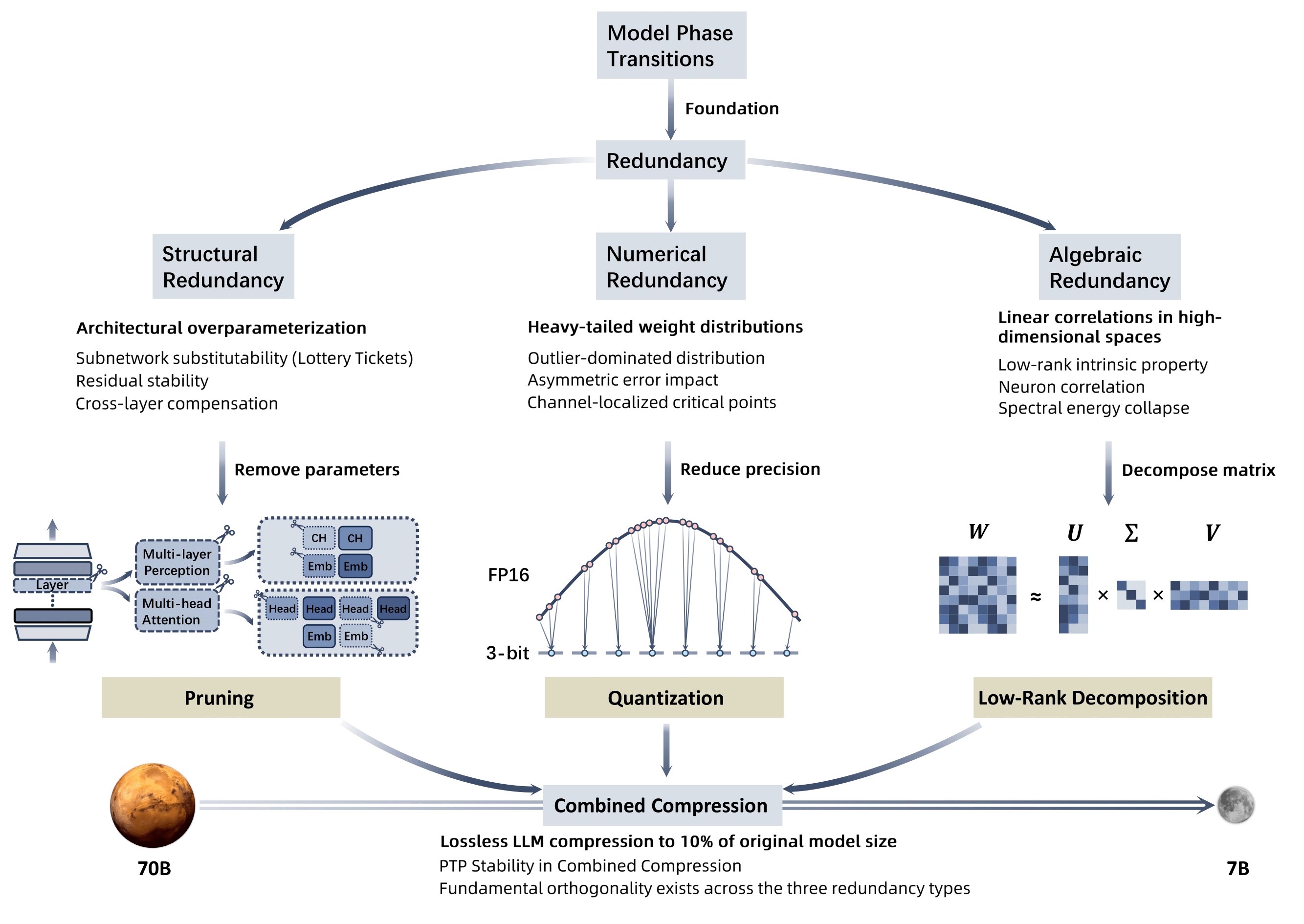
Large Language Models (LLMs) exhibit inherent redundancies that enable compression:
| Redundancy Type | Compression Technique | Description |
|---|---|---|
| Structural | Pruning | Architectural properties allow component removal (e.g., attention heads, layers) without functional loss |
| Numerical | Quantization | Heavy-tailed weight distributions permit precision reduction with minimal impact |
| Algebraic | Low-Rank Decomposition | Weight matrices exhibit low-rank properties enabling matrix factorization |
“The difference between a robustly-compressed model and a broken one is a single step past the PTP(Phase Transition Point).”
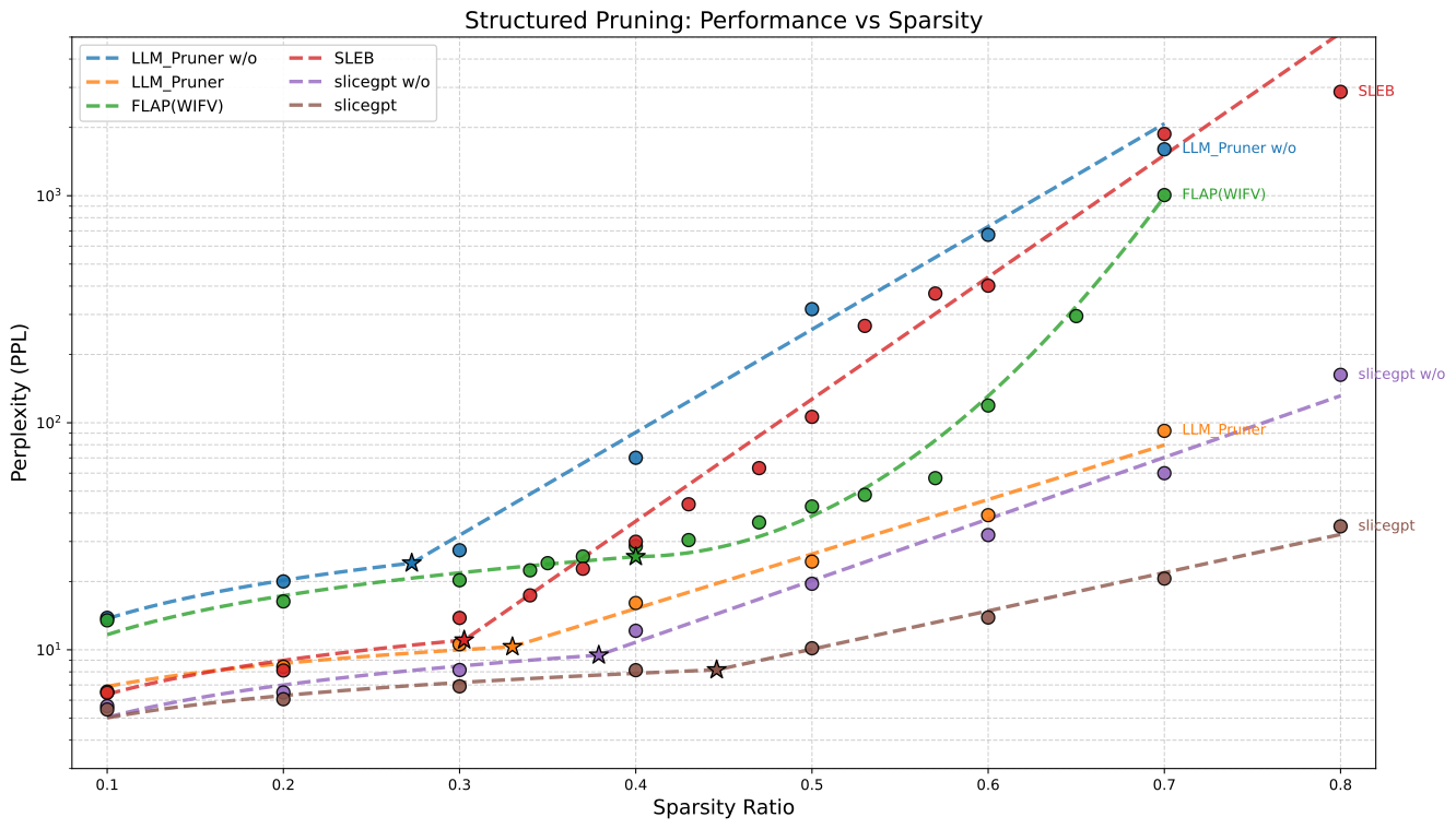
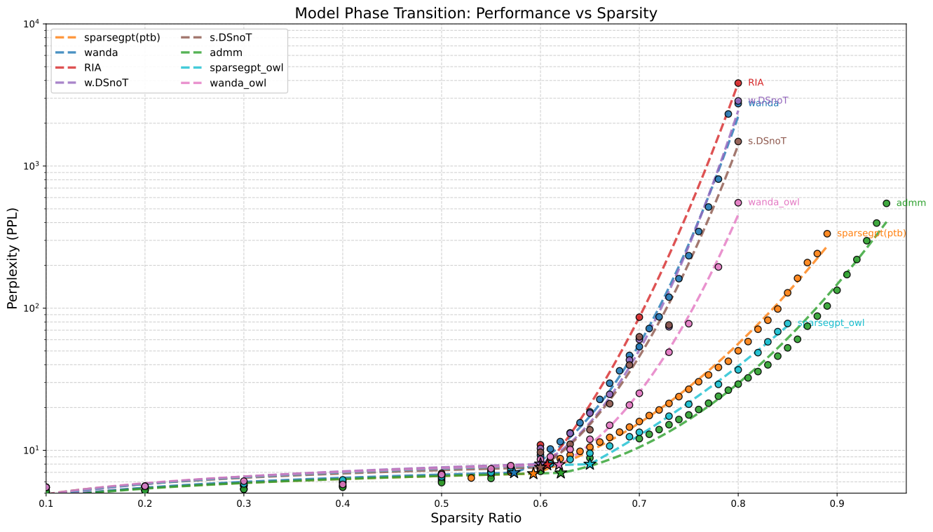
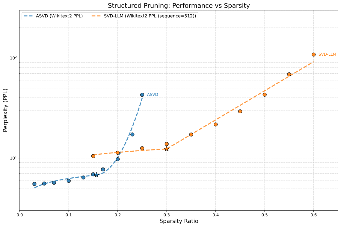
Fig. 3: This figure shows the perplexity (PPL) of several unstructured pruning methods across different sparsity ratios, including both experimental data and fitted curves. The stars indicate the turning points of the piecewise fitting curves, where the x-coordinate corresponds to the model’s phase transition point. The performance remains stable at lower sparsity ratios, but once the critical threshold is crossed, performance degradation becomes exponential.
Combined Pruning and Quantization
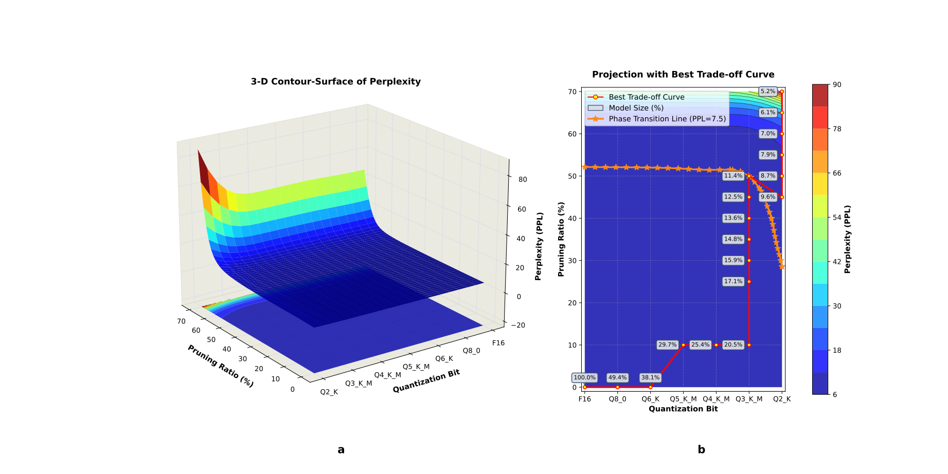
Fig. 6: Panel a presents the results of combining GGUF quantization and Wanda pruning on the LLaMA2-7b model. The 3D surface plot (Panel a) illustrates how perplexity (PPL) varies across different pruning ratios and quantization levels. The figure shows how the performance degrades with increasing compression, with the surface becoming steeper beyond a certain threshold. In Panel b, the 2D contour projection highlights the best trade-off curve between model size and perplexity. The red line marks the minimal PPL achieved at equivalent compression ratios, while the orange curve shows the phase transition line (PTL), indicating the point beyond which model performance rapidly deteriorates.
⭐️ Nature Machine Intelligence
Parameter-efficient fine-tuning of large-scale pre-trained language models
⭐️ Nature Communications
Efficient GPT-4V level multimodal large language model for deployment on edge devices
⭐️ SliceGPT (ICLR'24)
SliceGPT: Compress Large Language Models by Deleting Rows and Columns
Code
LLM-Pruner (NeurIPS'23)
LLM-Pruner: On the Structural Pruning of Large Language Models
Code
SLEB (ICML'24)
Streamlining LLMs through Redundancy Verification and Elimination of Transformer Blocks
Code
FLAP (AAAI'24)
Fluctuation-based Adaptive Structured Pruning for Large Language Models
Code
ShortGPT (arXiv)
Layers in Large Language Models are More Redundant Than You Expect
Sheared LLaMA (arXiv)
Accelerating Language Model Pre-training via Structured Pruning
Code
Shortened LLaMA (ICLR'24 Workshop)
Depth Pruning for LLMs with Comparison of Retraining Methods
SRAD (ICLR'25)
The Unreasonable Ineffectiveness of the Deeper Layers
LoRAPrune (ACL'24 Findings)
Structured Pruning Meets Low-Rank Parameter-Efficient Fine-Tuning
Code
⭐️ Wanda (ICML'23)
A Simple and Effective Pruning Approach for Large Language Models
Code
⭐️ SparseGPT (ICML'23)
Massive Language Models Can Be Accurately Pruned in One-Shot
Code
⭐️ ADMM (arXiv)
Fast and Effective Weight Update for Pruned Large Language Models
Code
RIA (ICLR'24)
Plug-and-Play: Efficient Post-training Pruning for LLMs
Code
DSnoT (ICLR'24)
Training-Free Fine-tuning for Sparse LLMs
Code
Flash-LLM (VLDB'24)
Cost-Effective and Efficient Inference with Unstructured Sparsity
Code
BESA (ICLR'24)
Blockwise Parameter-Efficient Sparsity Allocation
Code
GPTQ (ICLR'23)
Accurate Post-Training Quantization for Generative Pre-trained Transformers
Code
AWQ (MLSys'24)
Activation-aware Weight Quantization for LLMs
Code
SmoothQuant (ICML'23)
Accurate and Efficient Post-Training Quantization
Code
LLM.int8() (NeurIPS'22)
8-bit Matrix Multiplication for Transformers at Scale
Code
QLoRA (NeurIPS'23)
Efficient Finetuning of Quantized LLMs
Code
⭐️ GGUF
New quantized format for efficient LLM deployment
Code
ZeroQuant (NeurIPS'22)
Efficient and Affordable Post-Training Quantization for Large-Scale Transformers
Code
ASVD (arXiv)
Activation-aware SVD for Compressing Large Language Models
Code
⭐️ SVD-LLM (ICLR'25)
Truncation-aware SVD for Large Language Model Compression
Code
LoSparse (ICML'23)
Structured Compression based on Low-Rank and Sparse Approximation
Code
Lillama (NAACL'25)
One-shot Compression via Local Feature Distillation
Code
MoDeGPT (ICLR'25)
Modular Decomposition for Large Language Model Compression
Code
-1.png)
Fig. 7: This diagram illustrates structured pruning across model components, including neurons, attention heads, channels, sub-layers, and layers. The color intensity indicates the importance of each component: darker colors represent more critical parts, while lighter colors indicate less essential components, which are typically pruned first.
🔍 Cardinal sparsity thresholds for pruning
Pruning methods across different categories have specific cardinal sparsity thresholds that greatly affect their performance.
Structured pruning typically exhibits a critical sparsity threshold around 50%. Beyond this point, performance starts to degrade significantly, often leading to the collapse of the model. While it accelerates inference, the trade-off is often not worth it as the model’s accuracy is heavily impacted.
Unstructured pruning and semi-structured pruning methods can achieve much higher sparsity levels, with a threshold around 80%.
🏁 Horizontal comparisons across structured pruning, unstructured pruning, and semi-structured pruning
In a horizontal comparison, at similar compression rates, unstructured pruning consistently outperforms semi-structured pruning, which in turn, outperforms structured pruning.
🛠️ Problems with Existing Pruning Methods
Structured pruning's limitations: While pruning techniques have shown promise, they come with inherent limitations and trade-offs: While the main advantage of structured pruning lies in inference speedup, as highlighted in several recent papers, practical observations reveal that the trade-off between accuracy and speed is not always favorable. When sparsity exceeds 50%, the model generally collapses, providing less than a 2x speedup.
Semi-structured pruning's weaknesses: Recently, semi-structured pruning methods are often discussed alongside unstructured pruning, but they fail to outperform unstructured pruning and don't offer clear advantages of their own. In practice, while they can achieve moderate compression, they struggle to maintain model performance compared to unstructured pruning methods. Their overall lack of competitiveness at comparable compression rates raises questions about their utility.
Challenges in unstructured pruning: Unstructured pruning methods can achieve high compression rates (typically over 70%), but the performance trade-off is significant. Despite promising results in theory, practical applications face difficulties with acceleration. Many studies that use methods like Wanda and SparseGPT as baselines focus on extreme compression rates (>70%) for performance comparisons. However, these rates tend to cause catastrophic performance degradation, often referred to as "model hemorrhaging." In contrast, Wanda and SparseGPT perform better at lower sparsity levels, where other improved models fall short. Future research may need to shift focus towards performance at lower compression rates, possibly exploring combinations of pruning with quantization techniques to achieve better compression and faster inference without sacrificing too much accuracy.
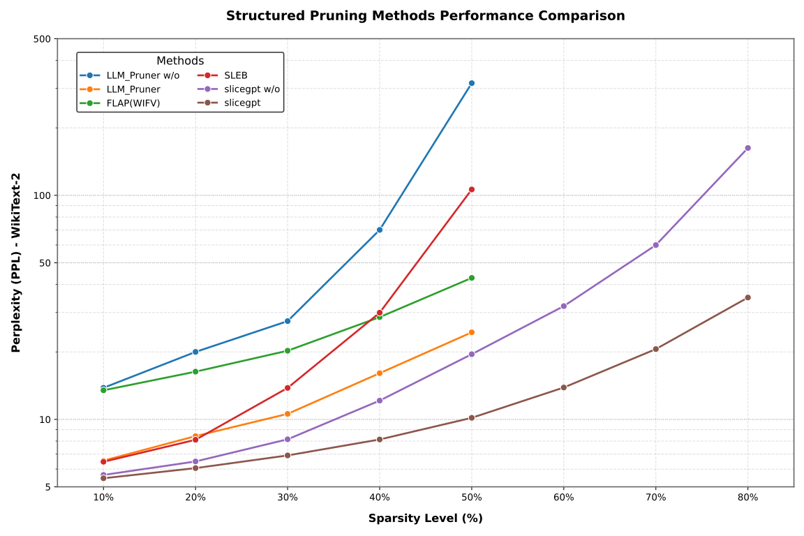
Fig. 8: Performance comparison of different structured pruning methods applied to LLaMA2-7b, based on the WikiText2-PPL (Perplexity) metric, across varying sparsity levels. The chart highlights the impact of pruning on model performance, with lower PPL values indicating better performance.
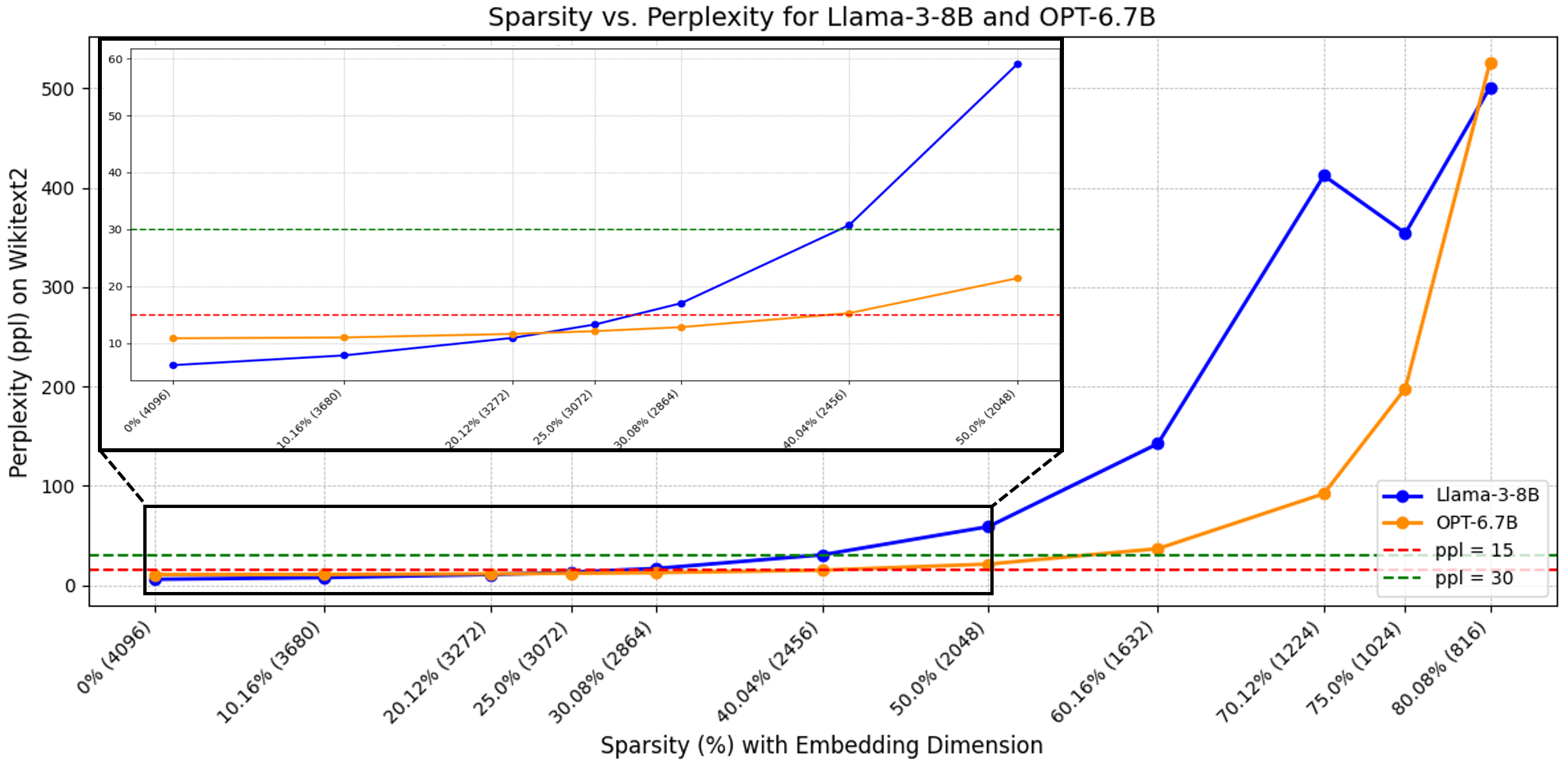
Fig. 9: Perplexity performance of LLaMA-3-8B and OPT-6.7B under different pruning ratios (Pruned by Slicegpt).
Table 1: WikiText2-PPL results for structured pruning (w/o: without finetuning)
| Method | 0.1 | 0.2 | 0.3 | 0.4 | 0.5 | 0.6 | 0.7 | 0.8 |
|---|---|---|---|---|---|---|---|---|
| LLM_Pruner w/o | 13.8316 | 20.0072 | 27.4537 | 70.1054 | 316.6549 | 672.9821 | 1601.8368 | - |
| LLM_Pruner | 6.5463 | 8.4221 | 10.5843 | 16.0763 | 24.4655 | 39.1722 | 92.1518 | - |
| FLAP(WIFV) | 13.4835 | 16.3325 | 20.2505 | 28.6018 | 42.7961 | 119.1558 | 1006.7369 | 2798.5380 |
| SLEB | 6.4700 | 8.1100 | 13.8200 | 29.9300 | 106.1900 | 401.5400 | 1870.92 | 2868.41 |
| slicegpt w/o | 5.6500 | 6.4900 | 8.1500 | 12.1300 | 19.5400 | 32.0300 | 59.9800 | 162.65 |
| slicegpt | 5.4610 | 6.0607 | 6.9047 | 8.1353 | 10.1622 | 13.8773 | 20.5934 | 34.9808 |
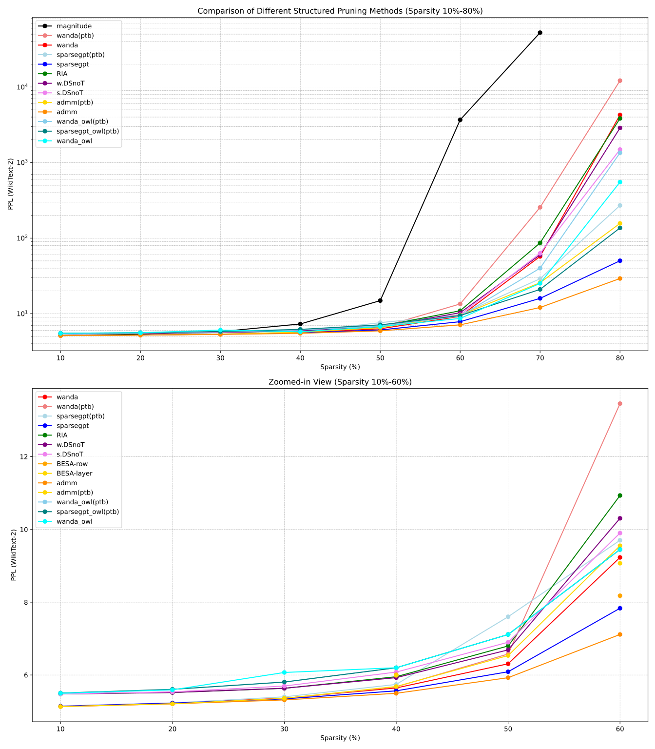
Fig. 10: WikiText2 perplexity (PPL) trends for various structured pruning methods across sparsity levels ranging from 10% to 80%. The upper part of the figure shows the overall trend across the full sparsity spectrum, while the lower part zooms in on the 10%--60% range to highlight differences among pruning methods at moderate compression levels. Methods with "(ptb)" suffix indicate usage of the PTB calibration dataset in ablation studies. The results show that while many pruning methods suffer significant performance drops at higher sparsity, approaches like Wanda, SparseGPT, and ADMM consistently preserve model quality under lower sparsity, suggesting greater robustness and practical viability. Note that the magnitude pruning curve is omitted from the lower subplot, as it consistently shows the worst degradation and dominates the y-axis range in zoomed-in views.
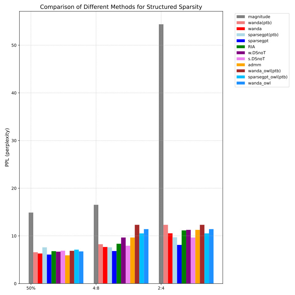
Fig. 11: Comparison of the performance of unstructured and structured pruning methods on WikiText2 PPL at 50% sparsity. The figure compares the perplexity (PPL) of various pruning methods for a model pruned to 50% sparsity. The methods include unstructured pruning (50%), and two types of structured pruning: 4:8 and 2:4, which indicate that 4 out of every 8 weights or 2 out of every 4 weights are pruned, respectively.
Table 2: WikiText2-PPL for different unstructured and semi-structured methods
| Method | 0.1 | 0.2 | 0.3 | 0.4 | 0.5 | 0.6 | 0.7 | 0.8 | 2:4(0.5) | 4:8(0.5) |
|---|---|---|---|---|---|---|---|---|---|---|
| Magnitude | 5.1737 | 5.3292 | 5.7920 | 7.3069 | 14.8954 | 3676.1436 | 52422.6016 | nan | 54.3870 | 16.5288 |
| Wanda | 5.1352 | 5.2269 | 5.3609 | 5.6434 | 6.3075 | 9.2307 | 57.2495 | 4262.4902 | 10.5414 | 7.6748 |
| SparseGPT | 5.1428 | 5.2277 | 5.3423 | 5.5635 | 6.0882 | 7.8341 | 15.9474 | 50.1593 | 8.1100 | 6.8299 |
| RIA | 5.4777 | 5.5181 | 5.6338 | 5.9517 | 6.7974 | 10.9329 | 86.4084 | 3832.7690 | 11.1520 | 8.3561 |
| w.DSnoT | 5.4789 | 5.5190 | 5.6344 | 5.9264 | 6.6898 | 10.3059 | 60.1499 | 2870.5852 | 11.2686 | 9.6594 |
| s.DSnoT | 5.4805 | 5.5347 | 5.6958 | 6.0794 | 6.8997 | 9.6878 | 62.8766 | 1487.4147 | 9.6594 | 7.9369 |
| ADMM | 5.1315 | 5.2076 | 5.3134 | 5.4959 | 5.9252 | 7.1137 | 12.0747 | 29.2164 | 7.5892 | 7.5892 |
| Wanda_owl | 5.4989 | 5.5901 | 6.0690 | 5.7550 | 6.7490 | 8.6492 | 25.1889 | 551.7274 | 11.4216 | - |
| BESA-row | - | - | - | - | 6.0057 | - | 8.1769 | - | - | - |
| BESA-layer | - | - | - | - | 5.9884 | - | 9.0709 | - | - | - |
Table 3: WikiText2-PPL for different unstructured and semi-structured methods calibrate on PTB dataset
| Method | 0.1 | 0.2 | 0.3 | 0.4 | 0.5 | 0.6 | 0.7 | 0.8 | 2:4(0.5) | 4:8(0.5) |
|---|---|---|---|---|---|---|---|---|---|---|
| Wanda | 5.1313 | 5.205 | 5.3455 | 5.6736 | 6.5758 | 13.4577 | 255.5912 | 12142.1484 | 12.5204 | 8.2569 |
| SparseGPT | 5.135 | 5.2305 | 5.3994 | 5.74 | 7.5999 | 9.7025 | 29.0151 | 270.8205 | 9.7025 | 7.5999 |
| Wanda_owl | 5.4885 | 5.5719 | 5.7487 | 6.0911 | 6.8722 | 9.3082 | 40.0371 | 1346.3525 | 12.3241 | - |
| SparseGPT_owl | 5.5043 | 5.6054 | 5.8055 | 6.1986 | 7.1123 | 9.4483 | 20.963 | 136.4502 | 10.5258 | - |
| ADMM | 5.1292 | 5.2079 | 5.3587 | 5.6827 | 6.5338 | 9.5521 | 25.6936 | 156.7145 | 10.0416 | 10.0416 |
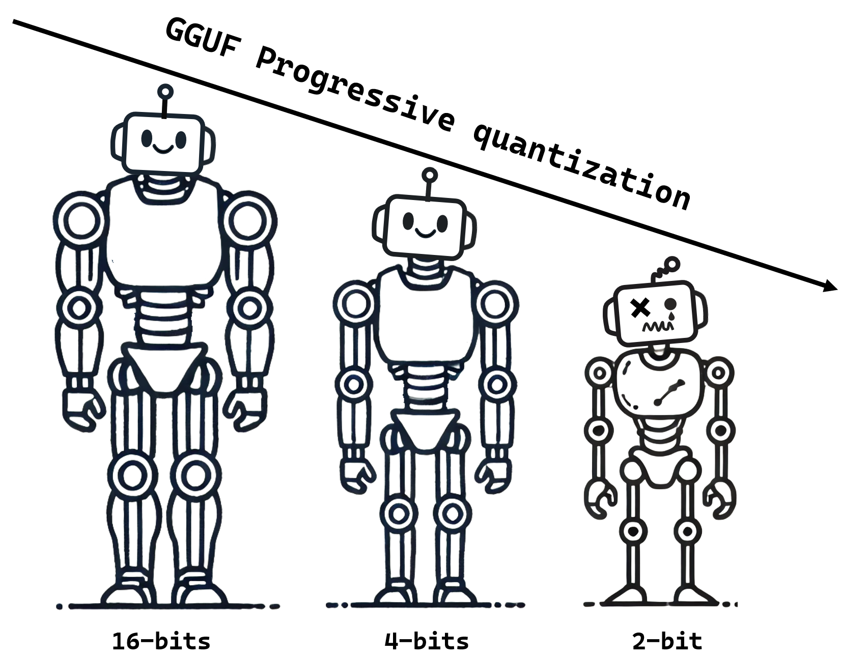
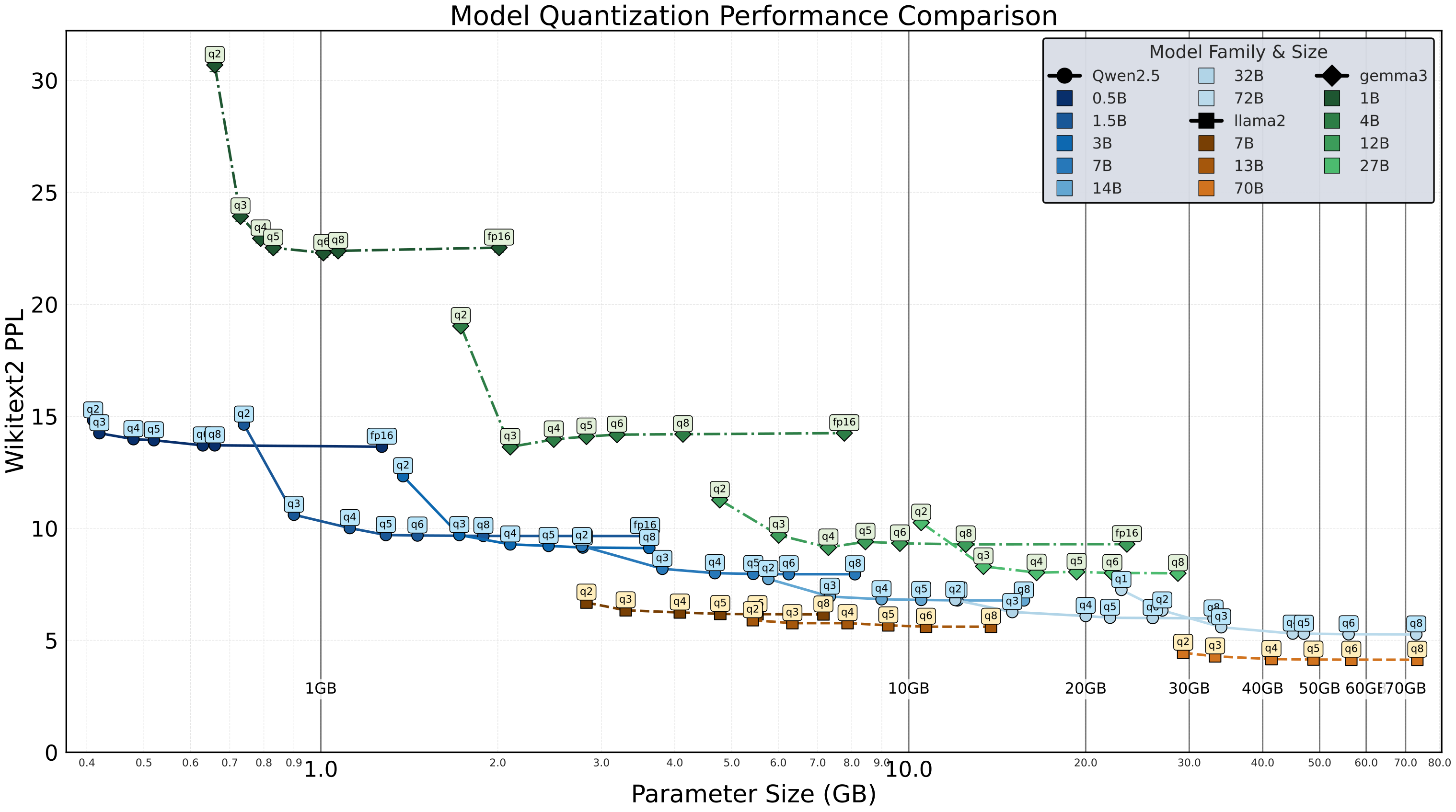
Fig. 12: GGUF progressive quantization with critical 3-bit threshold
-1.png)
Fig. 13: This figure compares symmetric (a) and asymmetric (b) quantization. In symmetric quantization, the intervals are evenly distributed around zero, while in asymmetric quantization, the intervals are non-symmetric, offering more flexibility for complex data distributions. The figure also shows the quantization and dequantization processes, with average loss values for both methods. Symmetric quantization typically results in higher average loss.
🔍 Lossless quantization thresholds
Quantization exhibits a "safe compression zone" (critical 3-bit threshold), beyond which performance degrades nonlinearly—yet larger models retain superior performance under low-bit settings compared to smaller "full-scale" counterparts at the same memory footprint.
🏁 Horizontal comparison of different models and different quantification methods
We conducted weight-only quantization experiments on base models of approximately 7B parameters using GPTQ with 8-bit and 4-bit precision. The models evaluated include LLaMA-3-8B, Mistral-7B, OPT-6.7B, Orca2-7B, and BLOOM-7.1B. The results indicate that most models exhibit stable performance after both 8-bit and 4-bit quantization.
We evaluate several widely used Post-Training Quantization (PTQ) methods on LLaMA2-7b, using the WikiText2 dataset and a maximum input length of 2K. The evaluation focuses on PPL (Perplexity) to assess the model's accuracy retention after quantization. The results show that most quantization methods maintain good accuracy, with a maximum precision loss of only 5% at 4-bit quantization.
📉 Progressive quantization curves at full model scale
To systematically evaluate the impact of model quantization on inference performance (PPL, inference speed, ARC-Easy, ARC-Challenge, and MMLU), we conducted comprehensive experiments on multiple models quantized via the GGUF framework. These experiments covered progressive quantization from 1-bit to 16-bit precision, focusing on well-performing yet moderately sized Qwen-2.5 model families (0.5B、1.5B,3B,7B,14B,32B,72B). Furthermore, given the remarkable performance recently exhibited by DeepSeek-R1, we also incorporated several DeepSeek-R1-distilled variants of LLaMA-3.1 and Qwen-2.5.
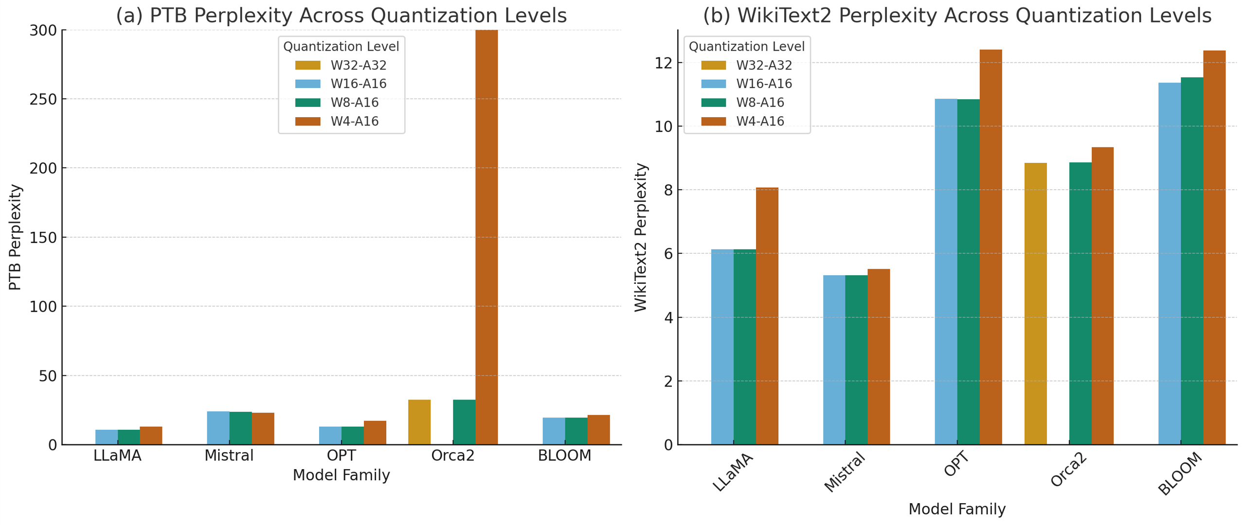
Fig. 14: Perplexity of 5 models across quantization levels. (a) PTB. (b) Wikitext2.
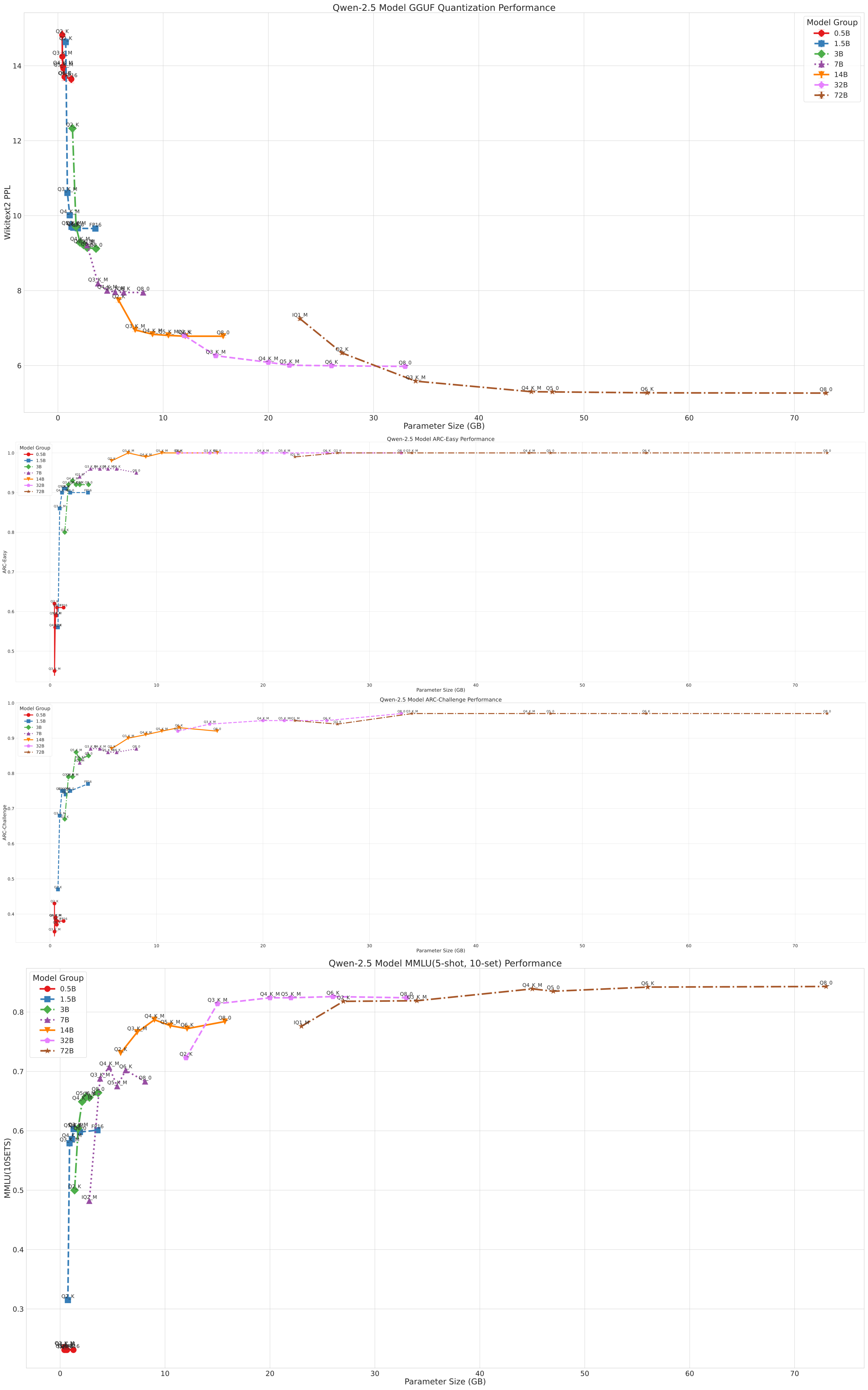
Fig. 15: The performance of the Qwen-2.5 model under various GGUF quantization schemes across multiple datasets and scales. This figure presents four subplots stacked vertically: (Top) WikiText2 perplexity (PPL), (Second) ARC-Easy accuracy, (Third) ARC-Challenge accuracy, (Bottom) MMLU accuracy. Results are shown across multiple model scales (0.5B, 1.5B, 3B, 7B, 14B, 32B, and 72B). These subplots demonstrate the performance trends of the Qwen-2.5 model under different quantization settings, helping to illustrate the impact of GGUF quantization on both perplexity and accuracy across a range of tasks and model sizes.
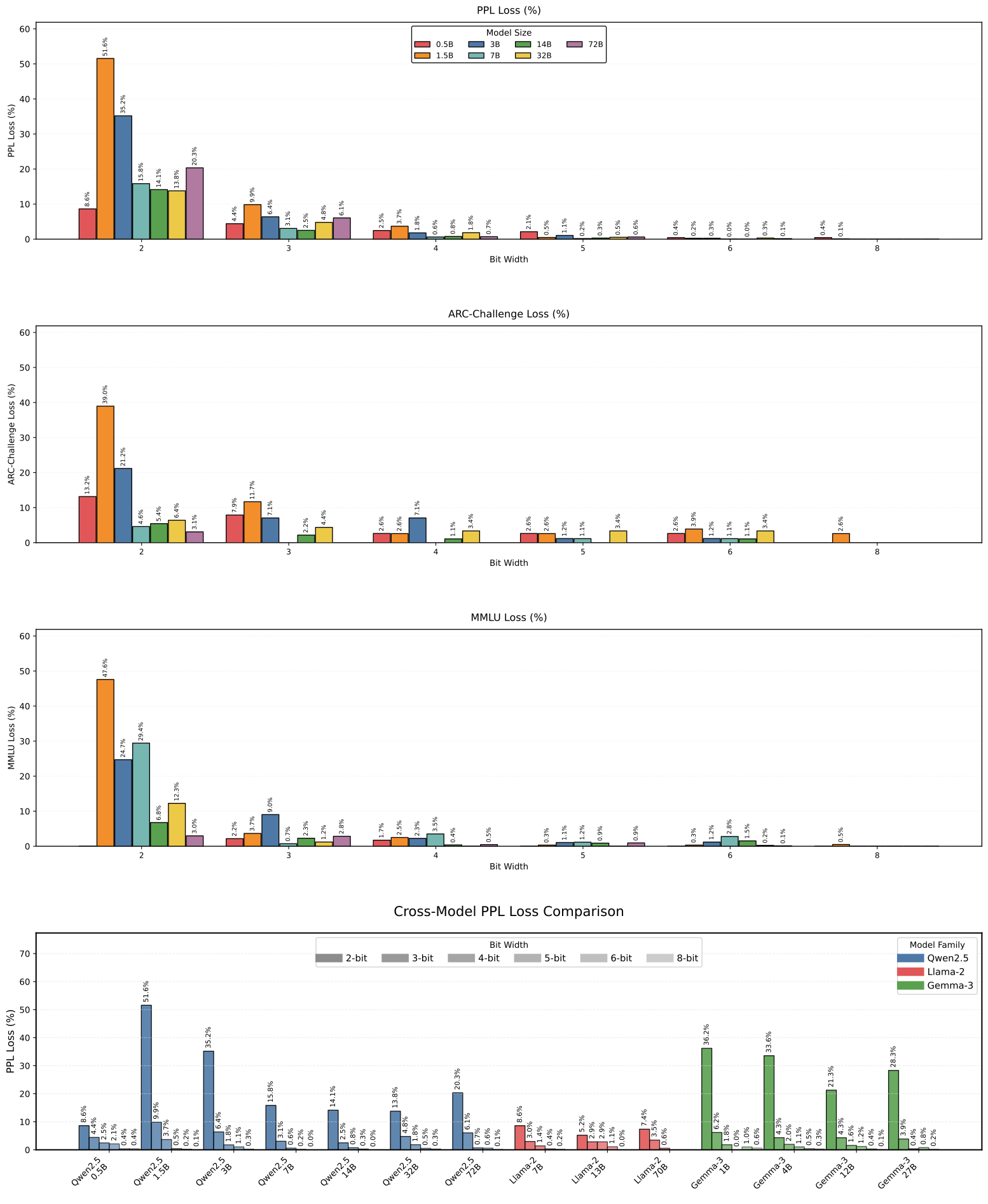
Fig. 16: Impact of 2-bit quantization on PPL, ARC-Challenge accuracy, and MMLU accuracy across model scales for various model families (Gemma-3, LLaMA-2, Owner-2.5).
Table 4:Wikitext2-PPL results for various quantization methods with different bit configurations(2K).
| Method | 2bits | 3bits | 4bits | 8bits |
|---|---|---|---|---|
| GPTQ | 1784.1625 | 7.5768 | 5.7459 | 5.4739 |
| AWQ | - | 6.2431 | 5.6009 | - |
| GGUF | 5.8619 | 5.5463 | 5.4549 | 5.3976 |
| QLoRA_NF4 | - | - | 5.6500 | - |
| QLoRA_FP4 | - | - | 5.7700 | - |
| LLM.int8() | - | - | - | 5.5000 |
| SmothQuant w8a8 | - | - | - | 5.5934 |
Table 5: Comprehensive evaluation of quantized models including perplexities (PPL), inference speed, parameter sizes, and downstream task performance (ARC-Easy, ARC-Challenge, and MMLU).
| Main Model | Indicator | 1-bit | 2-bit | 3-bit | 4-bit | 5-bit | 6-bit | 8-bit | 16-bit |
|---|---|---|---|---|---|---|---|---|---|
| Qwen2.5-0.5B | Quant Scheme | - | Q2_K | Q3_K_M | Q4_K_M | Q5_K_M | Q6_K | Q8_0 | FP16 |
| PPL | - | 14.82 ± 0.11 | 14.25 ± 0.11 | 13.98 ± 0.10 | 13.93 ± 0.10 | 13.70 ± 0.10 | 13.70 ± 0.10 | 13.64 ± 0.10 | |
| Tokens/s | - | 5593.60 | 5343.97 | 5370.62 | 5385.33 | 5427.74 | 5465.18 | 4266.22 | |
| Param(GB) | - | 0.41 | 0.42 | 0.48 | 0.52 | 0.63 | 0.66 | 1.27 | |
| ARC-C | - | 0.43 | 0.35 | 0.39 | 0.39 | 0.37 | 0.38 | 0.38 | |
| ARC-E | - | 0.62 | 0.45 | 0.56 | 0.59 | 0.59 | 0.61 | 0.61 | |
| MMLU | - | 0.23 | 0.24 | 0.24 | 0.23 | 0.23 | 0.23 | 0.23 | |
| Qwen2.5-1.5B | Quant Scheme | - | Q2_K | Q3_K_M | Q4_K_M | Q5_K_M | Q6_K | Q8_0 | FP16 |
| PPL | - | 14.63 ± 0.10 | 10.61 ± 0.07 | 10.01 ± 0.07 | 9.70 ± 0.07 | 9.68 ± 0.07 | 9.66 ± 0.07 | 9.66 ± 0.07 | |
| Tokens/s | - | 3814.78 | 3630.17 | 3843.72 | 3494.10 | 3543.53 | 3265.56 | 2133.91 | |
| Param(GB) | - | 0.74 | 0.90 | 1.12 | 1.29 | 1.46 | 1.89 | 3.56 | |
| ARC-C | - | 0.47 | 0.68 | 0.75 | 0.75 | 0.74 | 0.75 | 0.77 | |
| ARC-E | - | 0.56 | 0.86 | 0.90 | 0.91 | 0.91 | 0.90 | 0.90 | |
| MMLU | - | 0.32 | 0.58 | 0.59 | 0.60 | 0.60 | 0.60 | 0.60 | |
| Qwen2.5-3B | Quant Scheme | - | Q2_K | Q3_K_M | Q4_K_M | Q5_K_M | Q6_K | Q8_0 | FP16 |
| PPL | - | 12.33 ± 0.09 | 9.70 ± 0.07 | 9.28 ± 0.06 | 9.22 ± 0.06 | 9.14 ± 0.06 | 9.12 ± 0.06 | - | |
| Tokens/s | - | 2397.99 | 2166.52 | 2117.60 | 2005.48 | 1669.51 | 1427.80 | - | |
| Param(GB) | - | 1.38 | 1.72 | 2.10 | 2.44 | 2.79 | 3.62 | - | |
| ARC-C | - | 0.67 | 0.79 | 0.79 | 0.86 | 0.84 | 0.85 | - | |
| ARC-E | - | 0.80 | 0.92 | 0.93 | 0.92 | 0.92 | 0.92 | - | |
| MMLU | - | 0.50 | 0.60 | 0.65 | 0.66 | 0.66 | 0.66 | - | |
| Qwen2.5-7B | Quant Scheme | - | IQ2_M | Q3_K_M | Q4_K_M | Q5_K_M | Q6_K | Q8_0 | FP16 |
| PPL | - | 9.21 ± 0.06 | 8.19 ± 0.06 | 8.00 ± 0.05 | 7.96 ± 0.05 | 7.95 ± 0.05 | 7.95 ± 0.05 | - | |
| Tokens/s | - | 1439.49 | 952.80 | 1014.46 | 727.07 | 759.87 | 520.07 | - | |
| Param(GB) | - | 2.78 | 3.81 | 4.68 | 5.44 | 6.25 | 8.10 | - | |
| ARC-C | - | 0.83 | 0.87 | 0.87 | 0.86 | 0.86 | 0.87 | - | |
| ARC-E | - | 0.94 | 0.96 | 0.96 | 0.96 | 0.96 | 0.95 | - | |
| MMLU | - | 0.48 | 0.69 | 0.71 | 0.68 | 0.70 | 0.68 | - | |
| Qwen2.5-14B | Quant Scheme | - | Q2_K | Q3_K_M | Q4_K_M | Q5_K_M | Q6_K | Q8_0 | FP16 |
| PPL | - | 7.74 ± 0.05 | 6.95 ± 0.04 | 6.83 ± 0.04 | 6.80 ± 0.04 | 6.78 ± 0.04 | 6.78 ± 0.04 | - | |
| Tokens/s | - | 320.36 | 311.41 | 303.88 | 314.02 | 257.84 | 185.52 | - | |
| Param(GB) | - | 5.77 | 7.34 | 8.99 | 10.50 | 12.10 | 15.70 | - | |
| ARC-C | - | 0.87 | 0.90 | 0.91 | 0.92 | 0.93 | 0.92 | - | |
| ARC-E | - | 0.98 | 1.00 | 0.99 | 1.00 | 1.00 | 1.00 | - | |
| MMLU | - | 0.73 | 0.77 | 0.79 | 0.78 | 0.77 | 0.78 | - | |
| Qwen2.5-32B | Quant Scheme | - | Q2_K | Q3_K_M | Q4_K_M | Q5_K_M | Q6_K | Q8_0 | FP16 |
| PPL | - | 6.80 ± 0.04 | 6.26 ± 0.04 | 6.09 ± 0.04 | 6.01 ± 0.04 | 5.99 ± 0.04 | 5.98 ± 0.04 | - | |
| Tokens/s | - | 139.78 | 137.34 | 136.93 | 191.87 | 196.46 | 143.49 | - | |
| Param(GB) | - | 12.00 | 15.00 | 20.00 | 22.00 | 26.00 | 33.00 | - | |
| ARC-C | - | 0.92 | 0.94 | 0.95 | 0.95 | 0.95 | 0.98 | - | |
| ARC-E | - | 1.00 | 1.00 | 1.00 | 1.00 | 1.00 | 1.00 | - | |
| MMLU | - | 0.72 | 0.81 | 0.82 | 0.82 | 0.83 | 0.82 | - | |
| Qwen2.5-72B | Quant Scheme | IQ1_M | Q2_K | Q3_K_M | Q4_K_M | Q5_K_M | Q6_K | Q8_0 | - |
| PPL | 7.25 ± 0.05 | 6.34 ± 0.04 | 5.58 ± 0.03 | 5.30 ± 0.03 | 5.30 ± 0.03 | 5.27 ± 0.03 | 5.26 ± 0.03 | - | |
| Tokens/s | 96.60 | 100.13 | 83.56 | 62.33 | 95.96 | 108.05 | 177.27 | - | |
| Param(GB) | 23.70 | 29.80 | 37.70 | 47.40 | 47.00 | 56.00 | 73.00 | - | |
| ARC-C | 0.95 | 0.94 | 0.97 | 0.97 | 0.97 | 0.97 | 0.97 | - | |
| ARC-E | 0.99 | 1.00 | 1.00 | 1.00 | 1.00 | 1.00 | 1.00 | - | |
| MMLU | 0.78 | 0.82 | 0.82 | 0.84 | 0.83 | 0.84 | 0.84 | - | |
| DeepSeek-R1-Distill-Qwen-14B | Quant Scheme | - | Q2_K | Q3_K_M | Q4_K_M | Q5_K_M | Q6_K | Q8_0 | FP16 |
| PPL | - | 11.87 ± 0.10 | 9.81 ± 0.08 | 9.45 ± 0.07 | 9.39 ± 0.07 | 9.38 ± 0.07 | 9.39 ± 0.07 | - | |
| Tokens/s | - | 497.57 | 405.06 | 420.73 | 403.24 | 263.45 | 257.80 | - | |
| Param(GB) | - | 5.77 | 7.34 | 8.99 | 10.51 | 12.12 | 15.70 | - | |
| DeepSeek-R1-Distill-Llama-8B | Quant Scheme | - | Q2_K | Q3_K_M | Q4_K_M | Q5_K_M | Q6_K | Q8_0 | FP16 |
| PPL | - | 17.86 ± 0.15 | 13.96 ± 0.11 | 13.12 ± 0.11 | 12.94 ± 0.11 | 12.86 ± 0.10 | 12.84 ± 0.10 | 12.85 ± 0.10 | |
| Tokens/s | - | 1105.20 | 799.52 | 914.69 | 1015.46 | 942.53 | 809.24 | 299.60 | |
| Param(GB) | - | 3.18 | 4.02 | 4.92 | 5.73 | 6.60 | 8.54 | 16.10 | |
| Llama-3.1-8B | Quant Scheme | - | Q2_K | Q3_K_M | Q4_K_M | Q5_K_M | Q6_K | Q8_0 | FP16 |
| PPL | - | 9.02 ± 0.06 | 7.81 ± 0.05 | 7.53 ± 0.05 | 7.45 ± 0.05 | 7.43 ± 0.05 | 7.41 ± 0.05 | - | |
| Tokens/s | - | 817.69 | 1031.46 | 919.29 | 561.81 | 570.54 | 435.94 | - | |
| Param(GB) | - | 2.95 | 4.02 | 4.92 | 5.73 | 6.60 | 8.54 | - |
Table 6: WikiText2-PPL and parameter sizes for LLaMA-2 and Gemma-3 model families.
| Main Model | Quant Scheme | PPL | Param(GB) |
|---|---|---|---|
| LLaMA-2-70B | Q5_K_M | 4.14 ± 0.02 | 48.80 |
| Q4_K_M | 4.16 ± 0.02 | 41.40 | |
| Q3_K_M | 4.28 ± 0.02 | 33.20 | |
| Q2_K_M | 4.44 ± 0.02 | 29.30 | |
| LLaMA-2-13B | Q8_K_0 | 5.61 ± 0.03 | 13.80 |
| Q6_K | 5.61 ± 0.03 | 10.70 | |
| Q5_K_M | 5.67 ± 0.03 | 9.23 | |
| Q4_K_M | 5.77 ± 0.03 | 7.87 | |
| Q3_K_M | 5.77 ± 0.03 | 6.34 | |
| Q2_K_M | 5.90 ± 0.03 | 5.43 | |
| LLaMA-2-7B | Q8_K_0 | 6.16 ± 0.03 | 7.16 |
| Q6_K | 6.17 ± 0.03 | 5.53 | |
| Q5_K_M | 6.18 ± 0.03 | 4.78 | |
| Q4_K_M | 6.24 ± 0.03 | 4.08 | |
| Q3_K_M | 6.34 ± 0.04 | 3.30 | |
| Q2_K | 6.69 ± 0.04 | 2.83 | |
| Gemma-3-27B-IT | Q8_0 | 7.99 ± 0.06 | 28.70 |
| Q6_K | 8.01 ± 0.06 | 22.20 | |
| Q5_K_M | 8.05 ± 0.06 | 19.30 | |
| Q4_K_M | 8.02 ± 0.06 | 16.50 | |
| Q3_K_M | 8.30 ± 0.06 | 13.40 | |
| Q2_K | 10.25 ± 0.08 | 10.50 | |
| Gemma-3-12B-IT | FP16 | 9.29 ± 0.07 | 23.50 |
| Q8_0 | 9.28 ± 0.07 | 12.50 | |
| Q6_K | 9.33 ± 0.07 | 9.66 | |
| Q5_K_M | 9.40 ± 0.07 | 8.44 | |
| Q4_K_M | 9.15 ± 0.07 | 7.30 | |
| Q3_K_M | 9.69 ± 0.08 | 6.01 | |
| Q2_K | 11.27 ± 0.09 | 4.77 | |
| Gemma-3-4B-IT | FP16 | 14.25 ± 0.13 | 7.77 |
| Q8_0 | 14.20 ± 0.13 | 4.13 | |
| Q6_K | 14.18 ± 0.13 | 3.19 | |
| Q5_K_M | 14.10 ± 0.13 | 2.83 | |
| Q4_K_M | 13.97 ± 0.13 | 2.49 | |
| Q3_K_M | 13.63 ± 0.12 | 2.10 | |
| Q2_K | 19.03 ± 0.17 | 1.73 | |
| Gemma-3-1B-IT | FP16 | 22.53 ± 0.20 | 2.01 |
| Q8_0 | 22.39 ± 0.20 | 1.07 | |
| Q6_K | 22.30 ± 0.20 | 1.01 | |
| Q5_K_M | 22.53 ± 0.20 | 0.83 | |
| Q4_K_M | 22.94 ± 0.21 | 0.79 | |
| Q3_K_M | 23.93 ± 0.22 | 0.73 | |
| Q2_K | 30.69 ± 0.29 | 0.66 |
🔍 Critical compression thresholds
In the domain of large language models, low-rank decomposition methods inherently offer limited compression ratios, as weight matrices in contemporary LLMs often exhibit near-full-rank characteristics. ASVD exhibits a phase transition at 17% rank reduction; beyond this point, PPL degrades exponentially. SVD-LLM’s phase transition occurs at 30%, indicating slightly higher compression tolerance but steeper collapse thereafter.
Table 7: Low-Rank Decomposition Results
| ASVD Sparsity | 0% | 3% | 5% | 7% | 10% | 13% | 15% | 17% | 20% | 23% | 25% | 27% |
|---|---|---|---|---|---|---|---|---|---|---|---|---|
| WikiText2 PPL | 5.45 | 5.52 | 5.56 | 5.67 | 5.92 | 6.40 | 6.89 | 7.70 | 9.73 | 17.20 | 42.83 | 259.05 |
| PTB PPL | 20.90 | 22.56 | 23.58 | 26.19 | 33.11 | 49.30 | 65.88 | 93.67 | 144.23 | 230.25 | 550.54 | 1248.51 |
| SVD-LLM Sparsity | 15% | 20% | 25% | 30% | 35% | 40% | 45% | 50% | 55% | 60% |
|---|---|---|---|---|---|---|---|---|---|---|
| WikiText2 PPL (seq=512) | 10.47 | 11.31 | 12.54 | 14.33 | 17.17 | 21.67 | 29.26 | 42.99 | 68.54 | 108.13 |
This section examines synergistic effects of combined compression strategies. We employ LLaMA2-7B as the unified testbed across all experiments.
| Pruning Ratio (%) | FP16 (Wikitext2 / PTB) | RTN_INT8 (Wikitext2 / PTB) | RTN_INT6 (Wikitext2 / PTB) |
|---|---|---|---|
| 0 | 5.450 / 20.898 | 5.452 / 20.906 | 5.501 / 21.060 |
| 3 | 5.519 / 22.564 | 5.520 / 22.529 | 5.570 / 23.214 |
| 5 | 5.564 / 23.584 | 5.566 / 23.708 | 5.621 / 24.770 |
| 7 | 5.672 / 26.192 | 5.674 / 26.601 | 5.732 / 31.670 |
| 10 | 5.924 / 33.113 | 5.910 / 31.539 | 5.987 / 36.262 |
| 13 | 6.402 / 49.298 | 6.406 / 49.359 | 6.513 / 62.393 |
| 15 | 6.886 / 65.879 | 6.901 / 63.252 | 7.026 / 117.559 |
| 17 | 7.699 / 93.670 | 7.710 / 89.613 | 7.942 / 132.180 |
| 20 | 9.735 / 144.226 | 9.804 / 141.177 | 10.283 / 158.376 |
| 23 | 17.203 / 230.252 | 17.456 / 232.298 | 18.936 / 277.449 |
| 25 | 42.828 / 550.543 | 43.161 / 558.946 | 47.348 / 696.396 |
| 27 | 259.052 / 1248.507 | 255.688 / 1256.895 | 231.828 / 1262.418 |
| Pruning Ratio | Budget / PPL (FP16) | Budget / PPL (8-bit) | Budget / PPL (4-bit) | Budget / PPL (3-bit) |
|---|---|---|---|---|
| 10% | 90.00% / 5.1429 | 44.70% / 5.1452 | 26.00% / 5.4323 | 20.50% / 11.1320 |
| 20% | 80.00% / 5.2286 | 39.70% / 5.2280 | 23.10% / 5.4564 | 18.20% / 9.8942 |
| 30% | 70.00% / 5.3413 | 34.70% / 5.3437 | 20.20% / 5.5484 | 16.00% / 10.5496 |
| 40% | 60.00% / 5.5667 | 29.80% / 5.5688 | 17.30% / 5.8095 | 13.70% / 10.9149 |
| 50% | 50.00% / 6.0806 | 24.80% / 6.0904 | 14.40% / 6.5168 | 11.40% / 9.0980 |
| 55% | 45.00% / 6.6764 | 22.30% / 6.6798 | 13.00% / 7.0401 | 10.30% / 14.3934 |
| 60% | 40.00% / 7.8854 | 19.90% / 7.8473 | 11.60% / 8.4310 | 9.10% / 13.2198 |
| 65% | 35.00% / 10.5544 | 17.40% / 10.5977 | 10.10% / 12.2171 | 8.00% / 22.0760 |
| 70% | 30.00% / 15.9313 | 14.90% / 15.7857 | 8.60% / 19.4003 | 6.80% / 33.2873 |
| 75% | 25.00% / 26.6704 | 12.40% / 26.9113 | 7.20% / 31.8896 | 5.70% / 44.8067 |
| 80% | 20.00% / 49.1943 | 10.00% / 50.8971 | 5.70% / 58.9694 | 4.50% / 109.4458 |
| Pruning Ratio | FP16 (Dense) | Q8_0 (size) | Q6_K (size) | Q5_K_M (size) | Q4_K_M (size) | Q3_K_M (size) | Q2_K (size) |
|---|---|---|---|---|---|---|---|
| 0% | 6.1565 (100%) | 6.1557 (49.4%) | 6.1682 (38.15%) | 6.1789 (38.15%) | 6.2427 (32.96%) | 6.3397 (22.74%) | 6.6850 (17.48%) |
| 10% | 6.1951 (90%) | 6.1948 (44.46%) | 6.2074 (34.34%) | 6.2099 (29.66%) | 6.2730 (25.35%) | 6.3795 (20.47%) | 7.1657 (15.73%) |
| 15% | 6.2488 (85%) | 6.2501 (41.99%) | 6.2614 (32.42%) | 6.2659 (28.02%) | 6.3209 (23.93%) | 6.4460 (19.33%) | 7.2316 (14.86%) |
| 20% | 6.3090 (80%) | 6.3090 (39.52%) | 6.3210 (30.52%) | 6.3304 (30.52%) | 6.3695 (22.52%) | 6.5112 (18.19%) | 7.3108 (13.98%) |
| 25% | 6.3549 (75%) | 6.3558 (37.05%) | 6.3710 (28.61%) | 6.3751 (24.72%) | 6.4141 (21.11%) | 6.5485 (17.06%) | 7.4179 (13.11%) |
| 30% | 6.4436 (70%) | 6.4448 (34.50%) | 6.4562 (26.70%) | 6.4675 (23.10%) | 6.5000 (19.70%) | 6.6262 (15.90%) | 7.5505 (12.20%) |
| 35% | 6.5539 (65%) | 6.5549 (32.11%) | 6.5662 (24.80%) | 6.5760 (21.42%) | 6.6179 (18.30%) | 6.7450 (14.78%) | 7.8072 (11.36%) |
| 40% | 6.7076 (60%) | 6.7097 (29.50%) | 6.7212 (22.90%) | 6.7374 (19.80%) | 6.7779 (16.90%) | 6.8962 (13.60%) | 8.0539 (10.50%) |
| 45% | 6.8927 (45%) | 6.8952 (27.17%) | 6.9050 (20.98%) | 6.9222 (18.13%) | 6.9593 (15.48%) | 7.0964 (12.51%) | 8.5137 (9.61%) |
| 50% | 7.2500 (50%) | 7.2608 (24.60%) | 7.2683 (19.00%) | 7.2954 (16.50%) | 7.3325 (14.10%) | 7.4961 (11.40%) | 9.3014 (8.70%) |
| 55% | 7.9666 (55%) | 7.9691 (22.23%) | 7.9810 (17.17%) | 8.0378 (14.83%) | 8.0717 (12.67%) | 8.3129 (10.23%) | 10.8619 (7.87%) |
| 60% | 9.8966 (40%) | 9.8964 (19.70%) | 9.9680 (15.20%) | 10.0972 (13.20%) | 10.1072 (11.30%) | 10.5264 (9.10%) | 15.1769 (7.00%) |
| 65% | 18.2312 (35%) | 18.2539 (17.29%) | 18.6984 (13.35%) | 18.9243 (11.54%) | 19.0064 (9.85%) | 20.3420 (7.96%) | 31.1628 (6.12%) |
| 70% | 47.7228 (30%) | 47.8818 (14.82%) | 48.6469 (11.45%) | 48.5954 (9.89%) | 48.3925 (8.45%) | 53.9657 (6.82%) | 86.6058 (5.24%) |
Note: Each cell shows PPL (top) and relative model size (bottom) compared to the original FP16 model at 0% pruning.
🏁 We compare various model compression methods, including both pruning and quantization techniques, under a 50% sparsity setting. The LLaMA2-7b model was tested on the WikiText2 dataset using Perplexity (PPL) as the performance metric. The results indicate that quantization outperforms pruning methods in terms of accuracy retention, with the ranking of performance being: Quantization > Unstructured Pruning > Semi-structured Pruning > Structured Pruning Low-Rank Decomposition.
%20on%20a%20log%20scale%20across%20two%20sparsity%20configurations..svg)
Fig. 17: Comparative analysis of model compression approaches evaluating perplexity (PPL) on a log scale across two sparsity configurations. Top: 50% sparsity performance across four strategy types - quantization (PPL 5.4-5.8), unstructured pruning (PPL 5.9-14.9), semi-structured pruning (PPL 6.8-16.5), structured pruning (PPL 10.2-316.7), and low-rank decomposition (PPL 43.0-nan). Bottom: 4-bit quantization methods (PPL 5.5-5.8) versus 70% unstructured pruning techniques (PPL 12.1-52.4k). Lower values indicate better language modeling capability retention, demonstrating quantization's stability versus pruning's extreme PPL variance at high sparsity.
Below are the primary models used in this project:
If you find this work useful, please consider citing:
@article{Ma2026PhaseTI,
  title={Phase transitions in large language model compression},
  author={Ziyang Ma and Zuchao Li and Lefei Zhang and Gui-Song Xia and Bo Du and Liangpei Zhang and Dacheng Tao},
  journal={npj Artificial Intelligence},
  year={2026},
  volume={2},
  url={https://api.semanticscholar.org/CorpusID:285307574}
}
43 followers · starred Jul 2025
Navigating Model Phase Transitions to Enable Extreme Lossless Compression: A Perspective
76
60 commits
updated Feb 9, 2026
Navigating Model Phase Transitions to Enable Extreme Lossless Compression
[2026] Our work Model Phase Transitions in Large Language Model Compression has been accepted as a Perspective by
npj | Artificial Intelligence (Nature Portfolio).
This paper provides a unifying theoretical and empirical framework for understanding phase transitions in model compression, revealing how orthogonal redundancy sources jointly determine the limits of lossless compression in large language models.
📄 Paper: npj | Artificial Intelligence (Nature)
🔗 https://www.nature.com/articles/s44387-026-00072-8
The increasing size and complexity of large language models (LLMs) present significant computational and memory challenges. To address these challenges, model compression techniques have been developed to reduce the resource demands of LLMs. However, compression techniques can exhibit Model Phase Transitions (MPT), where the model's performance remains stable until a critical threshold is reached, after which the performance degrades sharply. The key to achieving effective compression lies in understanding model redundancy, which provides buffers that allow for compression until this phase transition point is reached.
In our work, we introduce the concept of Model Phase Transition to fundamentally characterize performance degradation and lossless compression limits in large language models. Across more than thirty pruning, quantization, and low-rank decomposition techniques, we fit performance trajectories with a novel piecewise power-law–exponential curve that pinpoints each technique’s phase-transition point (PTP): structured pruning fails at 30–45% sparsity, unstructured pruning at 55–65%, low-rank decomposition at 17–30%, and quantization below 3-bit precision. Crucially, these redundancy sources are orthogonal: by staying within the joint safe region defined by their PTPs, we raise the prior single-dimension bottleneck, enabling lossless compression to 10% of original model size.
If you find any errors or have suggestions, feel free to reach out: [email protected]
Large Language Models (LLMs) exhibit inherent redundancies that enable compression:
| Redundancy Type | Compression Technique | Description |
|---|---|---|
| Structural | Pruning | Architectural properties allow component removal (e.g., attention heads, layers) without functional loss |
| Numerical | Quantization | Heavy-tailed weight distributions permit precision reduction with minimal impact |
| Algebraic | Low-Rank Decomposition | Weight matrices exhibit low-rank properties enabling matrix factorization |
“The difference between a robustly-compressed model and a broken one is a single step past the PTP(Phase Transition Point).”
Fig. 3: This figure shows the perplexity (PPL) of several unstructured pruning methods across different sparsity ratios, including both experimental data and fitted curves. The stars indicate the turning points of the piecewise fitting curves, where the x-coordinate corresponds to the model’s phase transition point. The performance remains stable at lower sparsity ratios, but once the critical threshold is crossed, performance degradation becomes exponential.
Combined Pruning and Quantization
Fig. 6: Panel a presents the results of combining GGUF quantization and Wanda pruning on the LLaMA2-7b model. The 3D surface plot (Panel a) illustrates how perplexity (PPL) varies across different pruning ratios and quantization levels. The figure shows how the performance degrades with increasing compression, with the surface becoming steeper beyond a certain threshold. In Panel b, the 2D contour projection highlights the best trade-off curve between model size and perplexity. The red line marks the minimal PPL achieved at equivalent compression ratios, while the orange curve shows the phase transition line (PTL), indicating the point beyond which model performance rapidly deteriorates.
⭐️ Nature Machine Intelligence
Parameter-efficient fine-tuning of large-scale pre-trained language models
⭐️ Nature Communications
Efficient GPT-4V level multimodal large language model for deployment on edge devices
⭐️ SliceGPT (ICLR'24)
SliceGPT: Compress Large Language Models by Deleting Rows and Columns
Code
LLM-Pruner (NeurIPS'23)
LLM-Pruner: On the Structural Pruning of Large Language Models
Code
SLEB (ICML'24)
Streamlining LLMs through Redundancy Verification and Elimination of Transformer Blocks
Code
FLAP (AAAI'24)
Fluctuation-based Adaptive Structured Pruning for Large Language Models
Code
ShortGPT (arXiv)
Layers in Large Language Models are More Redundant Than You Expect
Sheared LLaMA (arXiv)
Accelerating Language Model Pre-training via Structured Pruning
Code
Shortened LLaMA (ICLR'24 Workshop)
Depth Pruning for LLMs with Comparison of Retraining Methods
SRAD (ICLR'25)
The Unreasonable Ineffectiveness of the Deeper Layers
LoRAPrune (ACL'24 Findings)
Structured Pruning Meets Low-Rank Parameter-Efficient Fine-Tuning
Code
⭐️ Wanda (ICML'23)
A Simple and Effective Pruning Approach for Large Language Models
Code
⭐️ SparseGPT (ICML'23)
Massive Language Models Can Be Accurately Pruned in One-Shot
Code
⭐️ ADMM (arXiv)
Fast and Effective Weight Update for Pruned Large Language Models
Code
RIA (ICLR'24)
Plug-and-Play: Efficient Post-training Pruning for LLMs
Code
DSnoT (ICLR'24)
Training-Free Fine-tuning for Sparse LLMs
Code
Flash-LLM (VLDB'24)
Cost-Effective and Efficient Inference with Unstructured Sparsity
Code
BESA (ICLR'24)
Blockwise Parameter-Efficient Sparsity Allocation
Code
GPTQ (ICLR'23)
Accurate Post-Training Quantization for Generative Pre-trained Transformers
Code
AWQ (MLSys'24)
Activation-aware Weight Quantization for LLMs
Code
SmoothQuant (ICML'23)
Accurate and Efficient Post-Training Quantization
Code
LLM.int8() (NeurIPS'22)
8-bit Matrix Multiplication for Transformers at Scale
Code
QLoRA (NeurIPS'23)
Efficient Finetuning of Quantized LLMs
Code
⭐️ GGUF
New quantized format for efficient LLM deployment
Code
ZeroQuant (NeurIPS'22)
Efficient and Affordable Post-Training Quantization for Large-Scale Transformers
Code
ASVD (arXiv)
Activation-aware SVD for Compressing Large Language Models
Code
⭐️ SVD-LLM (ICLR'25)
Truncation-aware SVD for Large Language Model Compression
Code
LoSparse (ICML'23)
Structured Compression based on Low-Rank and Sparse Approximation
Code
Lillama (NAACL'25)
One-shot Compression via Local Feature Distillation
Code
MoDeGPT (ICLR'25)
Modular Decomposition for Large Language Model Compression
Code
Fig. 7: This diagram illustrates structured pruning across model components, including neurons, attention heads, channels, sub-layers, and layers. The color intensity indicates the importance of each component: darker colors represent more critical parts, while lighter colors indicate less essential components, which are typically pruned first.
🔍 Cardinal sparsity thresholds for pruning
Pruning methods across different categories have specific cardinal sparsity thresholds that greatly affect their performance.
Structured pruning typically exhibits a critical sparsity threshold around 50%. Beyond this point, performance starts to degrade significantly, often leading to the collapse of the model. While it accelerates inference, the trade-off is often not worth it as the model’s accuracy is heavily impacted.
Unstructured pruning and semi-structured pruning methods can achieve much higher sparsity levels, with a threshold around 80%.
🏁 Horizontal comparisons across structured pruning, unstructured pruning, and semi-structured pruning
In a horizontal comparison, at similar compression rates, unstructured pruning consistently outperforms semi-structured pruning, which in turn, outperforms structured pruning.
🛠️ Problems with Existing Pruning Methods
Structured pruning's limitations: While pruning techniques have shown promise, they come with inherent limitations and trade-offs: While the main advantage of structured pruning lies in inference speedup, as highlighted in several recent papers, practical observations reveal that the trade-off between accuracy and speed is not always favorable. When sparsity exceeds 50%, the model generally collapses, providing less than a 2x speedup.
Semi-structured pruning's weaknesses: Recently, semi-structured pruning methods are often discussed alongside unstructured pruning, but they fail to outperform unstructured pruning and don't offer clear advantages of their own. In practice, while they can achieve moderate compression, they struggle to maintain model performance compared to unstructured pruning methods. Their overall lack of competitiveness at comparable compression rates raises questions about their utility.
Challenges in unstructured pruning: Unstructured pruning methods can achieve high compression rates (typically over 70%), but the performance trade-off is significant. Despite promising results in theory, practical applications face difficulties with acceleration. Many studies that use methods like Wanda and SparseGPT as baselines focus on extreme compression rates (>70%) for performance comparisons. However, these rates tend to cause catastrophic performance degradation, often referred to as "model hemorrhaging." In contrast, Wanda and SparseGPT perform better at lower sparsity levels, where other improved models fall short. Future research may need to shift focus towards performance at lower compression rates, possibly exploring combinations of pruning with quantization techniques to achieve better compression and faster inference without sacrificing too much accuracy.
Fig. 8: Performance comparison of different structured pruning methods applied to LLaMA2-7b, based on the WikiText2-PPL (Perplexity) metric, across varying sparsity levels. The chart highlights the impact of pruning on model performance, with lower PPL values indicating better performance.
Fig. 9: Perplexity performance of LLaMA-3-8B and OPT-6.7B under different pruning ratios (Pruned by Slicegpt).
Table 1: WikiText2-PPL results for structured pruning (w/o: without finetuning)
| Method | 0.1 | 0.2 | 0.3 | 0.4 | 0.5 | 0.6 | 0.7 | 0.8 |
|---|---|---|---|---|---|---|---|---|
| LLM_Pruner w/o | 13.8316 | 20.0072 | 27.4537 | 70.1054 | 316.6549 | 672.9821 | 1601.8368 | - |
| LLM_Pruner | 6.5463 | 8.4221 | 10.5843 | 16.0763 | 24.4655 | 39.1722 | 92.1518 | - |
| FLAP(WIFV) | 13.4835 | 16.3325 | 20.2505 | 28.6018 | 42.7961 | 119.1558 | 1006.7369 | 2798.5380 |
| SLEB | 6.4700 | 8.1100 | 13.8200 | 29.9300 | 106.1900 | 401.5400 | 1870.92 | 2868.41 |
| slicegpt w/o | 5.6500 | 6.4900 | 8.1500 | 12.1300 | 19.5400 | 32.0300 | 59.9800 | 162.65 |
| slicegpt | 5.4610 | 6.0607 | 6.9047 | 8.1353 | 10.1622 | 13.8773 | 20.5934 | 34.9808 |
Fig. 10: WikiText2 perplexity (PPL) trends for various structured pruning methods across sparsity levels ranging from 10% to 80%. The upper part of the figure shows the overall trend across the full sparsity spectrum, while the lower part zooms in on the 10%--60% range to highlight differences among pruning methods at moderate compression levels. Methods with "(ptb)" suffix indicate usage of the PTB calibration dataset in ablation studies. The results show that while many pruning methods suffer significant performance drops at higher sparsity, approaches like Wanda, SparseGPT, and ADMM consistently preserve model quality under lower sparsity, suggesting greater robustness and practical viability. Note that the magnitude pruning curve is omitted from the lower subplot, as it consistently shows the worst degradation and dominates the y-axis range in zoomed-in views.
Fig. 11: Comparison of the performance of unstructured and structured pruning methods on WikiText2 PPL at 50% sparsity. The figure compares the perplexity (PPL) of various pruning methods for a model pruned to 50% sparsity. The methods include unstructured pruning (50%), and two types of structured pruning: 4:8 and 2:4, which indicate that 4 out of every 8 weights or 2 out of every 4 weights are pruned, respectively.
Table 2: WikiText2-PPL for different unstructured and semi-structured methods
| Method | 0.1 | 0.2 | 0.3 | 0.4 | 0.5 | 0.6 | 0.7 | 0.8 | 2:4(0.5) | 4:8(0.5) |
|---|---|---|---|---|---|---|---|---|---|---|
| Magnitude | 5.1737 | 5.3292 | 5.7920 | 7.3069 | 14.8954 | 3676.1436 | 52422.6016 | nan | 54.3870 | 16.5288 |
| Wanda | 5.1352 | 5.2269 | 5.3609 | 5.6434 | 6.3075 | 9.2307 | 57.2495 | 4262.4902 | 10.5414 | 7.6748 |
| SparseGPT | 5.1428 | 5.2277 | 5.3423 | 5.5635 | 6.0882 | 7.8341 | 15.9474 | 50.1593 | 8.1100 | 6.8299 |
| RIA | 5.4777 | 5.5181 | 5.6338 | 5.9517 | 6.7974 | 10.9329 | 86.4084 | 3832.7690 | 11.1520 | 8.3561 |
| w.DSnoT | 5.4789 | 5.5190 | 5.6344 | 5.9264 | 6.6898 | 10.3059 | 60.1499 | 2870.5852 | 11.2686 | 9.6594 |
| s.DSnoT | 5.4805 | 5.5347 | 5.6958 | 6.0794 | 6.8997 | 9.6878 | 62.8766 | 1487.4147 | 9.6594 | 7.9369 |
| ADMM | 5.1315 | 5.2076 | 5.3134 | 5.4959 | 5.9252 | 7.1137 | 12.0747 | 29.2164 | 7.5892 | 7.5892 |
| Wanda_owl | 5.4989 | 5.5901 | 6.0690 | 5.7550 | 6.7490 | 8.6492 | 25.1889 | 551.7274 | 11.4216 | - |
| BESA-row | - | - | - | - | 6.0057 | - | 8.1769 | - | - | - |
| BESA-layer | - | - | - | - | 5.9884 | - | 9.0709 | - | - | - |
Table 3: WikiText2-PPL for different unstructured and semi-structured methods calibrate on PTB dataset
| Method | 0.1 | 0.2 | 0.3 | 0.4 | 0.5 | 0.6 | 0.7 | 0.8 | 2:4(0.5) | 4:8(0.5) |
|---|---|---|---|---|---|---|---|---|---|---|
| Wanda | 5.1313 | 5.205 | 5.3455 | 5.6736 | 6.5758 | 13.4577 | 255.5912 | 12142.1484 | 12.5204 | 8.2569 |
| SparseGPT | 5.135 | 5.2305 | 5.3994 | 5.74 | 7.5999 | 9.7025 | 29.0151 | 270.8205 | 9.7025 | 7.5999 |
| Wanda_owl | 5.4885 | 5.5719 | 5.7487 | 6.0911 | 6.8722 | 9.3082 | 40.0371 | 1346.3525 | 12.3241 | - |
| SparseGPT_owl | 5.5043 | 5.6054 | 5.8055 | 6.1986 | 7.1123 | 9.4483 | 20.963 | 136.4502 | 10.5258 | - |
| ADMM | 5.1292 | 5.2079 | 5.3587 | 5.6827 | 6.5338 | 9.5521 | 25.6936 | 156.7145 | 10.0416 | 10.0416 |
Fig. 12: GGUF progressive quantization with critical 3-bit threshold
Fig. 13: This figure compares symmetric (a) and asymmetric (b) quantization. In symmetric quantization, the intervals are evenly distributed around zero, while in asymmetric quantization, the intervals are non-symmetric, offering more flexibility for complex data distributions. The figure also shows the quantization and dequantization processes, with average loss values for both methods. Symmetric quantization typically results in higher average loss.
🔍 Lossless quantization thresholds
Quantization exhibits a "safe compression zone" (critical 3-bit threshold), beyond which performance degrades nonlinearly—yet larger models retain superior performance under low-bit settings compared to smaller "full-scale" counterparts at the same memory footprint.
🏁 Horizontal comparison of different models and different quantification methods
We conducted weight-only quantization experiments on base models of approximately 7B parameters using GPTQ with 8-bit and 4-bit precision. The models evaluated include LLaMA-3-8B, Mistral-7B, OPT-6.7B, Orca2-7B, and BLOOM-7.1B. The results indicate that most models exhibit stable performance after both 8-bit and 4-bit quantization.
We evaluate several widely used Post-Training Quantization (PTQ) methods on LLaMA2-7b, using the WikiText2 dataset and a maximum input length of 2K. The evaluation focuses on PPL (Perplexity) to assess the model's accuracy retention after quantization. The results show that most quantization methods maintain good accuracy, with a maximum precision loss of only 5% at 4-bit quantization.
📉 Progressive quantization curves at full model scale
To systematically evaluate the impact of model quantization on inference performance (PPL, inference speed, ARC-Easy, ARC-Challenge, and MMLU), we conducted comprehensive experiments on multiple models quantized via the GGUF framework. These experiments covered progressive quantization from 1-bit to 16-bit precision, focusing on well-performing yet moderately sized Qwen-2.5 model families (0.5B、1.5B,3B,7B,14B,32B,72B). Furthermore, given the remarkable performance recently exhibited by DeepSeek-R1, we also incorporated several DeepSeek-R1-distilled variants of LLaMA-3.1 and Qwen-2.5.
Fig. 14: Perplexity of 5 models across quantization levels. (a) PTB. (b) Wikitext2.
Fig. 15: The performance of the Qwen-2.5 model under various GGUF quantization schemes across multiple datasets and scales. This figure presents four subplots stacked vertically: (Top) WikiText2 perplexity (PPL), (Second) ARC-Easy accuracy, (Third) ARC-Challenge accuracy, (Bottom) MMLU accuracy. Results are shown across multiple model scales (0.5B, 1.5B, 3B, 7B, 14B, 32B, and 72B). These subplots demonstrate the performance trends of the Qwen-2.5 model under different quantization settings, helping to illustrate the impact of GGUF quantization on both perplexity and accuracy across a range of tasks and model sizes.
Fig. 16: Impact of 2-bit quantization on PPL, ARC-Challenge accuracy, and MMLU accuracy across model scales for various model families (Gemma-3, LLaMA-2, Owner-2.5).
Table 4:Wikitext2-PPL results for various quantization methods with different bit configurations(2K).
| Method | 2bits | 3bits | 4bits | 8bits |
|---|---|---|---|---|
| GPTQ | 1784.1625 | 7.5768 | 5.7459 | 5.4739 |
| AWQ | - | 6.2431 | 5.6009 | - |
| GGUF | 5.8619 | 5.5463 | 5.4549 | 5.3976 |
| QLoRA_NF4 | - | - | 5.6500 | - |
| QLoRA_FP4 | - | - | 5.7700 | - |
| LLM.int8() | - | - | - | 5.5000 |
| SmothQuant w8a8 | - | - | - | 5.5934 |
Table 5: Comprehensive evaluation of quantized models including perplexities (PPL), inference speed, parameter sizes, and downstream task performance (ARC-Easy, ARC-Challenge, and MMLU).
| Main Model | Indicator | 1-bit | 2-bit | 3-bit | 4-bit | 5-bit | 6-bit | 8-bit | 16-bit |
|---|---|---|---|---|---|---|---|---|---|
| Qwen2.5-0.5B | Quant Scheme | - | Q2_K | Q3_K_M | Q4_K_M | Q5_K_M | Q6_K | Q8_0 | FP16 |
| PPL | - | 14.82 ± 0.11 | 14.25 ± 0.11 | 13.98 ± 0.10 | 13.93 ± 0.10 | 13.70 ± 0.10 | 13.70 ± 0.10 | 13.64 ± 0.10 | |
| Tokens/s | - | 5593.60 | 5343.97 | 5370.62 | 5385.33 | 5427.74 | 5465.18 | 4266.22 | |
| Param(GB) | - | 0.41 | 0.42 | 0.48 | 0.52 | 0.63 | 0.66 | 1.27 | |
| ARC-C | - | 0.43 | 0.35 | 0.39 | 0.39 | 0.37 | 0.38 | 0.38 | |
| ARC-E | - | 0.62 | 0.45 | 0.56 | 0.59 | 0.59 | 0.61 | 0.61 | |
| MMLU | - | 0.23 | 0.24 | 0.24 | 0.23 | 0.23 | 0.23 | 0.23 | |
| Qwen2.5-1.5B | Quant Scheme | - | Q2_K | Q3_K_M | Q4_K_M | Q5_K_M | Q6_K | Q8_0 | FP16 |
| PPL | - | 14.63 ± 0.10 | 10.61 ± 0.07 | 10.01 ± 0.07 | 9.70 ± 0.07 | 9.68 ± 0.07 | 9.66 ± 0.07 | 9.66 ± 0.07 | |
| Tokens/s | - | 3814.78 | 3630.17 | 3843.72 | 3494.10 | 3543.53 | 3265.56 | 2133.91 | |
| Param(GB) | - | 0.74 | 0.90 | 1.12 | 1.29 | 1.46 | 1.89 | 3.56 | |
| ARC-C | - | 0.47 | 0.68 | 0.75 | 0.75 | 0.74 | 0.75 | 0.77 | |
| ARC-E | - | 0.56 | 0.86 | 0.90 | 0.91 | 0.91 | 0.90 | 0.90 | |
| MMLU | - | 0.32 | 0.58 | 0.59 | 0.60 | 0.60 | 0.60 | 0.60 | |
| Qwen2.5-3B | Quant Scheme | - | Q2_K | Q3_K_M | Q4_K_M | Q5_K_M | Q6_K | Q8_0 | FP16 |
| PPL | - | 12.33 ± 0.09 | 9.70 ± 0.07 | 9.28 ± 0.06 | 9.22 ± 0.06 | 9.14 ± 0.06 | 9.12 ± 0.06 | - | |
| Tokens/s | - | 2397.99 | 2166.52 | 2117.60 | 2005.48 | 1669.51 | 1427.80 | - | |
| Param(GB) | - | 1.38 | 1.72 | 2.10 | 2.44 | 2.79 | 3.62 | - | |
| ARC-C | - | 0.67 | 0.79 | 0.79 | 0.86 | 0.84 | 0.85 | - | |
| ARC-E | - | 0.80 | 0.92 | 0.93 | 0.92 | 0.92 | 0.92 | - | |
| MMLU | - | 0.50 | 0.60 | 0.65 | 0.66 | 0.66 | 0.66 | - | |
| Qwen2.5-7B | Quant Scheme | - | IQ2_M | Q3_K_M | Q4_K_M | Q5_K_M | Q6_K | Q8_0 | FP16 |
| PPL | - | 9.21 ± 0.06 | 8.19 ± 0.06 | 8.00 ± 0.05 | 7.96 ± 0.05 | 7.95 ± 0.05 | 7.95 ± 0.05 | - | |
| Tokens/s | - | 1439.49 | 952.80 | 1014.46 | 727.07 | 759.87 | 520.07 | - | |
| Param(GB) | - | 2.78 | 3.81 | 4.68 | 5.44 | 6.25 | 8.10 | - | |
| ARC-C | - | 0.83 | 0.87 | 0.87 | 0.86 | 0.86 | 0.87 | - | |
| ARC-E | - | 0.94 | 0.96 | 0.96 | 0.96 | 0.96 | 0.95 | - | |
| MMLU | - | 0.48 | 0.69 | 0.71 | 0.68 | 0.70 | 0.68 | - | |
| Qwen2.5-14B | Quant Scheme | - | Q2_K | Q3_K_M | Q4_K_M | Q5_K_M | Q6_K | Q8_0 | FP16 |
| PPL | - | 7.74 ± 0.05 | 6.95 ± 0.04 | 6.83 ± 0.04 | 6.80 ± 0.04 | 6.78 ± 0.04 | 6.78 ± 0.04 | - | |
| Tokens/s | - | 320.36 | 311.41 | 303.88 | 314.02 | 257.84 | 185.52 | - | |
| Param(GB) | - | 5.77 | 7.34 | 8.99 | 10.50 | 12.10 | 15.70 | - | |
| ARC-C | - | 0.87 | 0.90 | 0.91 | 0.92 | 0.93 | 0.92 | - | |
| ARC-E | - | 0.98 | 1.00 | 0.99 | 1.00 | 1.00 | 1.00 | - | |
| MMLU | - | 0.73 | 0.77 | 0.79 | 0.78 | 0.77 | 0.78 | - | |
| Qwen2.5-32B | Quant Scheme | - | Q2_K | Q3_K_M | Q4_K_M | Q5_K_M | Q6_K | Q8_0 | FP16 |
| PPL | - | 6.80 ± 0.04 | 6.26 ± 0.04 | 6.09 ± 0.04 | 6.01 ± 0.04 | 5.99 ± 0.04 | 5.98 ± 0.04 | - | |
| Tokens/s | - | 139.78 | 137.34 | 136.93 | 191.87 | 196.46 | 143.49 | - | |
| Param(GB) | - | 12.00 | 15.00 | 20.00 | 22.00 | 26.00 | 33.00 | - | |
| ARC-C | - | 0.92 | 0.94 | 0.95 | 0.95 | 0.95 | 0.98 | - | |
| ARC-E | - | 1.00 | 1.00 | 1.00 | 1.00 | 1.00 | 1.00 | - | |
| MMLU | - | 0.72 | 0.81 | 0.82 | 0.82 | 0.83 | 0.82 | - | |
| Qwen2.5-72B | Quant Scheme | IQ1_M | Q2_K | Q3_K_M | Q4_K_M | Q5_K_M | Q6_K | Q8_0 | - |
| PPL | 7.25 ± 0.05 | 6.34 ± 0.04 | 5.58 ± 0.03 | 5.30 ± 0.03 | 5.30 ± 0.03 | 5.27 ± 0.03 | 5.26 ± 0.03 | - | |
| Tokens/s | 96.60 | 100.13 | 83.56 | 62.33 | 95.96 | 108.05 | 177.27 | - | |
| Param(GB) | 23.70 | 29.80 | 37.70 | 47.40 | 47.00 | 56.00 | 73.00 | - | |
| ARC-C | 0.95 | 0.94 | 0.97 | 0.97 | 0.97 | 0.97 | 0.97 | - | |
| ARC-E | 0.99 | 1.00 | 1.00 | 1.00 | 1.00 | 1.00 | 1.00 | - | |
| MMLU | 0.78 | 0.82 | 0.82 | 0.84 | 0.83 | 0.84 | 0.84 | - | |
| DeepSeek-R1-Distill-Qwen-14B | Quant Scheme | - | Q2_K | Q3_K_M | Q4_K_M | Q5_K_M | Q6_K | Q8_0 | FP16 |
| PPL | - | 11.87 ± 0.10 | 9.81 ± 0.08 | 9.45 ± 0.07 | 9.39 ± 0.07 | 9.38 ± 0.07 | 9.39 ± 0.07 | - | |
| Tokens/s | - | 497.57 | 405.06 | 420.73 | 403.24 | 263.45 | 257.80 | - | |
| Param(GB) | - | 5.77 | 7.34 | 8.99 | 10.51 | 12.12 | 15.70 | - | |
| DeepSeek-R1-Distill-Llama-8B | Quant Scheme | - | Q2_K | Q3_K_M | Q4_K_M | Q5_K_M | Q6_K | Q8_0 | FP16 |
| PPL | - | 17.86 ± 0.15 | 13.96 ± 0.11 | 13.12 ± 0.11 | 12.94 ± 0.11 | 12.86 ± 0.10 | 12.84 ± 0.10 | 12.85 ± 0.10 | |
| Tokens/s | - | 1105.20 | 799.52 | 914.69 | 1015.46 | 942.53 | 809.24 | 299.60 | |
| Param(GB) | - | 3.18 | 4.02 | 4.92 | 5.73 | 6.60 | 8.54 | 16.10 | |
| Llama-3.1-8B | Quant Scheme | - | Q2_K | Q3_K_M | Q4_K_M | Q5_K_M | Q6_K | Q8_0 | FP16 |
| PPL | - | 9.02 ± 0.06 | 7.81 ± 0.05 | 7.53 ± 0.05 | 7.45 ± 0.05 | 7.43 ± 0.05 | 7.41 ± 0.05 | - | |
| Tokens/s | - | 817.69 | 1031.46 | 919.29 | 561.81 | 570.54 | 435.94 | - | |
| Param(GB) | - | 2.95 | 4.02 | 4.92 | 5.73 | 6.60 | 8.54 | - |
Table 6: WikiText2-PPL and parameter sizes for LLaMA-2 and Gemma-3 model families.
| Main Model | Quant Scheme | PPL | Param(GB) |
|---|---|---|---|
| LLaMA-2-70B | Q5_K_M | 4.14 ± 0.02 | 48.80 |
| Q4_K_M | 4.16 ± 0.02 | 41.40 | |
| Q3_K_M | 4.28 ± 0.02 | 33.20 | |
| Q2_K_M | 4.44 ± 0.02 | 29.30 | |
| LLaMA-2-13B | Q8_K_0 | 5.61 ± 0.03 | 13.80 |
| Q6_K | 5.61 ± 0.03 | 10.70 | |
| Q5_K_M | 5.67 ± 0.03 | 9.23 | |
| Q4_K_M | 5.77 ± 0.03 | 7.87 | |
| Q3_K_M | 5.77 ± 0.03 | 6.34 | |
| Q2_K_M | 5.90 ± 0.03 | 5.43 | |
| LLaMA-2-7B | Q8_K_0 | 6.16 ± 0.03 | 7.16 |
| Q6_K | 6.17 ± 0.03 | 5.53 | |
| Q5_K_M | 6.18 ± 0.03 | 4.78 | |
| Q4_K_M | 6.24 ± 0.03 | 4.08 | |
| Q3_K_M | 6.34 ± 0.04 | 3.30 | |
| Q2_K | 6.69 ± 0.04 | 2.83 | |
| Gemma-3-27B-IT | Q8_0 | 7.99 ± 0.06 | 28.70 |
| Q6_K | 8.01 ± 0.06 | 22.20 | |
| Q5_K_M | 8.05 ± 0.06 | 19.30 | |
| Q4_K_M | 8.02 ± 0.06 | 16.50 | |
| Q3_K_M | 8.30 ± 0.06 | 13.40 | |
| Q2_K | 10.25 ± 0.08 | 10.50 | |
| Gemma-3-12B-IT | FP16 | 9.29 ± 0.07 | 23.50 |
| Q8_0 | 9.28 ± 0.07 | 12.50 | |
| Q6_K | 9.33 ± 0.07 | 9.66 | |
| Q5_K_M | 9.40 ± 0.07 | 8.44 | |
| Q4_K_M | 9.15 ± 0.07 | 7.30 | |
| Q3_K_M | 9.69 ± 0.08 | 6.01 | |
| Q2_K | 11.27 ± 0.09 | 4.77 | |
| Gemma-3-4B-IT | FP16 | 14.25 ± 0.13 | 7.77 |
| Q8_0 | 14.20 ± 0.13 | 4.13 | |
| Q6_K | 14.18 ± 0.13 | 3.19 | |
| Q5_K_M | 14.10 ± 0.13 | 2.83 | |
| Q4_K_M | 13.97 ± 0.13 | 2.49 | |
| Q3_K_M | 13.63 ± 0.12 | 2.10 | |
| Q2_K | 19.03 ± 0.17 | 1.73 | |
| Gemma-3-1B-IT | FP16 | 22.53 ± 0.20 | 2.01 |
| Q8_0 | 22.39 ± 0.20 | 1.07 | |
| Q6_K | 22.30 ± 0.20 | 1.01 | |
| Q5_K_M | 22.53 ± 0.20 | 0.83 | |
| Q4_K_M | 22.94 ± 0.21 | 0.79 | |
| Q3_K_M | 23.93 ± 0.22 | 0.73 | |
| Q2_K | 30.69 ± 0.29 | 0.66 |
🔍 Critical compression thresholds
In the domain of large language models, low-rank decomposition methods inherently offer limited compression ratios, as weight matrices in contemporary LLMs often exhibit near-full-rank characteristics. ASVD exhibits a phase transition at 17% rank reduction; beyond this point, PPL degrades exponentially. SVD-LLM’s phase transition occurs at 30%, indicating slightly higher compression tolerance but steeper collapse thereafter.
Table 7: Low-Rank Decomposition Results
| ASVD Sparsity | 0% | 3% | 5% | 7% | 10% | 13% | 15% | 17% | 20% | 23% | 25% | 27% |
|---|---|---|---|---|---|---|---|---|---|---|---|---|
| WikiText2 PPL | 5.45 | 5.52 | 5.56 | 5.67 | 5.92 | 6.40 | 6.89 | 7.70 | 9.73 | 17.20 | 42.83 | 259.05 |
| PTB PPL | 20.90 | 22.56 | 23.58 | 26.19 | 33.11 | 49.30 | 65.88 | 93.67 | 144.23 | 230.25 | 550.54 | 1248.51 |
| SVD-LLM Sparsity | 15% | 20% | 25% | 30% | 35% | 40% | 45% | 50% | 55% | 60% |
|---|---|---|---|---|---|---|---|---|---|---|
| WikiText2 PPL (seq=512) | 10.47 | 11.31 | 12.54 | 14.33 | 17.17 | 21.67 | 29.26 | 42.99 | 68.54 | 108.13 |
This section examines synergistic effects of combined compression strategies. We employ LLaMA2-7B as the unified testbed across all experiments.
| Pruning Ratio (%) | FP16 (Wikitext2 / PTB) | RTN_INT8 (Wikitext2 / PTB) | RTN_INT6 (Wikitext2 / PTB) |
|---|---|---|---|
| 0 | 5.450 / 20.898 | 5.452 / 20.906 | 5.501 / 21.060 |
| 3 | 5.519 / 22.564 | 5.520 / 22.529 | 5.570 / 23.214 |
| 5 | 5.564 / 23.584 | 5.566 / 23.708 | 5.621 / 24.770 |
| 7 | 5.672 / 26.192 | 5.674 / 26.601 | 5.732 / 31.670 |
| 10 | 5.924 / 33.113 | 5.910 / 31.539 | 5.987 / 36.262 |
| 13 | 6.402 / 49.298 | 6.406 / 49.359 | 6.513 / 62.393 |
| 15 | 6.886 / 65.879 | 6.901 / 63.252 | 7.026 / 117.559 |
| 17 | 7.699 / 93.670 | 7.710 / 89.613 | 7.942 / 132.180 |
| 20 | 9.735 / 144.226 | 9.804 / 141.177 | 10.283 / 158.376 |
| 23 | 17.203 / 230.252 | 17.456 / 232.298 | 18.936 / 277.449 |
| 25 | 42.828 / 550.543 | 43.161 / 558.946 | 47.348 / 696.396 |
| 27 | 259.052 / 1248.507 | 255.688 / 1256.895 | 231.828 / 1262.418 |
| Pruning Ratio | Budget / PPL (FP16) | Budget / PPL (8-bit) | Budget / PPL (4-bit) | Budget / PPL (3-bit) |
|---|---|---|---|---|
| 10% | 90.00% / 5.1429 | 44.70% / 5.1452 | 26.00% / 5.4323 | 20.50% / 11.1320 |
| 20% | 80.00% / 5.2286 | 39.70% / 5.2280 | 23.10% / 5.4564 | 18.20% / 9.8942 |
| 30% | 70.00% / 5.3413 | 34.70% / 5.3437 | 20.20% / 5.5484 | 16.00% / 10.5496 |
| 40% | 60.00% / 5.5667 | 29.80% / 5.5688 | 17.30% / 5.8095 | 13.70% / 10.9149 |
| 50% | 50.00% / 6.0806 | 24.80% / 6.0904 | 14.40% / 6.5168 | 11.40% / 9.0980 |
| 55% | 45.00% / 6.6764 | 22.30% / 6.6798 | 13.00% / 7.0401 | 10.30% / 14.3934 |
| 60% | 40.00% / 7.8854 | 19.90% / 7.8473 | 11.60% / 8.4310 | 9.10% / 13.2198 |
| 65% | 35.00% / 10.5544 | 17.40% / 10.5977 | 10.10% / 12.2171 | 8.00% / 22.0760 |
| 70% | 30.00% / 15.9313 | 14.90% / 15.7857 | 8.60% / 19.4003 | 6.80% / 33.2873 |
| 75% | 25.00% / 26.6704 | 12.40% / 26.9113 | 7.20% / 31.8896 | 5.70% / 44.8067 |
| 80% | 20.00% / 49.1943 | 10.00% / 50.8971 | 5.70% / 58.9694 | 4.50% / 109.4458 |
| Pruning Ratio | FP16 (Dense) | Q8_0 (size) | Q6_K (size) | Q5_K_M (size) | Q4_K_M (size) | Q3_K_M (size) | Q2_K (size) |
|---|---|---|---|---|---|---|---|
| 0% | 6.1565 (100%) | 6.1557 (49.4%) | 6.1682 (38.15%) | 6.1789 (38.15%) | 6.2427 (32.96%) | 6.3397 (22.74%) | 6.6850 (17.48%) |
| 10% | 6.1951 (90%) | 6.1948 (44.46%) | 6.2074 (34.34%) | 6.2099 (29.66%) | 6.2730 (25.35%) | 6.3795 (20.47%) | 7.1657 (15.73%) |
| 15% | 6.2488 (85%) | 6.2501 (41.99%) | 6.2614 (32.42%) | 6.2659 (28.02%) | 6.3209 (23.93%) | 6.4460 (19.33%) | 7.2316 (14.86%) |
| 20% | 6.3090 (80%) | 6.3090 (39.52%) | 6.3210 (30.52%) | 6.3304 (30.52%) | 6.3695 (22.52%) | 6.5112 (18.19%) | 7.3108 (13.98%) |
| 25% | 6.3549 (75%) | 6.3558 (37.05%) | 6.3710 (28.61%) | 6.3751 (24.72%) | 6.4141 (21.11%) | 6.5485 (17.06%) | 7.4179 (13.11%) |
| 30% | 6.4436 (70%) | 6.4448 (34.50%) | 6.4562 (26.70%) | 6.4675 (23.10%) | 6.5000 (19.70%) | 6.6262 (15.90%) | 7.5505 (12.20%) |
| 35% | 6.5539 (65%) | 6.5549 (32.11%) | 6.5662 (24.80%) | 6.5760 (21.42%) | 6.6179 (18.30%) | 6.7450 (14.78%) | 7.8072 (11.36%) |
| 40% | 6.7076 (60%) | 6.7097 (29.50%) | 6.7212 (22.90%) | 6.7374 (19.80%) | 6.7779 (16.90%) | 6.8962 (13.60%) | 8.0539 (10.50%) |
| 45% | 6.8927 (45%) | 6.8952 (27.17%) | 6.9050 (20.98%) | 6.9222 (18.13%) | 6.9593 (15.48%) | 7.0964 (12.51%) | 8.5137 (9.61%) |
| 50% | 7.2500 (50%) | 7.2608 (24.60%) | 7.2683 (19.00%) | 7.2954 (16.50%) | 7.3325 (14.10%) | 7.4961 (11.40%) | 9.3014 (8.70%) |
| 55% | 7.9666 (55%) | 7.9691 (22.23%) | 7.9810 (17.17%) | 8.0378 (14.83%) | 8.0717 (12.67%) | 8.3129 (10.23%) | 10.8619 (7.87%) |
| 60% | 9.8966 (40%) | 9.8964 (19.70%) | 9.9680 (15.20%) | 10.0972 (13.20%) | 10.1072 (11.30%) | 10.5264 (9.10%) | 15.1769 (7.00%) |
| 65% | 18.2312 (35%) | 18.2539 (17.29%) | 18.6984 (13.35%) | 18.9243 (11.54%) | 19.0064 (9.85%) | 20.3420 (7.96%) | 31.1628 (6.12%) |
| 70% | 47.7228 (30%) | 47.8818 (14.82%) | 48.6469 (11.45%) | 48.5954 (9.89%) | 48.3925 (8.45%) | 53.9657 (6.82%) | 86.6058 (5.24%) |
Note: Each cell shows PPL (top) and relative model size (bottom) compared to the original FP16 model at 0% pruning.
🏁 We compare various model compression methods, including both pruning and quantization techniques, under a 50% sparsity setting. The LLaMA2-7b model was tested on the WikiText2 dataset using Perplexity (PPL) as the performance metric. The results indicate that quantization outperforms pruning methods in terms of accuracy retention, with the ranking of performance being: Quantization > Unstructured Pruning > Semi-structured Pruning > Structured Pruning Low-Rank Decomposition.
Fig. 17: Comparative analysis of model compression approaches evaluating perplexity (PPL) on a log scale across two sparsity configurations. Top: 50% sparsity performance across four strategy types - quantization (PPL 5.4-5.8), unstructured pruning (PPL 5.9-14.9), semi-structured pruning (PPL 6.8-16.5), structured pruning (PPL 10.2-316.7), and low-rank decomposition (PPL 43.0-nan). Bottom: 4-bit quantization methods (PPL 5.5-5.8) versus 70% unstructured pruning techniques (PPL 12.1-52.4k). Lower values indicate better language modeling capability retention, demonstrating quantization's stability versus pruning's extreme PPL variance at high sparsity.
Below are the primary models used in this project:
If you find this work useful, please consider citing:
@article{Ma2026PhaseTI,
  title={Phase transitions in large language model compression},
  author={Ziyang Ma and Zuchao Li and Lefei Zhang and Gui-Song Xia and Bo Du and Liangpei Zhang and Dacheng Tao},
  journal={npj Artificial Intelligence},
  year={2026},
  volume={2},
  url={https://api.semanticscholar.org/CorpusID:285307574}
}
43 followers · starred Jul 2025