
Fast continent-scale raster interpolation for scattered point data. Turns millions of geolocated points into gapless GeoTIFF in minutes using IDW and pull-push mipmap algorithms. No GPU required.
See the codeSee what people are saying
README
ppgrid - Pull-Push Scattered-Data Interpolation


Fast, continent-scale raster interpolation for scattered point data. Turns tens of millions of geolocated points into a pair of GeoTIFFs in minutes on a single machine. No GPU needed.
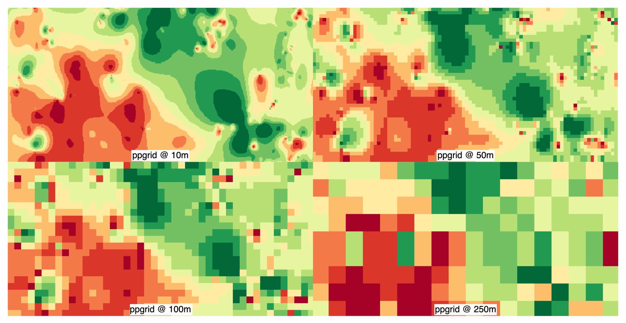
A single 100K-point dataset rendered at four resolutions. The adaptive mipmap pyramid fills sparse regions from coarser layers, so you get a continuous surface instead of patchy gaps.
What it does
You have N points with (longitude, latitude, value). You want a raster where every cell within a specified distance of real data carries an interpolated value, and everything else is nodata.
Standard IDW in QGIS or ArcGIS is O(N*M) (~14 hours for 16M points). This tool uses pull-push mipmap interpolation to reduce cost to O(M), independent of N.
How it works
Pull-Push (mipmap) Interpolation
Based on Gortler et al. 1996 (Lumigraph) and Kraus 2009.
Once points are snapped to a grid, IDW is exactly a normalised convolution:
z = (S ⊛ K) / (C ⊛ K) K(r) = r^-p
Pull-push evaluates this across a mipmap pyramid so cost is O(M), independent of N.
Steps:
- Points are binned into
S(sum of transformed values) andC(count) grids - A mipmap pyramid is built by repeated 2x2 block sums
- The coarsest level seeds the interpolation
- Descending the pyramid, each level blends local estimate vs upsampled parent
- Local confidence is
min(C/saturation, 1). Dense cells trust themselves, sparse cells inherit - A summed-area table (
box_count) provides an exact radius fill cap
Output bands:
- Value: int16, 0-100 percentile,
percentile = DN/scale - Support km: int16,
support_km = 2^(DN/8), effective spatial scale of estimate
Working CRS: EPSG:6933 (Wagner VII) by default. Global equal-area, metres are true. Configurable via --work-crs.
Output CRS: EPSG:3857 (Web Mercator) by default. Configurable via --out-crs.
Calibration (optional)
Before interpolation, the tool can:
- Choose a transform. Tests identity/log10/sqrt/percentile and picks the one with highest intraclass correlation across coarse scales
- Derive a fill cap. Spatially blocked cross-validation to find the honest distance beyond which interpolation has no skill
- Save calibration.json. Contains the percentile-to-value lookup table for decoding the output raster back to real units
Install
Requires Python 3.11+ (older interpreters fail the pip resolver with a bare error).
pip install ppgrid
For Parquet support:
pip install ppgrid[parquet]
Or from source:
git clone https://github.com/marzukia/ppgrid.git
cd ppgrid
uv sync
Quick Start
ppgrid data.csv --value-col price --res 500 --cap-km 10 --skip-calibration
This reads data.csv, interpolates the price column at 500m resolution with a 10km fill cap, and writes value.tif + support_km.tif to out/.
Usage
# Quick run (skip calibration)
ppgrid data.csv --value-col premium --res 500 --cap-km 64 --skip-calibration

# Full run with calibration (saves calibration.json)
ppgrid data.csv --value-col premium --res 100 --cap-km auto

# Custom projection and params
ppgrid data.csv --value-col premium --res 100 --cap-km 25 --transform log10 --workers 8

# Reuse existing calibration
ppgrid data.csv --value-col premium --calibration calibration.json

# Round output percentiles to a step (e.g. 5 -> 90/95/100) for clean vectorisation
ppgrid data.csv --value-col premium --res 100 --cap-km 25 --percentile-step 5
CLI Options
| Flag | Default | Description |
|---|---|---|
input | (required) | CSV or Parquet input path |
-o, --out | out/ | Output directory |
--value-col | value | Value column name |
--lng-col | longitude | Longitude column name |
--lat-col | latitude | Latitude column name |
--res | 500.0 | Cell size in metres |
--cap-km | auto | Fill cap km, or 'auto' (blocked-CV derived) |
--transform | auto | auto, identity, log10, sqrt, percentile |
--saturation | 1.0 | Counts for a cell to fully self-trust |
--block | 2048 | Block size in cells |
--workers | 4 | Number of parallel workers |
--scale | 100.0 | DN = percentile * scale |
--percentile-step | (none) | Round output percentiles to the nearest step (e.g. 5 -> 90/95/100) |
--compress | ZSTD | GeoTIFF compression |
--calibration | (none) | Path to existing calibration.json |
--calib-max-points | 2000000 | Max points to use for calibration |
--src-crs | 4326 | Input coordinate reference system |
--work-crs | 6933 | Working CRS for interpolation (equal-area) |
--out-crs | 3857 | Output CRS for final GeoTIFF |
--skip-calibration | False | Skip calibration, use defaults |
Decoding the output
The value band stores percentiles, not raw values. To convert back to real units, use the calibration.json saved in the output folder:
import json, numpy as np, rasterio

with open("calibration.json") as f:
    quantiles = np.array(json.load(f)["percentile_quantiles"])

with rasterio.open("value.tif") as r:
    percentiles = np.array(r.read(1), copy=True) / 100.0

real_values = np.interp(percentiles, np.linspace(0, 100, len(quantiles)), quantiles)
Benchmarks
Head-to-head on a 100K-point synthetic dataset (M4 MacBook Pro, 24GB) against the traditional GDAL path:
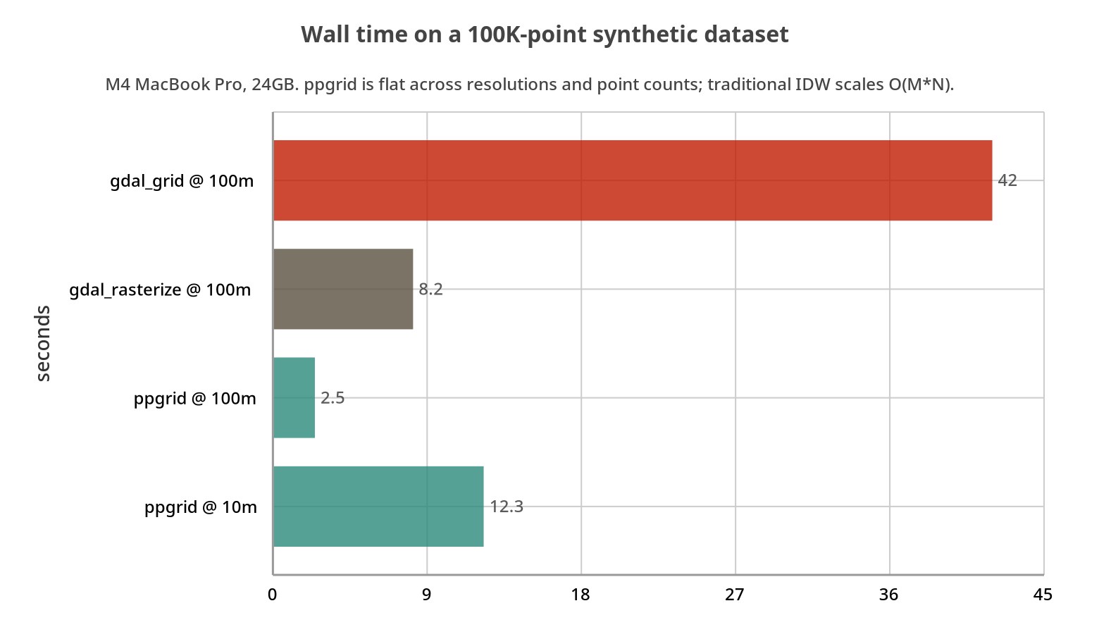
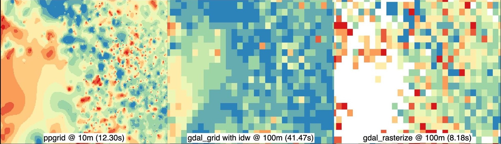
ppgrid at 100m is ~17x faster than gdal_grid and ~3x faster than gdal_rasterize at the same resolution, and it can run 10x finer (10m) in under 13 seconds.
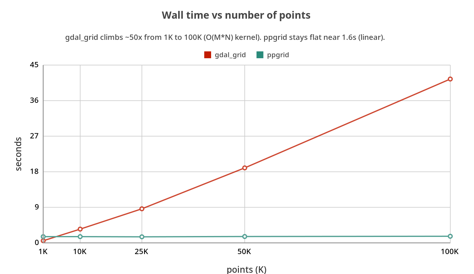
The reason is the scaling behaviour. As the point count grows, gdal_grid climbs ~50x from 1K to 100K points (the O(M*N) kernel), while ppgrid stays flat near 1.6s because each point is binned once and the rest is linear over raster cells:
Resolution sweep
Melbourne Housing dataset (13,580 points) at various resolutions on the same machine:
| Resolution | Wall Time | File Size |
|---|---|---|
| 10m | 26.6s | 27.3 MB |
| 25m | 4.0s | 6.8 MB |
| 50m | 1.3s | 2.3 MB |
| 100m | 0.8s | 749 KB |
| 250m | 0.6s | 159 KB |
| 500m | 0.6s | 49 KB |
Example Outputs
ppgrid against gdal_grid + IDW and gdal_rasterize on the same data. Left is ppgrid, middle is gdal_grid with IDW, right is gdal_rasterize:
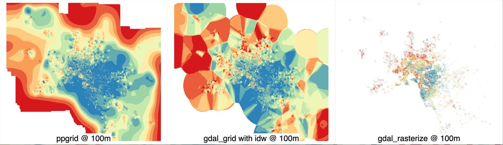
Zoomed in. ppgrid stays continuous where the grid-based methods produce Voronoi-style polygons and patchy gaps:
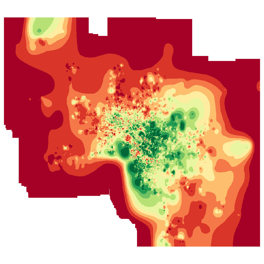
Melbourne Housing interpolated at 10m, full extent:
Data
data/melb_houses.csv: 13,580 Melbourne property sales with latitude, longitude, and price. Sourced from the Melbourne Housing Snapshot (CC BY-NC-SA 4.0).
data/all_equakes.csv: 44,376 earthquake events from Jan-Aug 2026, mag >= 1.5.
Data Lineage
| Step | Description |
|---|---|
| Source | USGS Earthquake Hazards Program |
| API | FDSN Event Web Service |
| Download | Batched CSV requests by month, minmagnitude=1.5, starttime=2026-01-01, endtime=2026-08-08 |
| Processing | Concatenated monthly CSVs (deduplicated header) into single file |
| License | Public Domain (USGS federal data) |
Columns Used
latitude/longitude: spatial coordinates (WGS 84)mag: earthquake magnitude (continuous, for interpolation)depth: focal depth in km (optional value layer)time: event timestamp (ISO 8601)
Contributors


Similar repos


Languages
Python
100.0%
Fast continent-scale raster interpolation for scattered point data. Turns millions of geolocated points into gapless GeoTIFF in minutes using IDW and pull-push mipmap algorithms. No GPU required.
See the codeSee what people are saying
README
ppgrid - Pull-Push Scattered-Data Interpolation
Fast, continent-scale raster interpolation for scattered point data. Turns tens of millions of geolocated points into a pair of GeoTIFFs in minutes on a single machine. No GPU needed.
A single 100K-point dataset rendered at four resolutions. The adaptive mipmap pyramid fills sparse regions from coarser layers, so you get a continuous surface instead of patchy gaps.
What it does
You have N points with (longitude, latitude, value). You want a raster where every cell within a specified distance of real data carries an interpolated value, and everything else is nodata.
Standard IDW in QGIS or ArcGIS is O(N*M) (~14 hours for 16M points). This tool uses pull-push mipmap interpolation to reduce cost to O(M), independent of N.
How it works
Pull-Push (mipmap) Interpolation
Based on Gortler et al. 1996 (Lumigraph) and Kraus 2009.
Once points are snapped to a grid, IDW is exactly a normalised convolution:
z = (S ⊛ K) / (C ⊛ K) K(r) = r^-p
Pull-push evaluates this across a mipmap pyramid so cost is O(M), independent of N.
Steps:
- Points are binned into
S(sum of transformed values) andC(count) grids - A mipmap pyramid is built by repeated 2x2 block sums
- The coarsest level seeds the interpolation
- Descending the pyramid, each level blends local estimate vs upsampled parent
- Local confidence is
min(C/saturation, 1). Dense cells trust themselves, sparse cells inherit - A summed-area table (
box_count) provides an exact radius fill cap
Output bands:
- Value: int16, 0-100 percentile,
percentile = DN/scale - Support km: int16,
support_km = 2^(DN/8), effective spatial scale of estimate
Working CRS: EPSG:6933 (Wagner VII) by default. Global equal-area, metres are true. Configurable via --work-crs.
Output CRS: EPSG:3857 (Web Mercator) by default. Configurable via --out-crs.
Calibration (optional)
Before interpolation, the tool can:
- Choose a transform. Tests identity/log10/sqrt/percentile and picks the one with highest intraclass correlation across coarse scales
- Derive a fill cap. Spatially blocked cross-validation to find the honest distance beyond which interpolation has no skill
- Save calibration.json. Contains the percentile-to-value lookup table for decoding the output raster back to real units
Install
Requires Python 3.11+ (older interpreters fail the pip resolver with a bare error).
pip install ppgrid
For Parquet support:
pip install ppgrid[parquet]
Or from source:
git clone https://github.com/marzukia/ppgrid.git
cd ppgrid
uv sync
Quick Start
ppgrid data.csv --value-col price --res 500 --cap-km 10 --skip-calibration
This reads data.csv, interpolates the price column at 500m resolution with a 10km fill cap, and writes value.tif + support_km.tif to out/.
Usage
# Quick run (skip calibration)
ppgrid data.csv --value-col premium --res 500 --cap-km 64 --skip-calibration

# Full run with calibration (saves calibration.json)
ppgrid data.csv --value-col premium --res 100 --cap-km auto

# Custom projection and params
ppgrid data.csv --value-col premium --res 100 --cap-km 25 --transform log10 --workers 8

# Reuse existing calibration
ppgrid data.csv --value-col premium --calibration calibration.json

# Round output percentiles to a step (e.g. 5 -> 90/95/100) for clean vectorisation
ppgrid data.csv --value-col premium --res 100 --cap-km 25 --percentile-step 5
CLI Options
| Flag | Default | Description |
|---|---|---|
input | (required) | CSV or Parquet input path |
-o, --out | out/ | Output directory |
--value-col | value | Value column name |
--lng-col | longitude | Longitude column name |
--lat-col | latitude | Latitude column name |
--res | 500.0 | Cell size in metres |
--cap-km | auto | Fill cap km, or 'auto' (blocked-CV derived) |
--transform | auto | auto, identity, log10, sqrt, percentile |
--saturation | 1.0 | Counts for a cell to fully self-trust |
--block | 2048 | Block size in cells |
--workers | 4 | Number of parallel workers |
--scale | 100.0 | DN = percentile * scale |
--percentile-step | (none) | Round output percentiles to the nearest step (e.g. 5 -> 90/95/100) |
--compress | ZSTD | GeoTIFF compression |
--calibration | (none) | Path to existing calibration.json |
--calib-max-points | 2000000 | Max points to use for calibration |
--src-crs | 4326 | Input coordinate reference system |
--work-crs | 6933 | Working CRS for interpolation (equal-area) |
--out-crs | 3857 | Output CRS for final GeoTIFF |
--skip-calibration | False | Skip calibration, use defaults |
Decoding the output
The value band stores percentiles, not raw values. To convert back to real units, use the calibration.json saved in the output folder:
import json, numpy as np, rasterio

with open("calibration.json") as f:
    quantiles = np.array(json.load(f)["percentile_quantiles"])

with rasterio.open("value.tif") as r:
    percentiles = np.array(r.read(1), copy=True) / 100.0

real_values = np.interp(percentiles, np.linspace(0, 100, len(quantiles)), quantiles)
Benchmarks
Head-to-head on a 100K-point synthetic dataset (M4 MacBook Pro, 24GB) against the traditional GDAL path:
ppgrid at 100m is ~17x faster than gdal_grid and ~3x faster than gdal_rasterize at the same resolution, and it can run 10x finer (10m) in under 13 seconds.
The reason is the scaling behaviour. As the point count grows, gdal_grid climbs ~50x from 1K to 100K points (the O(M*N) kernel), while ppgrid stays flat near 1.6s because each point is binned once and the rest is linear over raster cells:
Resolution sweep
Melbourne Housing dataset (13,580 points) at various resolutions on the same machine:
| Resolution | Wall Time | File Size |
|---|---|---|
| 10m | 26.6s | 27.3 MB |
| 25m | 4.0s | 6.8 MB |
| 50m | 1.3s | 2.3 MB |
| 100m | 0.8s | 749 KB |
| 250m | 0.6s | 159 KB |
| 500m | 0.6s | 49 KB |
Example Outputs
ppgrid against gdal_grid + IDW and gdal_rasterize on the same data. Left is ppgrid, middle is gdal_grid with IDW, right is gdal_rasterize:
Zoomed in. ppgrid stays continuous where the grid-based methods produce Voronoi-style polygons and patchy gaps:
Melbourne Housing interpolated at 10m, full extent:
Data
data/melb_houses.csv: 13,580 Melbourne property sales with latitude, longitude, and price. Sourced from the Melbourne Housing Snapshot (CC BY-NC-SA 4.0).
data/all_equakes.csv: 44,376 earthquake events from Jan-Aug 2026, mag >= 1.5.
Data Lineage
| Step | Description |
|---|---|
| Source | USGS Earthquake Hazards Program |
| API | FDSN Event Web Service |
| Download | Batched CSV requests by month, minmagnitude=1.5, starttime=2026-01-01, endtime=2026-08-08 |
| Processing | Concatenated monthly CSVs (deduplicated header) into single file |
| License | Public Domain (USGS federal data) |
Columns Used
latitude/longitude: spatial coordinates (WGS 84)mag: earthquake magnitude (continuous, for interpolation)depth: focal depth in km (optional value layer)time: event timestamp (ISO 8601)
Similar repos
Contributors
Languages
Python
100.0%