
Editable ipywidgets tables of elements in series, with live computed columns, unit toggles and plots.
Python
0
5 commits
updated Sep 27, 2026
See what people are saying
README
ipyrowtable
Editable ipywidgets tables for problems made of elements
in series: wall layers, pipe segments, cable runs, process stages. You describe the columns
and write a compute function; ipyrowtable gives a table where Jupyter users add and remove
rows, edit inputs, see computed results update immediately, and easily use the configured inputs
in downstream cells.
What sets it apart from a general-purpose data grid:
- Every cell is a real widget. Dropdowns, number boxes and text boxes in the table itself, with add and remove buttons per row.
- Values between rows. A
NodeColumnholds the n + 1 values at the joints of n elements (interface temperatures, joint pressures, node voltages), with editable boundary conditions at either end. - Unit systems. A toggle switches everything shown between, say, SI and Imperial. Values are stored in your base units, so switching never changes the physics or drifts.
- Live plots.
LiveFigurekeeps a matplotlib figure in step with the table. - Saved between sessions. A table can keep its inputs across kernel restarts, making it a friendlier alternative to a hard-coded dict of inputs.
It suits small, carefully entered inputs: tens of rows, not thousands. For large data, use a grid such as ipydatagrid or Panel's Tabulator.
Install
pip install ipyrowtable            # the table
pip install "ipyrowtable[plot]"    # plus matplotlib, for LiveFigure and the conduction example
Needs Python 3.10+ and ipywidgets 8.1+. It uses only standard widgets, with no custom JavaScript, so it works wherever ipywidgets does: JupyterLab, Jupyter Notebook, VS Code, Voilà.
Try it
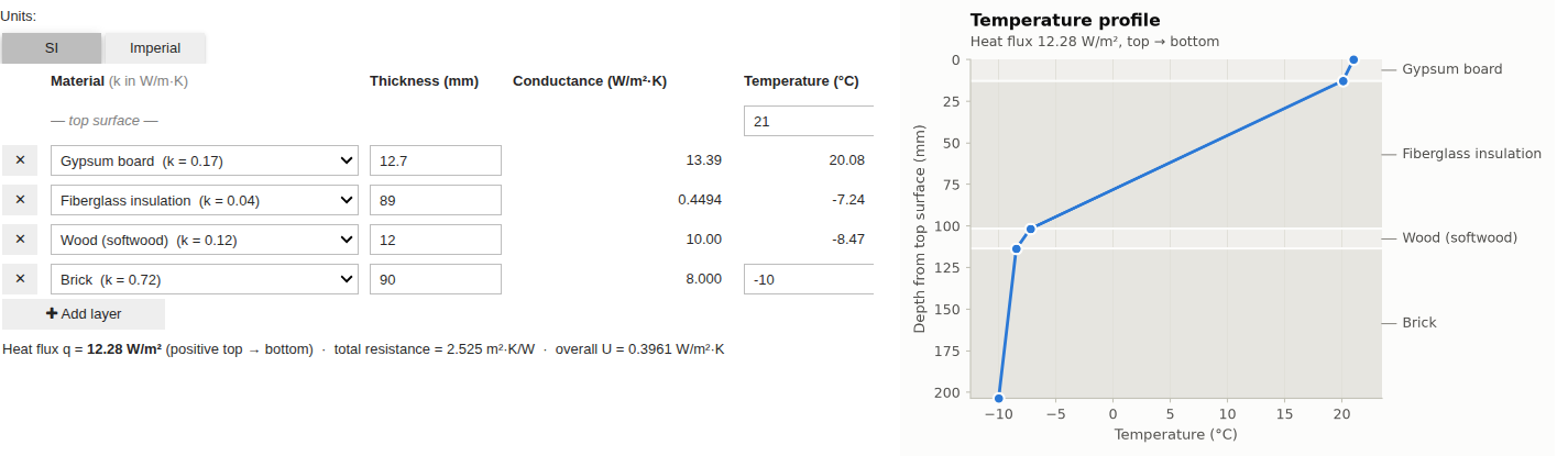
A complete application ships with the package: steady conduction through a plane composite wall, with an SI / Imperial toggle and a temperature-profile plot.
from ipyrowtable.examples.conduction import layer_stack_app

layer_stack_app(layers=[("Gypsum board", 12.7), ("Fiberglass insulation", 89), ("Brick", 90)],
                T_top=21, T_bottom=-10)
Quick start
Voltage along a cable run. Each row is a segment; the voltage at each joint is computed from the source voltage (an editable boundary value) and the load current (a parameter that applies to the whole run).
import numpy as np
from ipyrowtable import ChoiceColumn, NodeColumn, NumberColumn, OutputColumn, RowTable

OHM_PER_M = {"14 AWG": 0.008286, "12 AWG": 0.005211, "10 AWG": 0.003277}  # copper, 20 °C

def voltage_drop(inputs):
    ohm_per_m = np.array([OHM_PER_M[g] for g in inputs.column("gauge")])
    drop = 2 * inputs.params["current"] * ohm_per_m * inputs.column("length")  # out and back
    V_source = inputs.edges["voltage"][0]
    return {"drop": drop, "voltage": V_source - np.concatenate(([0.0], np.cumsum(drop)))}

cable = RowTable(
    columns=[
        ChoiceColumn("gauge", "Wire", options=OHM_PER_M),
        NumberColumn("length", "Length (m)", default=10.0, min=0),
        OutputColumn("drop", "Drop (V)"),
        NodeColumn("voltage", "Voltage (V)", inputs="first", first_default=120.0),
    ],
    compute=voltage_drop,
    parameters=[NumberColumn("current", "Current (A)", default=15.0)],
    leading_label="— source —",
    item_name="segment",
)
cable
cable.results["voltage"] holds the latest values, and cable.results.records() gives one
dict per row, ready for pandas.DataFrame.
Concepts
Columns
| Column | Kind | Per row |
|---|---|---|
ChoiceColumn | input | a dropdown; options can carry data, like a material's conductivity |
NumberColumn | input | a number, optionally unit-aware (quantity=) and bounded (min=, max=) |
TextColumn | input | free text, such as a name or tag |
OutputColumn | output | one computed value |
NodeColumn | output | the value at the row's bottom or outlet face; the value at the top or inlet goes in a leading row |
Headers can include units: "Thickness ({unit})" shows the column's own unit, and
"k in {conductivity}" shows any other quantity's unit.
Input columns can also be parameters, shown above the table for values that apply to the
whole problem. To add a new input type, subclass InputColumn and implement create_widget.
The 03_extending notebook adds a whole-number column this way.
Values between rows
A NodeColumn holds n + 1 values for n rows. Use inputs= to say which ends are
editable:
("first", "last")for both ends, like the two surface temperatures of a wall"first"for the inlet only, like a supply pressure"last"for the outlet only()for neither
Your compute function receives the boundary values as inputs.edges[key] and returns all
n + 1 values, including the ends.
Units
from ipyrowtable import Unit, UnitSystem

SI = UnitSystem("SI", {"length": Unit("mm", 1000.0), "temperature": Unit("°C")})
IMPERIAL = UnitSystem("Imperial", {"length": Unit("in", 1 / 0.0254),
                                   "temperature": Unit("°F", 1.8, 32.0)})
A Unit converts with display = base × scale + offset. Your compute function always works
in base units (metres and °C here). Pass unit_systems=[SI, IMPERIAL] to get a toggle.
Defaults can be given per system, such as default={"SI": 10, "Imperial": 0.5}, so new rows
start at round numbers in whichever units are showing.
The compute function and results
compute(inputs) receives:
inputs.rows: a list of dicts, one per rowinputs.column(key): one column as an arrayinputs.edges: the NodeColumn boundary valuesinputs.params: the parameters
All of them are in base units. It returns {column key: values}, and any extra keys (totals,
fluxes) are kept too. If it raises ValueError("message"), the message appears in place of
the results.
After every change:
table.results[key]gives values in base units, andtable.results.display(key)gives them in the units shown.table.results.records()gives one dict per row.table.on_update(callback)runs your code with the results, or withNonewhile the inputs are invalid.table.errorsays what went wrong, if anything did.
Saving inputs between sessions
cable = RowTable(..., rows=[...], persist="feeder")
With a persist key, the table saves its inputs whenever they change and restores them when
a table with the same key is created again, for example after a kernel restart. The inputs
are the rows, boundary values, parameters, and the unit system that was showing.
rows, edges, params and units then become the initial values. They're used:
- when nothing has been saved yet;
- when the saved inputs can't be used, for example because an option no longer exists (the
table says why, and keeps the old file as a
.bakcopy before replacing it); - by the Reset button, which asks for a second click first.
Where the inputs go:
- By default, into
<notebook name>.ipyrowtable.jsonnext to the notebook. If the notebook can't be identified, they go intoipyrowtable.jsonin the working folder. The note under the table names the file. persist_file=picks a different file. One file can hold many tables, each under its own key.- Values are stored as plain JSON in base units, so it doesn't matter which unit system was showing.
They go in a file rather than the notebook's metadata because the kernel can't write notebook metadata.
To always start from the initial values, leave out persist. The environment variable
IPYROWTABLE_PERSIST=off turns saving off for every table, which is useful for batch runs
that must start from known inputs. table.get_inputs() and table.set_inputs(snapshot) let
you keep and load snapshots yourself, such as several named designs.
Plots
from ipyrowtable import LiveFigure, side_by_side

def draw(fig, results):
    ax = fig.add_subplot()
    ax.plot(results["voltage"], marker="o")

side_by_side(cable, LiveFigure(cable, draw=draw))
Styling
Every part carries a CSS class you can style:
ipyrowtable-grid,ipyrowtable-add,ipyrowtable-reset,ipyrowtable-message,ipyrowtable-persistipyrowtable-<key>on each column's cells
Examples
The examples/ folder has four notebooks:
- 01_getting_started: a first table, values between rows, a live plot, driving a table from code.
- 02_plane_wall_conduction: the conduction app: units, reading results, plugging in your own solver.
- 03_extending: pipes in series (Darcy–Weisbach). Covers your own unit systems, a custom
column type, parameters,
on_update, and styling. - 04_saving_inputs: keeping a table's inputs between sessions: initial values, the saved file, named snapshots, resetting, and turning saving off.
FAQ
In VS Code, a table shows "Failed to load model class …" instead of rendering
This can happen the first time a notebook runs in VS Code's Jupyter extension, when a table is created in one cell and displayed in a later one. It comes from how VS Code loads its widget support: widgets created before VS Code has finished loading it can fail to render. It isn't caused by ipyrowtable, which uses only standard ipywidgets. Seen with the Jupyter extension 2025.9.1 on Windows.
- To fix it: re-run the cell that creates the table, then the cell that displays it.
Development
See CONTRIBUTING.md for setup, the test suite (including real-browser tests) and releasing.
License
MIT
Similar repos


Languages
Python
100.0%
Editable ipywidgets tables of elements in series, with live computed columns, unit toggles and plots.
Python
0
5 commits
updated Sep 27, 2026
See what people are saying
README
ipyrowtable
Editable ipywidgets tables for problems made of elements
in series: wall layers, pipe segments, cable runs, process stages. You describe the columns
and write a compute function; ipyrowtable gives a table where Jupyter users add and remove
rows, edit inputs, see computed results update immediately, and easily use the configured inputs
in downstream cells.
What sets it apart from a general-purpose data grid:
- Every cell is a real widget. Dropdowns, number boxes and text boxes in the table itself, with add and remove buttons per row.
- Values between rows. A
NodeColumnholds the n + 1 values at the joints of n elements (interface temperatures, joint pressures, node voltages), with editable boundary conditions at either end. - Unit systems. A toggle switches everything shown between, say, SI and Imperial. Values are stored in your base units, so switching never changes the physics or drifts.
- Live plots.
LiveFigurekeeps a matplotlib figure in step with the table. - Saved between sessions. A table can keep its inputs across kernel restarts, making it a friendlier alternative to a hard-coded dict of inputs.
It suits small, carefully entered inputs: tens of rows, not thousands. For large data, use a grid such as ipydatagrid or Panel's Tabulator.
Install
pip install ipyrowtable            # the table
pip install "ipyrowtable[plot]"    # plus matplotlib, for LiveFigure and the conduction example
Needs Python 3.10+ and ipywidgets 8.1+. It uses only standard widgets, with no custom JavaScript, so it works wherever ipywidgets does: JupyterLab, Jupyter Notebook, VS Code, Voilà.
Try it
A complete application ships with the package: steady conduction through a plane composite wall, with an SI / Imperial toggle and a temperature-profile plot.
from ipyrowtable.examples.conduction import layer_stack_app

layer_stack_app(layers=[("Gypsum board", 12.7), ("Fiberglass insulation", 89), ("Brick", 90)],
                T_top=21, T_bottom=-10)
Quick start
Voltage along a cable run. Each row is a segment; the voltage at each joint is computed from the source voltage (an editable boundary value) and the load current (a parameter that applies to the whole run).
import numpy as np
from ipyrowtable import ChoiceColumn, NodeColumn, NumberColumn, OutputColumn, RowTable

OHM_PER_M = {"14 AWG": 0.008286, "12 AWG": 0.005211, "10 AWG": 0.003277}  # copper, 20 °C

def voltage_drop(inputs):
    ohm_per_m = np.array([OHM_PER_M[g] for g in inputs.column("gauge")])
    drop = 2 * inputs.params["current"] * ohm_per_m * inputs.column("length")  # out and back
    V_source = inputs.edges["voltage"][0]
    return {"drop": drop, "voltage": V_source - np.concatenate(([0.0], np.cumsum(drop)))}

cable = RowTable(
    columns=[
        ChoiceColumn("gauge", "Wire", options=OHM_PER_M),
        NumberColumn("length", "Length (m)", default=10.0, min=0),
        OutputColumn("drop", "Drop (V)"),
        NodeColumn("voltage", "Voltage (V)", inputs="first", first_default=120.0),
    ],
    compute=voltage_drop,
    parameters=[NumberColumn("current", "Current (A)", default=15.0)],
    leading_label="— source —",
    item_name="segment",
)
cable
cable.results["voltage"] holds the latest values, and cable.results.records() gives one
dict per row, ready for pandas.DataFrame.
Concepts
Columns
| Column | Kind | Per row |
|---|---|---|
ChoiceColumn | input | a dropdown; options can carry data, like a material's conductivity |
NumberColumn | input | a number, optionally unit-aware (quantity=) and bounded (min=, max=) |
TextColumn | input | free text, such as a name or tag |
OutputColumn | output | one computed value |
NodeColumn | output | the value at the row's bottom or outlet face; the value at the top or inlet goes in a leading row |
Headers can include units: "Thickness ({unit})" shows the column's own unit, and
"k in {conductivity}" shows any other quantity's unit.
Input columns can also be parameters, shown above the table for values that apply to the
whole problem. To add a new input type, subclass InputColumn and implement create_widget.
The 03_extending notebook adds a whole-number column this way.
Values between rows
A NodeColumn holds n + 1 values for n rows. Use inputs= to say which ends are
editable:
("first", "last")for both ends, like the two surface temperatures of a wall"first"for the inlet only, like a supply pressure"last"for the outlet only()for neither
Your compute function receives the boundary values as inputs.edges[key] and returns all
n + 1 values, including the ends.
Units
from ipyrowtable import Unit, UnitSystem

SI = UnitSystem("SI", {"length": Unit("mm", 1000.0), "temperature": Unit("°C")})
IMPERIAL = UnitSystem("Imperial", {"length": Unit("in", 1 / 0.0254),
                                   "temperature": Unit("°F", 1.8, 32.0)})
A Unit converts with display = base × scale + offset. Your compute function always works
in base units (metres and °C here). Pass unit_systems=[SI, IMPERIAL] to get a toggle.
Defaults can be given per system, such as default={"SI": 10, "Imperial": 0.5}, so new rows
start at round numbers in whichever units are showing.
The compute function and results
compute(inputs) receives:
inputs.rows: a list of dicts, one per rowinputs.column(key): one column as an arrayinputs.edges: the NodeColumn boundary valuesinputs.params: the parameters
All of them are in base units. It returns {column key: values}, and any extra keys (totals,
fluxes) are kept too. If it raises ValueError("message"), the message appears in place of
the results.
After every change:
table.results[key]gives values in base units, andtable.results.display(key)gives them in the units shown.table.results.records()gives one dict per row.table.on_update(callback)runs your code with the results, or withNonewhile the inputs are invalid.table.errorsays what went wrong, if anything did.
Saving inputs between sessions
cable = RowTable(..., rows=[...], persist="feeder")
With a persist key, the table saves its inputs whenever they change and restores them when
a table with the same key is created again, for example after a kernel restart. The inputs
are the rows, boundary values, parameters, and the unit system that was showing.
rows, edges, params and units then become the initial values. They're used:
- when nothing has been saved yet;
- when the saved inputs can't be used, for example because an option no longer exists (the
table says why, and keeps the old file as a
.bakcopy before replacing it); - by the Reset button, which asks for a second click first.
Where the inputs go:
- By default, into
<notebook name>.ipyrowtable.jsonnext to the notebook. If the notebook can't be identified, they go intoipyrowtable.jsonin the working folder. The note under the table names the file. persist_file=picks a different file. One file can hold many tables, each under its own key.- Values are stored as plain JSON in base units, so it doesn't matter which unit system was showing.
They go in a file rather than the notebook's metadata because the kernel can't write notebook metadata.
To always start from the initial values, leave out persist. The environment variable
IPYROWTABLE_PERSIST=off turns saving off for every table, which is useful for batch runs
that must start from known inputs. table.get_inputs() and table.set_inputs(snapshot) let
you keep and load snapshots yourself, such as several named designs.
Plots
from ipyrowtable import LiveFigure, side_by_side

def draw(fig, results):
    ax = fig.add_subplot()
    ax.plot(results["voltage"], marker="o")

side_by_side(cable, LiveFigure(cable, draw=draw))
Styling
Every part carries a CSS class you can style:
ipyrowtable-grid,ipyrowtable-add,ipyrowtable-reset,ipyrowtable-message,ipyrowtable-persistipyrowtable-<key>on each column's cells
Examples
The examples/ folder has four notebooks:
- 01_getting_started: a first table, values between rows, a live plot, driving a table from code.
- 02_plane_wall_conduction: the conduction app: units, reading results, plugging in your own solver.
- 03_extending: pipes in series (Darcy–Weisbach). Covers your own unit systems, a custom
column type, parameters,
on_update, and styling. - 04_saving_inputs: keeping a table's inputs between sessions: initial values, the saved file, named snapshots, resetting, and turning saving off.
FAQ
In VS Code, a table shows "Failed to load model class …" instead of rendering
This can happen the first time a notebook runs in VS Code's Jupyter extension, when a table is created in one cell and displayed in a later one. It comes from how VS Code loads its widget support: widgets created before VS Code has finished loading it can fail to render. It isn't caused by ipyrowtable, which uses only standard ipywidgets. Seen with the Jupyter extension 2025.9.1 on Windows.
- To fix it: re-run the cell that creates the table, then the cell that displays it.
Development
See CONTRIBUTING.md for setup, the test suite (including real-browser tests) and releasing.
License
MIT
Similar repos
Languages
Python
100.0%