Reproducing, then improving MiniPile with PyTorch and HuggingFace
Python
2
297 commits
updated Feb 25, 2025
MiniCorpus reproduces and investigates enhancements for MiniPile (Kaddour, Jean. 2023), a distilled subset of The Pile Deduplicated, related to (Gao, et al. 2020). MiniPile enables efficient LLM training using two orders of magnitude less data while aiming to maintain competitive performance compared to models trained on the full deduplicated Pile.
MiniCorpus covers the following steps:
Key objectives of this project:
The findings and implications of this project are presented at the end of the Conclusion section.
The produced models and datasets can be found on HuggingFace and are additionally listed further below in the Datasets and Models sections.
conda env create -f minicorpus.yaml.Instructions for running each script in this repository are provided at the end of each respective script.
01_get_piles.ipynb.03_embed_pile_dedup_turbo.py.03_embed_pile_dedup_turbo.py starts with the actual processing, run 03_cluster_pile_embed.py to cluster the embeddings. The clustering script was built to run the fitting of k-Means in parallel with the embedding script producing new embeddings.03_cluster_pile_embed.py will store the centroids and automatically start clustering the embeddings.cluster_info_for_inspection.json in the MiniPile_BatchKMeans folder for manual cluster exclusion.03_sort_pile_clusters.py to have the clustered embeddings sorted by their assigned cluster into dedicated jsonl files.03_distill_pile_embed.py or either of the 04_distill_pile_embed_*.py scripts to sample a flavor of MiniPile from the embedded Pile.03_train_160M_*.py or 03_train_1.4B_*.py or either of the 04_train_160M_*.py or 04_train_1.4B_*.py to train a model on your chosen MiniPile flavor. You may need to uncomment the download function inside the training script to have it download the untrained base model first.00_pile_pusher.py to push any of the artifacts you produced to your HuggingFace account.Reproduction of MiniPile's assembly is necessary to form a basis for attempts at improving it.
The reproduction process is split across three chapters.
Files belonging to these chapters are prefixed with 01_, 02_, and 03_ respectively.
Jupyter Notebooks are added for each chapter for documentation and guidance.
01 is concerned with downloading The Pile Deduplicated and the original MiniPile as baseline. Be sure to have enough disk space available.
01_get_piles.ipynb.02 regards training a Pythia 160M model on the original MiniPile and benchmarking it in zero-shot settings with the EleutherAI LM Evaluation Harness.
02_eval_160M.ipynb.03 is about reproducing MiniPile from scratch. This includes embedding the deduplicated Pile, clustering the embeddings, and sampling a MiniPile from the clusters in accordance with the MiniPile paper.We deem our reproduction of MiniPile successful.
However, we had to make compromises and assumptions:
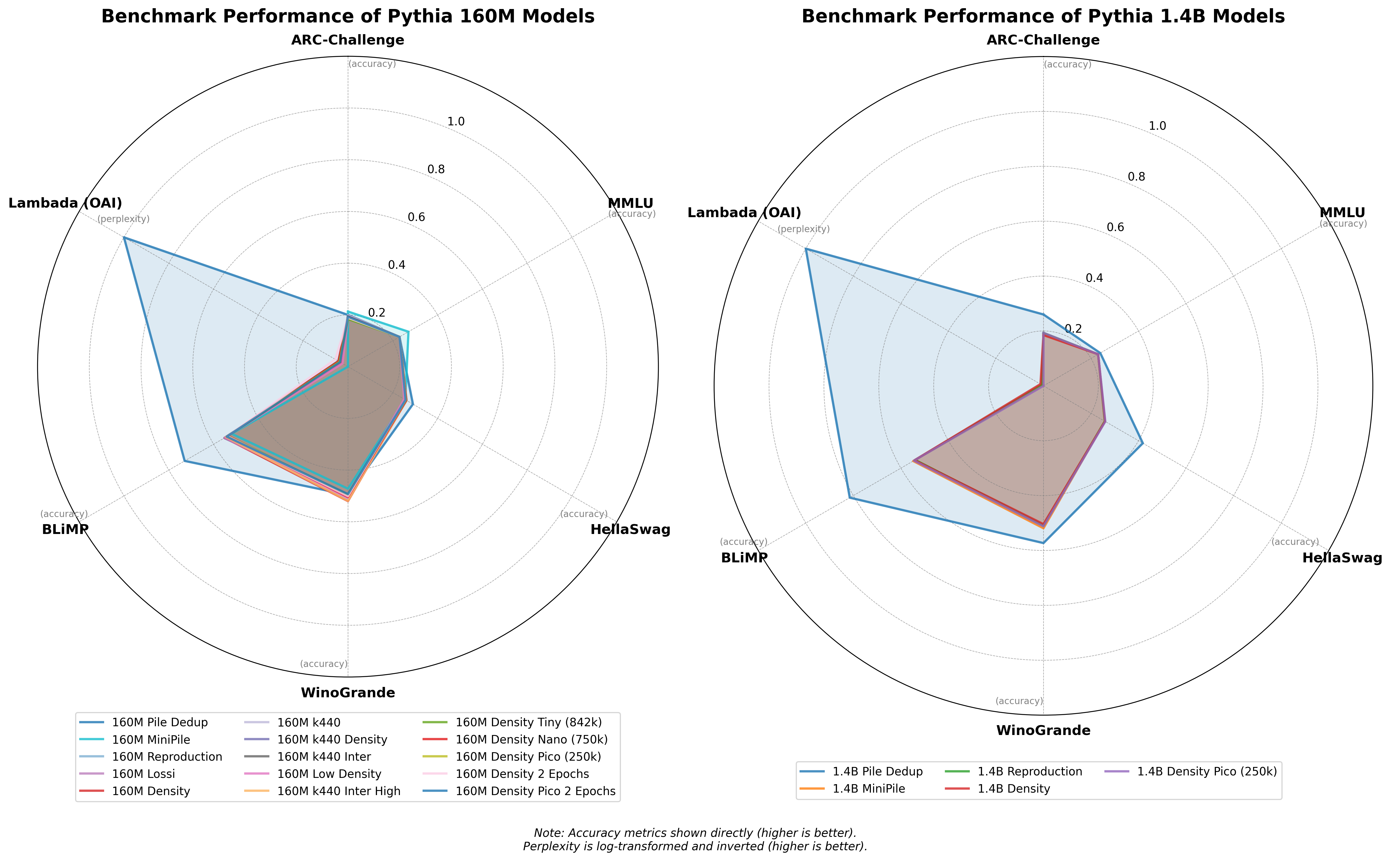
The reproduction dataset showed deviations from the benchmark results produced for MiniPile. These were observed both in the positive and negative direction on the Pythia 160M architecture. Most strongly deviating results were witnessed on ARC-Challenge (-10.9%) and MMLU (-15%) respectively, while HellaSwag (+1.72%), WinoGrande (+8.52%) and BLiMP (+5.53%) improved.
Notably, Lambada perplexity scores were reduced by 38.9% on Lambada OpenAI and 55% on Lambada Std. This indicates a potential tilt in the produced dataset in a slightly different direction content-wise, compared to the original MiniPile, due to derivation of embeddings or cluster selection. The small performance improvements witnessed on a majority of the benchmarks lead us to conclude that the reproduction shows characteristics in accordance with the paper's results and is within the margin of error. The deviations are sufficiently explainable by the need for speed (E5-Base-4k) and the human-guided cluseter exlcusion that can't be reproduced in detail. Even with our assumptions and changes to the methodology in place, we do not witness a fundamental departure from the paper's results overall. We therefore deem the reproduction successful.
The MiniPile pipeline can be improved by finding a way of sampling a data subset that is ideally even smaller than MiniPile and yet more representative of the original Pile Deduplicated.
Ultimately resulting in success, several attempts were undertaken to improve the MiniPile pipeline for these objectives.
All individual ideas are documented extensively in the fourth chapter's Jupyter Notebook 04_improve_minipile.ipynb, which lays out the intentions and reasonings more thoroughly. The following ideas and ablation studies were conducted:
04_distill_pile_embed_idea_1_proportionate.py)04_distill_pile_embed_idea_2_lossi_1.py and 04_distill_pile_embed_idea_2_lossi_2.py)04_distill_pile_embed_idea_3_density.py)04_distill_pile_embed_idea_3.1_density_low.py)04_cluster_pile_embed_idea_4_double.py, 04_distill_pile_embed_idea_4_k440.py)04_distill_pile_embed_idea_5_k440_density.py)04_distill_pile_embed_idea_6_inter.py)04_distill_pile_embed_idea_6.1_inter_high.py)04_distill_pile_embed_idea_7_density-tiny.py, 04_distill_pile_embed_idea_7_density-nano.py and 04_distill_pile_embed_idea_7_density-pico.py)Zero-shot benchmark results can be found further below.
We deem the Size-Density-Proportionate Sampling (Idea 3) the most impactful idea regarding the fullfilling of our project targets, as its produced data subset was found to be more representative of the original Pile Deduplicated while being smaller in example count than MiniPile. Compared to the reproduction, improvements were observed on the WinoGrande, ARC-Challenge and BLiMP benchmarks. This approach was further investigated in (Ideas 7, 8, 9) to reduce the distilled, density-sampled dataset size to 90% (Idea 7) of the dataset created in (Idea 3), and then fruther to 75% (Idea 8) as well as 25% (Idea 9) of the original MiniPile size, respectively.
Like the other ideas, this improvement idea and its inception were extensively documented in 04_improve_minipile.ipynb.
As this approach provided the most interesting results, it is briefly layed out here:
Size-density-proportionate sampling is a specific setting applied to the density-based sampling idea, which calculates cluster contribution proportions to the distilled target dataset like so:

Here, $|C_i|$ is the number of documents in cluster $i$, $|\bigcup_{j} C_j|$ is the total number of documents in all non-excluded clusters, and $\rho(C_i)$ is the density of cluster $i$. Per cluster, the density is calculated by finding the distance from each data point in this cluster to its centroid, adding up all these distances and dividing the sum by the number of data points in the cluster. The impact of the density is scaled by the hyperparameter $\omega$ with the intention of allowing to reduce a risk of over-representation of overly sparse clusters compared to more example-rich or even dense, yet still informative regions in the embedding space. Assume $\omega$ to take on the role of a diversity amplifier. For size-density-proportionate sampling, we set $\omega = 0.5$.
Density-proportionate sampling as a concept emphasizes the sampling from regions with higher diversity, i.e. lower-density areas/clusters with higher example counts, as well as the sampling from overall larger clusters.
The idea was inspired by the concept of entropy in that these regions, when explicitly regarded, enable to provide deeper, richer insight into larger subspaces of the embedding space covered by the original dataset. Hence, capturing samples from a measure of density may help cover more area of the occupied embedding space with an ultimately smaller data subset. And, as embeddings represent text contents, capturing from lower-density areas implies that the individual texts themselves are more diverse. Therefore, a penalty on high-density 'oversampling' is put in place through $\omega$ to reduce semantic redundancy in the sampled subset.
Over-emphasizing this penalty would however lead to a loss of information, as dense regions may be dense specifically because of the region's semantic information being particularly important/informative and thus captured more often. For the particular approach of size-density-proportionate sampling, $\omega$ was set to 0.5 to have both dense, representative regions, as well as sparse, diverse regions, explicitly captured. Note that $\omega$ doesn't weigh one factor (cluster size) against the other (cluster density), and rather the density factor is scaled by $\omega$. Note also that we perform this per cluster as to make sure we still represent each of the non-excluded clusters in the final dataset, and not having the sampling from one subset of clusters leading to ignoring other clusters entirely.
As it was a goal to produce a smaller, more retaining/representative version of MiniPile, this approach was scaled to produce successively even smaller versions of the distilled dataset. One of the ablation studies, "MiniPile Density Pico", was trained on the 160M Pythia and the 1.4B Pythia model architectures and showed surprising results on both, which are further discussed in the Interpretation on practical improvements section. It is these results combined with the above initial positive feedback that led us to the conclusion that the size-density-proportionate sampling approach is the most interesting and impactful idea, fullfilling the requirement of producing a smaller, yet more representative version of MiniPile.
Detailed results can be found in the benchmarks folder.
Benchmark comparisons were additionally documented in the MiniPile_Pile_Benchmark_Comparisons.ods spreadsheet and across the fourth chapter's Jupyter Notebook. We conducted a little more rigorous statistical analysis there, too.
All benchmarks indicate zero-shot performance.
(markdown tables below for readability)
LaTeX-versions of the benchmark tables can be found in the benchmark_results.pdf.
| Model | ARC-Challenge (acc) | ARC-Challenge (stddev) | MMLU (acc) | MMLU (stddev) | HellaSwag (acc) | HellaSwag (stddev) | WinoGrande (acc) | WinoGrande (stddev) | Lambada (OpenAI) (acc) | Lambada (OpenAI) (stddev) | Lambada (OpenAI) (perplexity) | Lambada (OpenAI) (stddev) | Blimp (acc) | Blimp (stddev) | Lambada (Std) (acc) | Lambada (Std) (stddev) | Lambada (Std) (perplexity) | Lambada (Std) (stddev) |
|---|---|---|---|---|---|---|---|---|---|---|---|---|---|---|---|---|---|---|
| 160M Pile Dedup | 0.200 | 0.012 | 0.230 | 0.004 | 0.290 | 0.005 | 0.496 | 0.014 | 0.369 | 0.007 | 31.259 | 1.159 | 0.729 | 0.002 | 0.234 | 0.006 | 172.762 | 7.727 |
| 160M MiniPile | 0.213 | 0.012 | 0.270 | 0.004 | 0.256 | 0.004 | 0.472 | 0.014 | 0.000 | 0.000 | 3033175.269 | 288926.583 | 0.519 | 0.002 | 0.000 | 0.000 | 27067951.346 | 2710040.191 |
| 160M Reproduction | 0.189 | 0.012 | 0.230 | 0.004 | 0.260 | 0.004 | 0.512 | 0.014 | 0.000 | 0.000 | 1854408.400 | 148101.598 | 0.548 | 0.002 | 0.000 | 0.000 | 11927123.251 | 1063672.928 |
| 160M Lossi | 0.198 | 0.012 | 0.230 | 0.004 | 0.260 | 0.004 | 0.511 | 0.014 | 0.000 | 0.000 | 2116445.173 | 175403.058 | 0.549 | 0.002 | 0.000 | 0.000 | 14896599.925 | 1366937.547 |
| 160M Density | 0.192 | 0.012 | 0.230 | 0.004 | 0.260 | 0.004 | 0.520 | 0.014 | 0.000 | 0.000 | 2099002.091 | 170652.622 | 0.550 | 0.002 | 0.000 | 0.000 | 13347273.608 | 1997894.636 |
| 160M k440 | 0.197 | 0.012 | 0.230 | 0.004 | 0.262 | 0.004 | 0.511 | 0.014 | 0.000 | 0.000 | 1854900.791 | 147593.481 | 0.547 | 0.002 | 0.000 | 0.000 | 11658172.431 | 1033012.414 |
| 160M k440 Density | 0.193 | 0.012 | 0.230 | 0.004 | 0.260 | 0.004 | 0.494 | 0.014 | 0.000 | 0.000 | 2025523.777 | 164221.889 | 0.552 | 0.002 | 0.000 | 0.000 | 12959844.941 | 1160155.065 |
| 160M k440 Inter | 0.194 | 0.012 | 0.230 | 0.004 | 0.261 | 0.004 | 0.500 | 0.014 | 0.000 | 0.000 | 1858348.205 | 147853.142 | 0.551 | 0.002 | 0.000 | 0.000 | 11655568.314 | 1032438.429 |
| Model | ARC-Challenge (acc) | ARC-Challenge (stddev) | MMLU (acc) | MMLU (stddev) | HellaSwag (acc) | HellaSwag (stddev) | WinoGrande (acc) | WinoGrande (stddev) | Lambada (OpenAI) (acc) | Lambada (OpenAI) (stddev) | Lambada (OpenAI) (perplexity) | Lambada (OpenAI) (stddev) | Blimp (acc) | Blimp (stddev) | Lambada (Std) (acc) | Lambada (Std) (stddev) | Lambada (Std) (perplexity) | Lambada (Std) (stddev) |
|---|---|---|---|---|---|---|---|---|---|---|---|---|---|---|---|---|---|---|
| 160M Low Density | 0.189 | 0.011 | 0.230 | 0.004 | 0.251 | 0.004 | 0.507 | 0.014 | 0.000 | 0.000 | 2287598.555 | 192724.615 | 0.550 | 0.017 | 0.000 | 0.000 | 16223747.059 | 1503858.305 |
| 160M k440 Inter High | 0.191 | 0.012 | 0.230 | 0.004 | 0.261 | 0.004 | 0.519 | 0.014 | 0.000 | 0.000 | 1976271.166 | 158805.423 | 0.544 | 0.002 | 0.000 | 0.000 | 12395759.927 | 1104763.293 |
| 160M Density Tiny (842k) | 0.184 | 0.011 | 0.230 | 0.004 | 0.260 | 0.004 | 0.498 | 0.014 | 0.000 | 0.000 | 1934160.402 | 153855.866 | 0.536 | 0.002 | 0.000 | 0.000 | 10354382.844 | 900493.008 |
| 160M Density Nano (750k) | 0.193 | 0.012 | 0.230 | 0.004 | 0.260 | 0.004 | 0.504 | 0.014 | 0.000 | 0.000 | 1871303.218 | 150515.641 | 0.536 | 0.002 | 0.000 | 0.000 | 10513877.858 | 926264.339 |
| 160M Density Pico (250k) | 0.190 | 0.012 | 0.230 | 0.004 | 0.258 | 0.004 | 0.496 | 0.014 | 0.000 | 0.000 | 1964196.926 | 153419.785 | 0.538 | 0.002 | 0.000 | 0.000 | 10720344.552 | 925236.704 |
| 160M Density 2 Epochs | 0.189 | 0.012 | 0.230 | 0.004 | 0.257 | 0.004 | 0.501 | 0.014 | 0.000 | 0.000 | 1587737.376 | 121555.315 | 0.538 | 0.002 | 0.000 | 0.000 | 8366924.760 | 713077.358 |
| 160M Density Pico 2 Epochs | 0.193 | 0.012 | 0.230 | 0.004 | 0.257 | 0.004 | 0.493 | 0.014 | 0.000 | 0.000 | 2017680.705 | 159090.061 | 0.541 | 0.002 | 0.000 | 0.000 | 10465698.688 | 903166.520 |
| Model | ARC-Challenge (Acc) | ARC-Challenge (Stddev) | MMLU (Acc) | MMLU (Stddev) | HellaSwag (Acc) | HellaSwag (Stddev) | WinoGrande (Acc) | WinoGrande (Stddev) | Lambada (OpenAI Acc) | Lambada (OpenAI Stddev) | Lambada (OpenAI Perplexity) | Lambada (OpenAI Perplexity Stddev) | Blimp (Acc) | Blimp (Stddev) | Lambada (Std Acc) | Lambada (Std Stddev) | Lambada (Std Perplexity) | Lambada (Std Perplexity Stddev) | ARC-Easy (Acc) | ARC-Easy (Stddev) |
|---|---|---|---|---|---|---|---|---|---|---|---|---|---|---|---|---|---|---|---|---|
| 1.4B Pile Dedup | 0.260 | 0.013 | 0.239 | 0.004 | 0.418 | 0.005 | 0.573 | 0.014 | 0.620 | 0.007 | 6.104 | 0.153 | 0.815 | 0.001 | 0.490 | 0.007 | 11.245 | 0.331 | 0.617 | 0.010 |
| 1.4B MiniPile | 0.190 | 0.012 | 0.230 | 0.004 | 0.258 | 0.004 | 0.519 | 0.014 | 0.000 | 0.000 | 1564928.526 | 118691.457 | 0.548 | 0.002 | 0.000 | 0.000 | 8848600.941 | 745031.890 | 0.272 | 0.009 |
| 1.4B Reproduction | 0.193 | 0.012 | 0.230 | 0.004 | 0.258 | 0.004 | 0.509 | 0.014 | 0.000 | 0.000 | 1520707.870 | 115261.366 | 0.540 | 0.002 | 0.000 | 0.000 | 8651201.888 | 735161.524 | 0.267 | 0.009 |
| 1.4B Density | 0.185 | 0.011 | 0.230 | 0.004 | 0.259 | 0.004 | 0.504 | 0.014 | 0.000 | 0.000 | 1420846.832 | 106563.133 | 0.542 | 0.002 | 0.000 | 0.000 | 7916035.353 | 664805.918 | 0.270 | 0.009 |
| 1.4B Density Pico (250k) | 0.193 | 0.012 | 0.230 | 0.004 | 0.260 | 0.004 | 0.512 | 0.014 | 0.000 | 0.000 | 1662608.944 | 128444.361 | 0.545 | 0.002 | 0.000 | 0.000 | 8546578.183 | 737889.944 | 0.276 | 0.009 |
With this project, we replicated the MiniPile pipeline, produced a reproduction dataset and attempted several ideas for improvement of the distillation pipeline, which we then compared primarily by training and benchmarking the 160M Pythia decoder-only model architecture.
Even though the reproduction had to make assumptions and compromises, target benchmark performance was largely attained or lightly improved upon. We consider this to be within the margin of error. The reproduction of MiniPile was therefore deemed successful. Lessons learned for the reproduction primarily concern aspects of technical implementation. For example, during test runs, execution time for the distillation script was reduced from ~47 hours to ~3 hours. Additional 4 days of processing time were saved by implementing embedding and clustering efforts to run in an offset, parallel fashion to one another. The replacement of E5-Large with E5-Base-4k further sped up the distillation pipeline (by ~1 week) without compromising on resulting performance.
The project produced a Pythia 160M and a Pythia 1.4B trained on the original MiniPile as baselines.
Additionally, the project produced six Pythia 160M models exploring distinct ideas for improvement and another seven Pythia 160M ablation models, concerning investigations of scaling effects of distillation parameters, the distillation dataset size and the training step count. An additional three 1.4B parameter models were trained with the reproduction MiniPile, the most promising distillation candidate (size-density-weighted sampling) and the lowest example count distillation dataset (size-density-weighted pico), respectively. A total of 15 datasets has been released on HuggingFace, along with all trained models. (Individual links to models and datasets are listed further below.)
For the Pythia 160M model benchmarks, we see that all of the 'improved' MiniPile model variants maintain similar MMLU performance (0.230, which is slightly worse than random guessing at 0.250), undercutting the original MiniPile (0.270) slightly. WinoGrande shows high consistency across MiniPile model variants, too. Compared to the Pile-trained model, every MiniPile model variant indicates catastrophic failure on both versions of Lambada, with perplexity scores in the millions. However, Blimp scores show only moderate degradation from the Pile-trained baseline, indicating a high retention of reasoning capabilities.
The Pythia 160M MiniPile baseline shows highest MMLU (0.270) and competitive ARC-Challenge scores (0.213), while 160M Density shows best WinoGrande (0.520) and solid Blimp (0.550) scores, and at the same time being approx. 6% smaller in training example count compared to MiniPile, and 13% smaller in memory footprint than the MiniPile reproduction.
Of the attempted improvements, the "Low Density" version shows overall lowest scores, beating the reproduction only slightly in the Blimp benchmark. This implies that it is important to enforce capturing diversity, but to also still sufficiently capture dense, similar regions of data instead of overly prefering sparse, unique example regions.
When solely regarding the Pythia 160M results, one could interpret that:
Notably, on Pythia 160M, Density Tiny, Nano and Pico versions show performance degradation, but this effect turns out surprisingly minimal.
Again, considering only the Pythia 160M results, one could think that this would be due to:
Two ablation studies on Pythia 160M Density and Pythia 160M Density Pico were conducted with an increased step count from the original 1.5 to now 2 epochs each. If the compressed datasets truly were to contain more concentrated, representative knowledge, then:
The test revealed nuances: For Pythia 160M Density Pico on two epochs, we observe stable performance with most score changes below 1%. Accuracy and perplexity scores alike show signs both of improvement and degradation. This stability across metrics suggests the Pythia 160M model reached an optimal point in its learning capacity at just 488 steps, instead of the original 1024 used for MiniPile-scale training.
The picture evolves when we examine Pythia 160M Density on two epochs at 1366 steps. Here, we observe a clear pattern of overfitting on reasoning tasks, yet intriguingly, the model shows substantial improvements in perplexity scores too.
From that, we derive:
At 160M parameters, the Pythia models can effectively learn from this concentrated form of the data without overfitting, possibly because, as we observed, the reduced dataset matches better with what a 160M model can absorb and utilize. When we scale up to 1.4B parameters, this same "compression" becomes a critical limitation - the larger models have the capacity to learn more complex patterns and relationships that were filtered out by the sampling processes.
Pythia 1.4B Pile Deduplicated shows major improvements over Pythia 160M Pile Deduplicated across all metrics. However, like the original MiniPile, none of the new sampling approaches successfully preserve the qualities that enable scaling retained knowledge with model size. Moreover, none of the MiniPile variants of 1.4B show notable improvements to their 160M counterparts, but instead indicate occasional slight degradation. While training on the Pile Deduplicated has scores effectively scale with model size (e.g., HellaSwag: 0.29 to 0.418), all MiniPile variants miss out on this effect and fail to leverage increased model capacity. HellaSwag stays at ~0.26, size-density-proportionate sampling had seen 0.520 on 160M WinoGrande, but this even got reduced to 0.504 on 1.4B. These results strongly suggest that optimal training of large models requires substantially more, diverse data than any of the sampling methods preserve, particularly for capturing the patterns that larger models can 'comprehend' and leverage.
Ignoring the results for 1.4B Pile Deduplicated for a moment, we also see another effect: The performance differences between the different MiniPile versions diminish, with the size-density-proportionate sampling approach not being a clear improvement at all anymore, but instead being just marginally better only in HellaSwag and both Lambada perplexity scores.
Therefore, other than the 160M benchmark results alone would let suggest, there exists a more distinct, complex relationship between dataset size and model capacity when training parameter counts are scaled up. From this perspective, the MiniPile variants seem to be creating a "distilled" or "compressed" version of the Pile's knowledge that is particularly well-suited for smaller model capacities.
This was further investigated with with a training run of 1.4B Pythia on "MiniPile Density Pico", which produced surprising results:
| Benchmark | Measure | 1.4B Density | 1.4B Density Pico | Percentage Difference in Means | |
|---|---|---|---|---|---|
| ARC-Challenge | acc | ↑ | 0.1852 ± 0.0114 | 0.1928 ± 0.0115 | 4.1037 |
| MMLU | acc | ↑ | 0.2295 ± 0.0035 | 0.2295 ± 0.0035 | 0.0000 |
| HellaSwag | acc | ↑ | 0.2589 ± 0.0044 | 0.2600 ± 0.0044 | 0.4249 |
| WinoGrande | acc | ↑ | 0.5043 ± 0.0141 | 0.5122 ± 0.0140 | 1.5665 |
| Lambada (OpenAI) | acc | ↑ | 0.0000 ± 0.0000 | 0.0000 ± 0.0000 | - |
| Lambada (OpenAI) | perplexity | ↓ | 1420846.8323 ± 106563.1327 | 1662608.9444 ± 128444.3607 | 17.0154 |
| Lambada (Std) | acc | ↑ | 0.0000 ± 0.0000 | 0.0000 ± 0.0000 | - |
| Lambada (Std) | perplexity | ↓ | 7916035.3527 ± 664805.9178 | 8543578.1832 ± 737889.9436 | 7.9654 |
| BLiMP | acc | ↑ | 0.5422 ± 0.0017 | 0.5445 ± 0.0017 | 7.9654 |
| ARC-Easy | acc | ↑ | 0.2698 ± 0.0091 | 0.2761 ± 0.0091 | 2.3351 |
The Density-based sampling approach's distillation size reduction not only shows competitive performance, but it beats the original size-density proportionate dataset in nearly all reasoning benchmarks, with a disproportionally small increase on the perplexity scores.
Furthermore, among all distillates trained on 1.4B (including the original MiniPile), Density Pico delivers best ARC-Challenge scores,
best HellaSwag scores and best ARC-Easy scores, at a quarter of MiniPile's size.
At 1.4B parameters, we can observe the size restriction act as a means of regularization: Essential knowledge transfer mechanisms remain intact, but at the cost of a reduced memorization capacity. There appears to be some optimal data-to-parameter ratio that balances feature extraction efficiency by the distillation, and memorization capacity and reasoning capability attainable by the model. This would allow for a possibility of tuning dataset size based on target application which could be especially interesting e.g. for curriculum learning approaches.
We conclude that the relationship between dataset size and model performance is not monotonic, as would be suggested by the 160M results alone. Instead, the results signal that complex, task-dependent high scores are attainable with less data than previously hypothesized with MiniPile. There seem to be attainable, optimal data-to-parameter ratios, and they seem to require less data than previously thought.
With the 1.4B results, we have to revise the 160M result interpretations and have to hypothesize that:
At larger scale, none of the sampling methods come close to full dataset performance. The Pythia 1.4B results suggest that proxy-based geometric sampling as performed by MiniPile may be insufficient for building truly scalable, hollistically preserving, distilled data subsets.
With a successful replication and several different improvement approaches explored, a notable improvement was found with the minipile_density-proportioned (Idea 3). This dataset is smaller than MiniPile, but shows competitive performance on all benchmarks.
The behaviors across decoder-only Pythia 160M and 1.4B architectures suggest that looking at smaller models alone is misleading when evaluating dataset distillation techniques. The relationship between factors like dataset size, training duration, and model capacity is more complex than initially thought. In this regime, the Density sampling approach appears highly effective when combined with aggressive dataset size reduction, both on Pythia 160M and 1.4B.
Summarizing the key findings:
All of the above improvements and modifications aim to be specifically applicable within resource-constrained (e.g. academic) environments.
At a minimum, only the disk space for The Pile Deduplicated, its embedded version (I create a copy of Pile Deduplicated because I want to ensure index consistency), the clustering results and the MiniPile you want to sample from it are required. You will need a rather recent consumer-grade (CUDA-supporting) GPU for the embedding and clustering steps, but the sampling can again be done on a CPU-only machine.
Imposing this constraint for accessibility naturally limits the reachable improvement space for the MiniPile pipeline.
The 04_improve_minipile.ipynb notebook contains a theoretical section that discusses more fundamental improvements that could be made if the resource constraint was lifted.
These theoretical improvements for assembly are:
"Sparse Sampling of Embeddings with Similarity Hashing", related to:
"Double-Proxied Cross-Entropy-based Sampling", related to:
"Semantic Deduplication as Post-Processing for the distilled dataset", related to:
"Reinforcement Learning-based sampling", related to:
The final step of the MiniCorpus project is to prepare the optimized pipeline for general applicability with the example of RefinedWeb.
The RefinedWeb dataset is a subset of the CommonCrawl dataset that was filtered and deduplicated.
However, RefinedWeb is not a clear sum of diverse, smaller datasets like The Pile Deduplicated.
Therefore, we have to find a way to lift the need for $k$-Means clustering, which was based on knowledge of the Pile's assembly, and instead use a more general approach to sample a MiniRefinedWeb.
The mending and adapting of the pipeline for RefinedWeb is documented in the Jupyter Notebook 05_refinedweb_pipeline.ipynb.
As an initial, practical contribution, we assembled an embedded excerpt of RefinedWeb intended for use during prototyping on the above described generalized methodology.
This repository's contents are licensed under GNU AGPLv3.
308 followers · starred Feb 2025
Reproducing, then improving MiniPile with PyTorch and HuggingFace
Python
2
297 commits
updated Feb 25, 2025
MiniCorpus reproduces and investigates enhancements for MiniPile (Kaddour, Jean. 2023), a distilled subset of The Pile Deduplicated, related to (Gao, et al. 2020). MiniPile enables efficient LLM training using two orders of magnitude less data while aiming to maintain competitive performance compared to models trained on the full deduplicated Pile.
MiniCorpus covers the following steps:
Key objectives of this project:
The findings and implications of this project are presented at the end of the Conclusion section.
The produced models and datasets can be found on HuggingFace and are additionally listed further below in the Datasets and Models sections.
conda env create -f minicorpus.yaml.Instructions for running each script in this repository are provided at the end of each respective script.
01_get_piles.ipynb.03_embed_pile_dedup_turbo.py.03_embed_pile_dedup_turbo.py starts with the actual processing, run 03_cluster_pile_embed.py to cluster the embeddings. The clustering script was built to run the fitting of k-Means in parallel with the embedding script producing new embeddings.03_cluster_pile_embed.py will store the centroids and automatically start clustering the embeddings.cluster_info_for_inspection.json in the MiniPile_BatchKMeans folder for manual cluster exclusion.03_sort_pile_clusters.py to have the clustered embeddings sorted by their assigned cluster into dedicated jsonl files.03_distill_pile_embed.py or either of the 04_distill_pile_embed_*.py scripts to sample a flavor of MiniPile from the embedded Pile.03_train_160M_*.py or 03_train_1.4B_*.py or either of the 04_train_160M_*.py or 04_train_1.4B_*.py to train a model on your chosen MiniPile flavor. You may need to uncomment the download function inside the training script to have it download the untrained base model first.00_pile_pusher.py to push any of the artifacts you produced to your HuggingFace account.Reproduction of MiniPile's assembly is necessary to form a basis for attempts at improving it.
The reproduction process is split across three chapters.
Files belonging to these chapters are prefixed with 01_, 02_, and 03_ respectively.
Jupyter Notebooks are added for each chapter for documentation and guidance.
01 is concerned with downloading The Pile Deduplicated and the original MiniPile as baseline. Be sure to have enough disk space available.
01_get_piles.ipynb.02 regards training a Pythia 160M model on the original MiniPile and benchmarking it in zero-shot settings with the EleutherAI LM Evaluation Harness.
02_eval_160M.ipynb.03 is about reproducing MiniPile from scratch. This includes embedding the deduplicated Pile, clustering the embeddings, and sampling a MiniPile from the clusters in accordance with the MiniPile paper.We deem our reproduction of MiniPile successful.
However, we had to make compromises and assumptions:
The reproduction dataset showed deviations from the benchmark results produced for MiniPile. These were observed both in the positive and negative direction on the Pythia 160M architecture. Most strongly deviating results were witnessed on ARC-Challenge (-10.9%) and MMLU (-15%) respectively, while HellaSwag (+1.72%), WinoGrande (+8.52%) and BLiMP (+5.53%) improved.
Notably, Lambada perplexity scores were reduced by 38.9% on Lambada OpenAI and 55% on Lambada Std. This indicates a potential tilt in the produced dataset in a slightly different direction content-wise, compared to the original MiniPile, due to derivation of embeddings or cluster selection. The small performance improvements witnessed on a majority of the benchmarks lead us to conclude that the reproduction shows characteristics in accordance with the paper's results and is within the margin of error. The deviations are sufficiently explainable by the need for speed (E5-Base-4k) and the human-guided cluseter exlcusion that can't be reproduced in detail. Even with our assumptions and changes to the methodology in place, we do not witness a fundamental departure from the paper's results overall. We therefore deem the reproduction successful.
The MiniPile pipeline can be improved by finding a way of sampling a data subset that is ideally even smaller than MiniPile and yet more representative of the original Pile Deduplicated.
Ultimately resulting in success, several attempts were undertaken to improve the MiniPile pipeline for these objectives.
All individual ideas are documented extensively in the fourth chapter's Jupyter Notebook 04_improve_minipile.ipynb, which lays out the intentions and reasonings more thoroughly. The following ideas and ablation studies were conducted:
04_distill_pile_embed_idea_1_proportionate.py)04_distill_pile_embed_idea_2_lossi_1.py and 04_distill_pile_embed_idea_2_lossi_2.py)04_distill_pile_embed_idea_3_density.py)04_distill_pile_embed_idea_3.1_density_low.py)04_cluster_pile_embed_idea_4_double.py, 04_distill_pile_embed_idea_4_k440.py)04_distill_pile_embed_idea_5_k440_density.py)04_distill_pile_embed_idea_6_inter.py)04_distill_pile_embed_idea_6.1_inter_high.py)04_distill_pile_embed_idea_7_density-tiny.py, 04_distill_pile_embed_idea_7_density-nano.py and 04_distill_pile_embed_idea_7_density-pico.py)Zero-shot benchmark results can be found further below.
We deem the Size-Density-Proportionate Sampling (Idea 3) the most impactful idea regarding the fullfilling of our project targets, as its produced data subset was found to be more representative of the original Pile Deduplicated while being smaller in example count than MiniPile. Compared to the reproduction, improvements were observed on the WinoGrande, ARC-Challenge and BLiMP benchmarks. This approach was further investigated in (Ideas 7, 8, 9) to reduce the distilled, density-sampled dataset size to 90% (Idea 7) of the dataset created in (Idea 3), and then fruther to 75% (Idea 8) as well as 25% (Idea 9) of the original MiniPile size, respectively.
Like the other ideas, this improvement idea and its inception were extensively documented in 04_improve_minipile.ipynb.
As this approach provided the most interesting results, it is briefly layed out here:
Size-density-proportionate sampling is a specific setting applied to the density-based sampling idea, which calculates cluster contribution proportions to the distilled target dataset like so:
Here, $|C_i|$ is the number of documents in cluster $i$, $|\bigcup_{j} C_j|$ is the total number of documents in all non-excluded clusters, and $\rho(C_i)$ is the density of cluster $i$. Per cluster, the density is calculated by finding the distance from each data point in this cluster to its centroid, adding up all these distances and dividing the sum by the number of data points in the cluster. The impact of the density is scaled by the hyperparameter $\omega$ with the intention of allowing to reduce a risk of over-representation of overly sparse clusters compared to more example-rich or even dense, yet still informative regions in the embedding space. Assume $\omega$ to take on the role of a diversity amplifier. For size-density-proportionate sampling, we set $\omega = 0.5$.
Density-proportionate sampling as a concept emphasizes the sampling from regions with higher diversity, i.e. lower-density areas/clusters with higher example counts, as well as the sampling from overall larger clusters.
The idea was inspired by the concept of entropy in that these regions, when explicitly regarded, enable to provide deeper, richer insight into larger subspaces of the embedding space covered by the original dataset. Hence, capturing samples from a measure of density may help cover more area of the occupied embedding space with an ultimately smaller data subset. And, as embeddings represent text contents, capturing from lower-density areas implies that the individual texts themselves are more diverse. Therefore, a penalty on high-density 'oversampling' is put in place through $\omega$ to reduce semantic redundancy in the sampled subset.
Over-emphasizing this penalty would however lead to a loss of information, as dense regions may be dense specifically because of the region's semantic information being particularly important/informative and thus captured more often. For the particular approach of size-density-proportionate sampling, $\omega$ was set to 0.5 to have both dense, representative regions, as well as sparse, diverse regions, explicitly captured. Note that $\omega$ doesn't weigh one factor (cluster size) against the other (cluster density), and rather the density factor is scaled by $\omega$. Note also that we perform this per cluster as to make sure we still represent each of the non-excluded clusters in the final dataset, and not having the sampling from one subset of clusters leading to ignoring other clusters entirely.
As it was a goal to produce a smaller, more retaining/representative version of MiniPile, this approach was scaled to produce successively even smaller versions of the distilled dataset. One of the ablation studies, "MiniPile Density Pico", was trained on the 160M Pythia and the 1.4B Pythia model architectures and showed surprising results on both, which are further discussed in the Interpretation on practical improvements section. It is these results combined with the above initial positive feedback that led us to the conclusion that the size-density-proportionate sampling approach is the most interesting and impactful idea, fullfilling the requirement of producing a smaller, yet more representative version of MiniPile.
Detailed results can be found in the benchmarks folder.
Benchmark comparisons were additionally documented in the MiniPile_Pile_Benchmark_Comparisons.ods spreadsheet and across the fourth chapter's Jupyter Notebook. We conducted a little more rigorous statistical analysis there, too.
All benchmarks indicate zero-shot performance.
(markdown tables below for readability)
LaTeX-versions of the benchmark tables can be found in the benchmark_results.pdf.
| Model | ARC-Challenge (acc) | ARC-Challenge (stddev) | MMLU (acc) | MMLU (stddev) | HellaSwag (acc) | HellaSwag (stddev) | WinoGrande (acc) | WinoGrande (stddev) | Lambada (OpenAI) (acc) | Lambada (OpenAI) (stddev) | Lambada (OpenAI) (perplexity) | Lambada (OpenAI) (stddev) | Blimp (acc) | Blimp (stddev) | Lambada (Std) (acc) | Lambada (Std) (stddev) | Lambada (Std) (perplexity) | Lambada (Std) (stddev) |
|---|---|---|---|---|---|---|---|---|---|---|---|---|---|---|---|---|---|---|
| 160M Pile Dedup | 0.200 | 0.012 | 0.230 | 0.004 | 0.290 | 0.005 | 0.496 | 0.014 | 0.369 | 0.007 | 31.259 | 1.159 | 0.729 | 0.002 | 0.234 | 0.006 | 172.762 | 7.727 |
| 160M MiniPile | 0.213 | 0.012 | 0.270 | 0.004 | 0.256 | 0.004 | 0.472 | 0.014 | 0.000 | 0.000 | 3033175.269 | 288926.583 | 0.519 | 0.002 | 0.000 | 0.000 | 27067951.346 | 2710040.191 |
| 160M Reproduction | 0.189 | 0.012 | 0.230 | 0.004 | 0.260 | 0.004 | 0.512 | 0.014 | 0.000 | 0.000 | 1854408.400 | 148101.598 | 0.548 | 0.002 | 0.000 | 0.000 | 11927123.251 | 1063672.928 |
| 160M Lossi | 0.198 | 0.012 | 0.230 | 0.004 | 0.260 | 0.004 | 0.511 | 0.014 | 0.000 | 0.000 | 2116445.173 | 175403.058 | 0.549 | 0.002 | 0.000 | 0.000 | 14896599.925 | 1366937.547 |
| 160M Density | 0.192 | 0.012 | 0.230 | 0.004 | 0.260 | 0.004 | 0.520 | 0.014 | 0.000 | 0.000 | 2099002.091 | 170652.622 | 0.550 | 0.002 | 0.000 | 0.000 | 13347273.608 | 1997894.636 |
| 160M k440 | 0.197 | 0.012 | 0.230 | 0.004 | 0.262 | 0.004 | 0.511 | 0.014 | 0.000 | 0.000 | 1854900.791 | 147593.481 | 0.547 | 0.002 | 0.000 | 0.000 | 11658172.431 | 1033012.414 |
| 160M k440 Density | 0.193 | 0.012 | 0.230 | 0.004 | 0.260 | 0.004 | 0.494 | 0.014 | 0.000 | 0.000 | 2025523.777 | 164221.889 | 0.552 | 0.002 | 0.000 | 0.000 | 12959844.941 | 1160155.065 |
| 160M k440 Inter | 0.194 | 0.012 | 0.230 | 0.004 | 0.261 | 0.004 | 0.500 | 0.014 | 0.000 | 0.000 | 1858348.205 | 147853.142 | 0.551 | 0.002 | 0.000 | 0.000 | 11655568.314 | 1032438.429 |
| Model | ARC-Challenge (acc) | ARC-Challenge (stddev) | MMLU (acc) | MMLU (stddev) | HellaSwag (acc) | HellaSwag (stddev) | WinoGrande (acc) | WinoGrande (stddev) | Lambada (OpenAI) (acc) | Lambada (OpenAI) (stddev) | Lambada (OpenAI) (perplexity) | Lambada (OpenAI) (stddev) | Blimp (acc) | Blimp (stddev) | Lambada (Std) (acc) | Lambada (Std) (stddev) | Lambada (Std) (perplexity) | Lambada (Std) (stddev) |
|---|---|---|---|---|---|---|---|---|---|---|---|---|---|---|---|---|---|---|
| 160M Low Density | 0.189 | 0.011 | 0.230 | 0.004 | 0.251 | 0.004 | 0.507 | 0.014 | 0.000 | 0.000 | 2287598.555 | 192724.615 | 0.550 | 0.017 | 0.000 | 0.000 | 16223747.059 | 1503858.305 |
| 160M k440 Inter High | 0.191 | 0.012 | 0.230 | 0.004 | 0.261 | 0.004 | 0.519 | 0.014 | 0.000 | 0.000 | 1976271.166 | 158805.423 | 0.544 | 0.002 | 0.000 | 0.000 | 12395759.927 | 1104763.293 |
| 160M Density Tiny (842k) | 0.184 | 0.011 | 0.230 | 0.004 | 0.260 | 0.004 | 0.498 | 0.014 | 0.000 | 0.000 | 1934160.402 | 153855.866 | 0.536 | 0.002 | 0.000 | 0.000 | 10354382.844 | 900493.008 |
| 160M Density Nano (750k) | 0.193 | 0.012 | 0.230 | 0.004 | 0.260 | 0.004 | 0.504 | 0.014 | 0.000 | 0.000 | 1871303.218 | 150515.641 | 0.536 | 0.002 | 0.000 | 0.000 | 10513877.858 | 926264.339 |
| 160M Density Pico (250k) | 0.190 | 0.012 | 0.230 | 0.004 | 0.258 | 0.004 | 0.496 | 0.014 | 0.000 | 0.000 | 1964196.926 | 153419.785 | 0.538 | 0.002 | 0.000 | 0.000 | 10720344.552 | 925236.704 |
| 160M Density 2 Epochs | 0.189 | 0.012 | 0.230 | 0.004 | 0.257 | 0.004 | 0.501 | 0.014 | 0.000 | 0.000 | 1587737.376 | 121555.315 | 0.538 | 0.002 | 0.000 | 0.000 | 8366924.760 | 713077.358 |
| 160M Density Pico 2 Epochs | 0.193 | 0.012 | 0.230 | 0.004 | 0.257 | 0.004 | 0.493 | 0.014 | 0.000 | 0.000 | 2017680.705 | 159090.061 | 0.541 | 0.002 | 0.000 | 0.000 | 10465698.688 | 903166.520 |
| Model | ARC-Challenge (Acc) | ARC-Challenge (Stddev) | MMLU (Acc) | MMLU (Stddev) | HellaSwag (Acc) | HellaSwag (Stddev) | WinoGrande (Acc) | WinoGrande (Stddev) | Lambada (OpenAI Acc) | Lambada (OpenAI Stddev) | Lambada (OpenAI Perplexity) | Lambada (OpenAI Perplexity Stddev) | Blimp (Acc) | Blimp (Stddev) | Lambada (Std Acc) | Lambada (Std Stddev) | Lambada (Std Perplexity) | Lambada (Std Perplexity Stddev) | ARC-Easy (Acc) | ARC-Easy (Stddev) |
|---|---|---|---|---|---|---|---|---|---|---|---|---|---|---|---|---|---|---|---|---|
| 1.4B Pile Dedup | 0.260 | 0.013 | 0.239 | 0.004 | 0.418 | 0.005 | 0.573 | 0.014 | 0.620 | 0.007 | 6.104 | 0.153 | 0.815 | 0.001 | 0.490 | 0.007 | 11.245 | 0.331 | 0.617 | 0.010 |
| 1.4B MiniPile | 0.190 | 0.012 | 0.230 | 0.004 | 0.258 | 0.004 | 0.519 | 0.014 | 0.000 | 0.000 | 1564928.526 | 118691.457 | 0.548 | 0.002 | 0.000 | 0.000 | 8848600.941 | 745031.890 | 0.272 | 0.009 |
| 1.4B Reproduction | 0.193 | 0.012 | 0.230 | 0.004 | 0.258 | 0.004 | 0.509 | 0.014 | 0.000 | 0.000 | 1520707.870 | 115261.366 | 0.540 | 0.002 | 0.000 | 0.000 | 8651201.888 | 735161.524 | 0.267 | 0.009 |
| 1.4B Density | 0.185 | 0.011 | 0.230 | 0.004 | 0.259 | 0.004 | 0.504 | 0.014 | 0.000 | 0.000 | 1420846.832 | 106563.133 | 0.542 | 0.002 | 0.000 | 0.000 | 7916035.353 | 664805.918 | 0.270 | 0.009 |
| 1.4B Density Pico (250k) | 0.193 | 0.012 | 0.230 | 0.004 | 0.260 | 0.004 | 0.512 | 0.014 | 0.000 | 0.000 | 1662608.944 | 128444.361 | 0.545 | 0.002 | 0.000 | 0.000 | 8546578.183 | 737889.944 | 0.276 | 0.009 |
With this project, we replicated the MiniPile pipeline, produced a reproduction dataset and attempted several ideas for improvement of the distillation pipeline, which we then compared primarily by training and benchmarking the 160M Pythia decoder-only model architecture.
Even though the reproduction had to make assumptions and compromises, target benchmark performance was largely attained or lightly improved upon. We consider this to be within the margin of error. The reproduction of MiniPile was therefore deemed successful. Lessons learned for the reproduction primarily concern aspects of technical implementation. For example, during test runs, execution time for the distillation script was reduced from ~47 hours to ~3 hours. Additional 4 days of processing time were saved by implementing embedding and clustering efforts to run in an offset, parallel fashion to one another. The replacement of E5-Large with E5-Base-4k further sped up the distillation pipeline (by ~1 week) without compromising on resulting performance.
The project produced a Pythia 160M and a Pythia 1.4B trained on the original MiniPile as baselines.
Additionally, the project produced six Pythia 160M models exploring distinct ideas for improvement and another seven Pythia 160M ablation models, concerning investigations of scaling effects of distillation parameters, the distillation dataset size and the training step count. An additional three 1.4B parameter models were trained with the reproduction MiniPile, the most promising distillation candidate (size-density-weighted sampling) and the lowest example count distillation dataset (size-density-weighted pico), respectively. A total of 15 datasets has been released on HuggingFace, along with all trained models. (Individual links to models and datasets are listed further below.)
For the Pythia 160M model benchmarks, we see that all of the 'improved' MiniPile model variants maintain similar MMLU performance (0.230, which is slightly worse than random guessing at 0.250), undercutting the original MiniPile (0.270) slightly. WinoGrande shows high consistency across MiniPile model variants, too. Compared to the Pile-trained model, every MiniPile model variant indicates catastrophic failure on both versions of Lambada, with perplexity scores in the millions. However, Blimp scores show only moderate degradation from the Pile-trained baseline, indicating a high retention of reasoning capabilities.
The Pythia 160M MiniPile baseline shows highest MMLU (0.270) and competitive ARC-Challenge scores (0.213), while 160M Density shows best WinoGrande (0.520) and solid Blimp (0.550) scores, and at the same time being approx. 6% smaller in training example count compared to MiniPile, and 13% smaller in memory footprint than the MiniPile reproduction.
Of the attempted improvements, the "Low Density" version shows overall lowest scores, beating the reproduction only slightly in the Blimp benchmark. This implies that it is important to enforce capturing diversity, but to also still sufficiently capture dense, similar regions of data instead of overly prefering sparse, unique example regions.
When solely regarding the Pythia 160M results, one could interpret that:
Notably, on Pythia 160M, Density Tiny, Nano and Pico versions show performance degradation, but this effect turns out surprisingly minimal.
Again, considering only the Pythia 160M results, one could think that this would be due to:
Two ablation studies on Pythia 160M Density and Pythia 160M Density Pico were conducted with an increased step count from the original 1.5 to now 2 epochs each. If the compressed datasets truly were to contain more concentrated, representative knowledge, then:
The test revealed nuances: For Pythia 160M Density Pico on two epochs, we observe stable performance with most score changes below 1%. Accuracy and perplexity scores alike show signs both of improvement and degradation. This stability across metrics suggests the Pythia 160M model reached an optimal point in its learning capacity at just 488 steps, instead of the original 1024 used for MiniPile-scale training.
The picture evolves when we examine Pythia 160M Density on two epochs at 1366 steps. Here, we observe a clear pattern of overfitting on reasoning tasks, yet intriguingly, the model shows substantial improvements in perplexity scores too.
From that, we derive:
At 160M parameters, the Pythia models can effectively learn from this concentrated form of the data without overfitting, possibly because, as we observed, the reduced dataset matches better with what a 160M model can absorb and utilize. When we scale up to 1.4B parameters, this same "compression" becomes a critical limitation - the larger models have the capacity to learn more complex patterns and relationships that were filtered out by the sampling processes.
Pythia 1.4B Pile Deduplicated shows major improvements over Pythia 160M Pile Deduplicated across all metrics. However, like the original MiniPile, none of the new sampling approaches successfully preserve the qualities that enable scaling retained knowledge with model size. Moreover, none of the MiniPile variants of 1.4B show notable improvements to their 160M counterparts, but instead indicate occasional slight degradation. While training on the Pile Deduplicated has scores effectively scale with model size (e.g., HellaSwag: 0.29 to 0.418), all MiniPile variants miss out on this effect and fail to leverage increased model capacity. HellaSwag stays at ~0.26, size-density-proportionate sampling had seen 0.520 on 160M WinoGrande, but this even got reduced to 0.504 on 1.4B. These results strongly suggest that optimal training of large models requires substantially more, diverse data than any of the sampling methods preserve, particularly for capturing the patterns that larger models can 'comprehend' and leverage.
Ignoring the results for 1.4B Pile Deduplicated for a moment, we also see another effect: The performance differences between the different MiniPile versions diminish, with the size-density-proportionate sampling approach not being a clear improvement at all anymore, but instead being just marginally better only in HellaSwag and both Lambada perplexity scores.
Therefore, other than the 160M benchmark results alone would let suggest, there exists a more distinct, complex relationship between dataset size and model capacity when training parameter counts are scaled up. From this perspective, the MiniPile variants seem to be creating a "distilled" or "compressed" version of the Pile's knowledge that is particularly well-suited for smaller model capacities.
This was further investigated with with a training run of 1.4B Pythia on "MiniPile Density Pico", which produced surprising results:
| Benchmark | Measure | 1.4B Density | 1.4B Density Pico | Percentage Difference in Means | |
|---|---|---|---|---|---|
| ARC-Challenge | acc | ↑ | 0.1852 ± 0.0114 | 0.1928 ± 0.0115 | 4.1037 |
| MMLU | acc | ↑ | 0.2295 ± 0.0035 | 0.2295 ± 0.0035 | 0.0000 |
| HellaSwag | acc | ↑ | 0.2589 ± 0.0044 | 0.2600 ± 0.0044 | 0.4249 |
| WinoGrande | acc | ↑ | 0.5043 ± 0.0141 | 0.5122 ± 0.0140 | 1.5665 |
| Lambada (OpenAI) | acc | ↑ | 0.0000 ± 0.0000 | 0.0000 ± 0.0000 | - |
| Lambada (OpenAI) | perplexity | ↓ | 1420846.8323 ± 106563.1327 | 1662608.9444 ± 128444.3607 | 17.0154 |
| Lambada (Std) | acc | ↑ | 0.0000 ± 0.0000 | 0.0000 ± 0.0000 | - |
| Lambada (Std) | perplexity | ↓ | 7916035.3527 ± 664805.9178 | 8543578.1832 ± 737889.9436 | 7.9654 |
| BLiMP | acc | ↑ | 0.5422 ± 0.0017 | 0.5445 ± 0.0017 | 7.9654 |
| ARC-Easy | acc | ↑ | 0.2698 ± 0.0091 | 0.2761 ± 0.0091 | 2.3351 |
The Density-based sampling approach's distillation size reduction not only shows competitive performance, but it beats the original size-density proportionate dataset in nearly all reasoning benchmarks, with a disproportionally small increase on the perplexity scores.
Furthermore, among all distillates trained on 1.4B (including the original MiniPile), Density Pico delivers best ARC-Challenge scores,
best HellaSwag scores and best ARC-Easy scores, at a quarter of MiniPile's size.
At 1.4B parameters, we can observe the size restriction act as a means of regularization: Essential knowledge transfer mechanisms remain intact, but at the cost of a reduced memorization capacity. There appears to be some optimal data-to-parameter ratio that balances feature extraction efficiency by the distillation, and memorization capacity and reasoning capability attainable by the model. This would allow for a possibility of tuning dataset size based on target application which could be especially interesting e.g. for curriculum learning approaches.
We conclude that the relationship between dataset size and model performance is not monotonic, as would be suggested by the 160M results alone. Instead, the results signal that complex, task-dependent high scores are attainable with less data than previously hypothesized with MiniPile. There seem to be attainable, optimal data-to-parameter ratios, and they seem to require less data than previously thought.
With the 1.4B results, we have to revise the 160M result interpretations and have to hypothesize that:
At larger scale, none of the sampling methods come close to full dataset performance. The Pythia 1.4B results suggest that proxy-based geometric sampling as performed by MiniPile may be insufficient for building truly scalable, hollistically preserving, distilled data subsets.
With a successful replication and several different improvement approaches explored, a notable improvement was found with the minipile_density-proportioned (Idea 3). This dataset is smaller than MiniPile, but shows competitive performance on all benchmarks.
The behaviors across decoder-only Pythia 160M and 1.4B architectures suggest that looking at smaller models alone is misleading when evaluating dataset distillation techniques. The relationship between factors like dataset size, training duration, and model capacity is more complex than initially thought. In this regime, the Density sampling approach appears highly effective when combined with aggressive dataset size reduction, both on Pythia 160M and 1.4B.
Summarizing the key findings:
All of the above improvements and modifications aim to be specifically applicable within resource-constrained (e.g. academic) environments.
At a minimum, only the disk space for The Pile Deduplicated, its embedded version (I create a copy of Pile Deduplicated because I want to ensure index consistency), the clustering results and the MiniPile you want to sample from it are required. You will need a rather recent consumer-grade (CUDA-supporting) GPU for the embedding and clustering steps, but the sampling can again be done on a CPU-only machine.
Imposing this constraint for accessibility naturally limits the reachable improvement space for the MiniPile pipeline.
The 04_improve_minipile.ipynb notebook contains a theoretical section that discusses more fundamental improvements that could be made if the resource constraint was lifted.
These theoretical improvements for assembly are:
"Sparse Sampling of Embeddings with Similarity Hashing", related to:
"Double-Proxied Cross-Entropy-based Sampling", related to:
"Semantic Deduplication as Post-Processing for the distilled dataset", related to:
"Reinforcement Learning-based sampling", related to:
The final step of the MiniCorpus project is to prepare the optimized pipeline for general applicability with the example of RefinedWeb.
The RefinedWeb dataset is a subset of the CommonCrawl dataset that was filtered and deduplicated.
However, RefinedWeb is not a clear sum of diverse, smaller datasets like The Pile Deduplicated.
Therefore, we have to find a way to lift the need for $k$-Means clustering, which was based on knowledge of the Pile's assembly, and instead use a more general approach to sample a MiniRefinedWeb.
The mending and adapting of the pipeline for RefinedWeb is documented in the Jupyter Notebook 05_refinedweb_pipeline.ipynb.
As an initial, practical contribution, we assembled an embedded excerpt of RefinedWeb intended for use during prototyping on the above described generalized methodology.
This repository's contents are licensed under GNU AGPLv3.
308 followers · starred Feb 2025