
README
Exoplanet Mass–Radius–Density–Gravity Dataset
A Python script that queries the NASA Exoplanet Archive for all confirmed exoplanets with known mass, radius, and density. It then calculates the mass in kilograms and radius in meters, as well as calculates a reliability weighting for each entry, and classifies each planet using the Durand-Manterola (2011) three-class scheme, and exports the result as CSV files. Also creates scatter plots from the data.
Contents
- Quickstart
- Methodology
- Visualization
- Caveats and known limitations
- My Observations
- Future directions
- Citation
Quickstart
Requirements: Python 3.10+, git
Automated install (Linux/macOS)
curl -fsSL https://raw.githubusercontent.com/CoryAlbrecht/planet-power-law-distribution/main/install.sh | bash
Automated install (Windows)
irm https://raw.githubusercontent.com/CoryAlbrecht/planet-power-law-distribution/main/install.ps1 | iex
Dependencies










Manual install
# Clone repository
$ git clone https://github.com/CoryAlbrecht/planet-power-law-distribution.git
$ cd planet-power-law-distribution

# Create and activate virtual environment
$ python -m venv .venv
$ source .venv/bin/activate  # Linux/macOS
# .\venv\Scripts\Activate.ps1  # Windows

# Install package
$ pip install -e .

# Retrieve data from the NASA Exoplanet Archive database and generate output files
# If the data file is already there and less than a week old, it won't retrieve it again
$ planet-power -r
$ planet-power --retrieve

# Force a data refresh even if the file is less than a week old
$ planet-power -r -R
$ planet-power -r --refresh

# Get the PSCompPars data table instead of the PS data table
$ planet-power -r -p
$ planet-power -r --pscomppars

# Calculate the extra values
$ planet-power --calculate
$ planet-power -c -p

# Join CSV files on the index column and then extract specific columns
$ planet-power --extract -I ./data/pscomppars-raw-data.csv -I ./data/pscomppars-calculated.csv  -f "pl_bmassprov:M-R relationship" -C pl_name -C "~pl_bmassj.*" -C pl_bmassprov -C "~pl_radj.*" -C "~pl_dens.*" -C "~ppld_.*"

# Create a scatter plot graph of the data in a CSV file
planet-power --image --input-file ./data/extracted.filtered-more.csv --x-col-set "ppld_mass_kg" --y-col-set "ppld_radius_m" --output-file ./data/mass-vs-radius-filtered-more.png

# Create a scatter plot graph of the data in a CSV file with a trend line from Bayesian regression
$ planet-power -i -I ./data/extracted.filtered-more.csv -x "ppld_mass_kg" -y "ppld_radius_m" --regression-minimum 1e-30 --regression-maximum 5e+25 -O ./data/mass-vs-radius-filtered-more.png

# Do a slice by slice Bayesian regression analysis of a data set
$ planet-power -a -d 2 -x ppld_mass_kg -y ppld_radius_m -I ./data/extracted.filtered-more.csv
No API key is required. The script queries NASA's public TAP service directly.
CLI Options
| Option | Description | Output |
|---|---|---|
-a, --analyze | Do the Bayesian analyses and print the output, no image | CSV, terminal |
-C COLUMN|~REGEX|@FILE,--column COLUMN|~REGEX|@FILE | Choose columns for fetching or splitting
| |
-c, --calculate | Create extra CSV file with calculated values not in the NASA Exoplanet Archive data | CSV |
-d, --dex-width | 'DEcimal eXponent', the size of a mass slice for Bayesian regression with --analyze | |
-e, --extract | Combine CSV data files and extract specific columns | CSV |
-f COLUMN:REGEX, --filter COLUMN:REGEX | Filter out rows where COLUMN matches REGEX (can be used multiple times) | |
--help-columns | List all available columns in the CSV data files | |
-i, --image | Make a scatter plot graph from a CSV data file | PNG |
-I , --input-file | CSV file to read input data from | |
-m, --regression-minimum | Minimum mass data value for scatter plot regression testing | |
-M, --regression-maximum | Maximum mass data value for scatter plot regression testing | |
-O, --output-file | CSV file to write output data to | |
-r, --retrieve | Fetch data from NASA Exoplanet Archive | CSV |
-R, --refresh | Force refresh of raw data from NASA Exoplanet Archive, requires -r / --retrieve | |
-p, --pscomppars | Use the "PsCompPars" data table from the NASA Exoplanet Archive | |
-t TAG, --tag TAG | Tag to append to split output filenames | |
-x, --x-col-set | Select a group of columns to use as the X-axis data with -i, --image | |
-y, --y-col-set | Select a group of columns to use as the y-axis data with -i, --image |
All output data ends up in the ./data directory.
Methodology
Data source
The script utilizes the NASA Exoplanet Archive TAP service to retrieve either the ps (Planetary Systems) or pscomppars (Planetary Systems Composite Parameters) table. The pscomppars table is preferred for population studies as it provides a single, representative set of parameters for each confirmed planet. Data is cached locally for up to one week; use --refresh to force a new download.
Solar system reference objects
constants.py embeds a curated table of 37 solar system bodies (planets, major moons, and dwarf planets) with mass, radius, density, and reliability weights sourced from spacecraft missions and published ephemerides. This data is available for overlay or comparison in future visualizations.
Weighting
To address the goal of identifying structural breaks without the noise of low-quality data or model-derived values, a normalized weighting system ($0.0$ to $1.0$) is applied to each measurement. The weight is the product of two independent factors, each capturing a different aspect of data quality.
1. Provenance factor ($W_{prov}$)
For mass, the archive's pl_bmassprov column records how the best-mass estimate was obtained. The provenance factor penalises measurement types that are less reliable for population-level power-law fitting:
| Provenance | $W_{prov}$ | Notes |
|---|---|---|
Mass | 1.0 | True mass from inclination-resolved orbit |
Msin(i)/sin(i) | 1.0 | Inclination known; true mass recovered |
Msini | 0.2 | Lower bound only; inclination unknown |
M-R relationship | 0.0 | Fully model-derived via Chen & Kipping (2017) |
| Unknown / missing | 0.1 | Conservative fallback |
Radius and density do not have an equivalent provenance column in the archive, so their provenance factor defaults to $1.0$ and the weight is determined entirely by the precision factor and error completeness below.
2. Error completeness penalty
If both error bars are present, no additional penalty is applied. If only one error bar exists, $W_{prov}$ is multiplied by $0.6$ before the precision factor is calculated — separating the question of whether the uncertainty is fully characterised from how large it is. If neither error bar is present, the function returns $W_{prov} × 0.1$ immediately as a heavy penalty.
3. Precision factor ($W_{prec}$)
An exponential decay is applied to the relative uncertainty $\delta = \sigma / v$, where $\sigma$ is the mean of the available absolute error bars and $v$ is the measured value:
$$W_{prec} = e^{-\delta}$$
This ensures that points with high relative uncertainty fade naturally while those with small errors relative to their value retain a weight close to $1.0$. Note that $\sigma$ is calculated as the mean of whichever error bars exist — the completeness penalty above handles the asymmetry separately rather than folding it into $\sigma$.
Combined weight
$$W = \mathrm{clip}(W_{prov} \cdot W_{prec},\ 0,\ 1)$$
This weighting scheme combines provenance quality with measurement precision using exponential decay of relative uncertainty. It shares the same $[0, 1]$ range as inverse-variance weighting and can be passed directly to fitting routines such as linmix or scipy.odr. The exponential form is deliberately gentler than $1/\sigma^2$ at large uncertainties, treating poorly-measured planets as low-confidence rather than discarding them.
Bayesian power-law regression
The --analyze command runs a sliding-window Bayesian regression across mass slices to estimate the local power-law exponent $b$ in $R = a \cdot M^b$ at each point along the mass axis.
Primary sampler — NumPyro NUTS (run_numpyro_slice_weighted):
The production analysis uses JAX/NumPyro with the No-U-Turn Sampler (NUTS). The probabilistic model includes:
- A $K=2$ Gaussian mixture prior on the latent true log₁₀(mass), capturing the bimodal terrestrial/Jovian population structure without forcing a unimodal prior.
- Per-point heteroscedastic measurement noise on both axes (weight-scaled asymmetric errors propagated into log₁₀ space).
- A HalfNormal prior on intrinsic scatter in log₁₀(radius) beyond measurement noise.
- 500 warm-up steps and 1 000 posterior samples per slice via a single chain.
Each slice is run in a separate spawned worker process (up to 8 in parallel) so the JAX/XLA runtime is isolated from the main process and slices never contend for GPU memory. Results are streamed to CSV in real time as workers complete.
Secondary sampler — linmix Gibbs (run_bayesian_slice_weighted):
A linmix-based Gibbs sampler (Kelly 2007) is retained for single-slice regression with an optional mass range, used when generating a trend line for the --image scatter plot. It mirrors the same data-preparation pipeline (weight-scaled errors, log₁₀ propagation, $K=2$ GMM on $x$) but uses a Gibbs sampler rather than NUTS.
Both functions symmetrize asymmetric error bars (averaging $|\sigma^+|$ and $|\sigma^-|$) and scale the resulting linear error by $1/\sqrt{w}$ before propagating into log₁₀ space, so that lower-reliability measurements contribute wider error bars to the fit rather than being discarded.
Surface gravity
Surface gravity ($g$) is calculated using the standard Newtonian formula: $$g = \frac{G \cdot M}{R^2}$$ where $M$ is the caclulated mass in kg and $R$ is the calculated radius in meters.
Durand-Manterola classification
Planets are categorized into three classes based on their mass ($M$):
- Class A: $M < 5 \times 10^{25}$ kg (Earth-like/Super-Earths)
- Class B: $5 \times 10^{25} \text{ kg} \le M < 1 \times 10^{27}$ kg (Neptune-like/Sub-Saturns)
- Class C: $M \ge 1 \times 10^{27}$ kg (Gas Giants/Brown Dwarfs)
Visualization
The script generates high-resolution scatter plots (e.g., Mass vs. Radius) using a Reliability Color Space to visually represent the $\u2A40$ intersection of data confidence:
- Dual-Gradient Error Crosses: * Horizontal Bars: Transition from White ($0.0$) to Red ($1.0$) based on the $x$-axis weighting.
- Vertical Bars: Transition from White ($0.0$) to Blue ($1.0$) based on the $y$-axis weighting.
- Scatter Points:
- The central dots use additive mixing: Red (X-weight) + Blue (Y-weight) = Purple.
- The opacity (alpha) of the dot is the arithmetic mean of the two weights.
- Weight Distribution Insets: Small bar charts in the upper-left display decile distributions for both weightings, allowing for immediate assessment of dataset quality and the prevalence of model-contaminated points.
Caveats and known limitations
PSCompPars is not self-consistent. Parameters for a single planet may be drawn from different publications. This is appropriate for demographic studies but should be treated with caution for any individual planet.
Density may be calculated, not measured. Many densities in the archive are derived from mass and radius rather than independently measured. If your analysis requires only directly measured densities, filter on pl_dens_reflink NOT LIKE '%alculated%' (retrievable by adding pl_dens_reflink to the query).
Radius is a transit radius. It is not a volumetric mean or equatorial radius in the Solar System sense. For gas giants, it is pressure-level and wavelength-dependent. The Jupiter and Earth reference radii used for unit conversion are equatorial values, introducing a small systematic inconsistency.
DM class boundaries were chosen by eye. The paper gives no formal method for determining the A/B and B/C boundaries. The text states that planets in different mass ranges "seem to follow" different power laws — the cuts were placed where the slope of the point cloud appeared to change on the log-log plot, with no statistical breakpoint test and no uncertainty on the boundary locations themselves. The correlation coefficients in Table 1 validate the fits given the chosen boundaries, but do not independently justify where the boundaries sit. With a modern dataset of thousands of planets, a more rigorous approach would be to treat the boundary locations as free parameters — for example using piecewise regression breakpoint detection (pwlf) or a hierarchical Bayesian model — rather than inheriting the 2011 visual judgement. Planets near the boundaries (especially in the B/C transition region around 10²⁷ kg) may be ambiguously classified under the current hard cuts.
DM power laws were fitted with OLS in log space. This minimises relative errors and weights all planets equally regardless of measurement quality. It is not equivalent to fitting in linear space, and the resulting coefficients can be sensitive to outliers. Several of the correlation coefficients in the original paper — particularly for surface gravity in Class B (R = 0.248) and radius in Class C (R = 0.120) — fall below or near the paper's own critical significance threshold, so those specific power laws should be interpreted cautiously.
The 2011 dataset was small. The paper used 92 transiting exoplanets; the current NASA archive contains several thousand confirmed planets with measured radii. The class structure and power law exponents may shift with the larger, more diverse modern sample.
My Observations
Three distinct groups of planets that can be seen in the unfiltered data with a very strong central line with two knees in it.
- A <= 1.2×10^25
- 1.2×10^25 <= B <= 8.1×10^26
- C >= 8.1×10^26
But the inflection points between the groups are oddly sharp. When a planet has a measured mass but no observed transit radius, the NASA Exoplanet Archive calculates the mass or radius when missing using the Chen & Kipping (2017) piecewise power law. That relation has hard breakpoints built into it — the Archive's own documentation lists the exact boundaries at 2.04, 132, and 26,600 M_Earth, or 1.22×10^25 kg, 7.90×10^26 kg, and 1.589×10^29 kg.
The Exoplanet Archive data has the pl_bmassprov column, which means exoplanet mass can be filtered and weight a bit more granularly by mass to help get rid of the Chen & Kipping artefact. While that does work somewhat, making the central line described above a bit weaker, especially for lower mass planets, we still need to filter out the ones where radius is calculated rather than observed.
The three groups exist after such weighting and filtering, but are much more fuzzy and closer to Durand-Manterola's originals ranges. Closer analysis needs to be done to see if Durand-Manterola's power law curves are still accurate with the expanded dataset, or if they need to be adjusted.
Figure 1. Mass vs. Radius
| Unfiltered, showing Chen & Kipping piecewise power law artefact | Filtered | Filtered More |
|---|---|---|
| 6,020 records | 3,158 records | 1,656 |
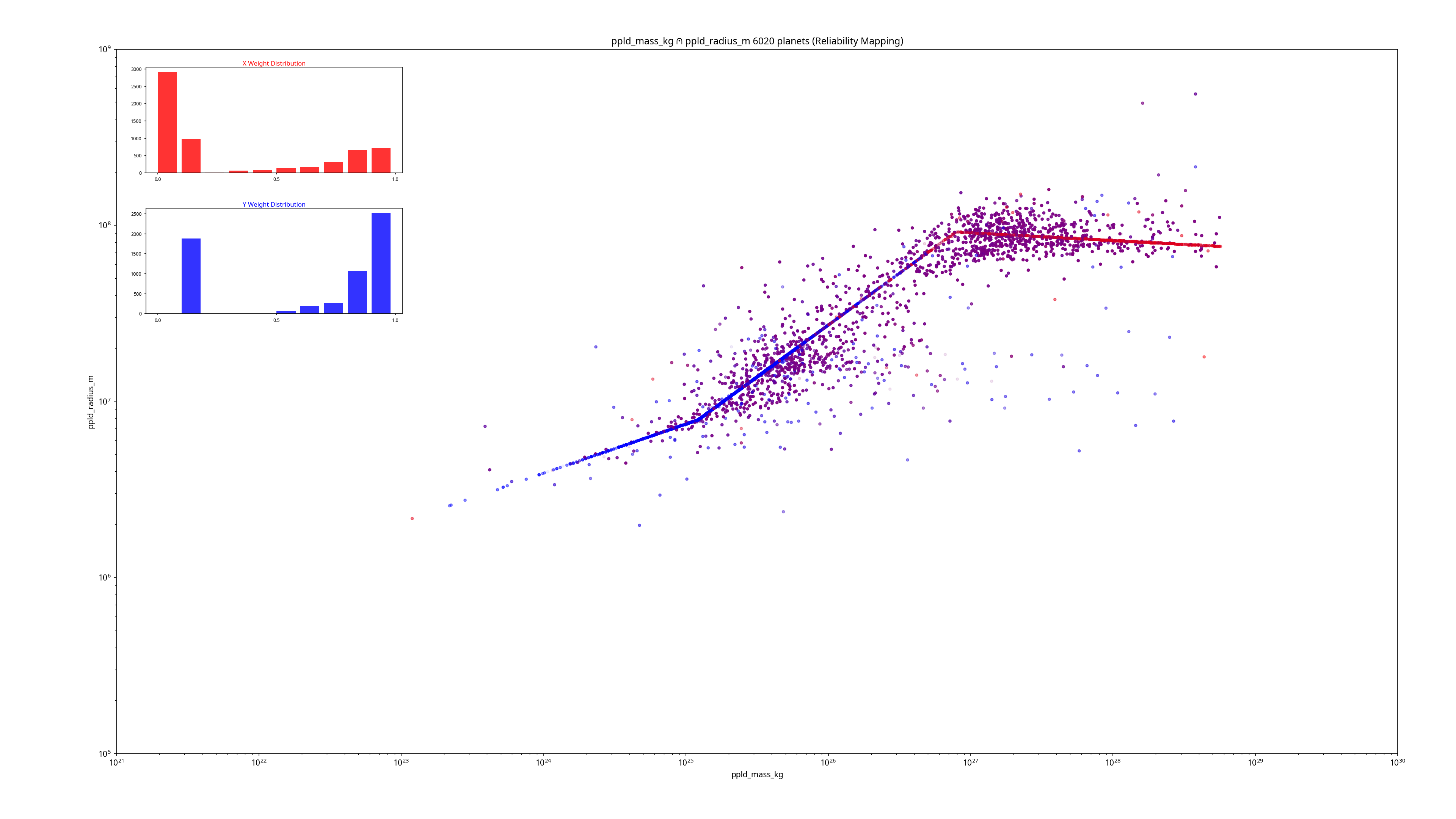 | 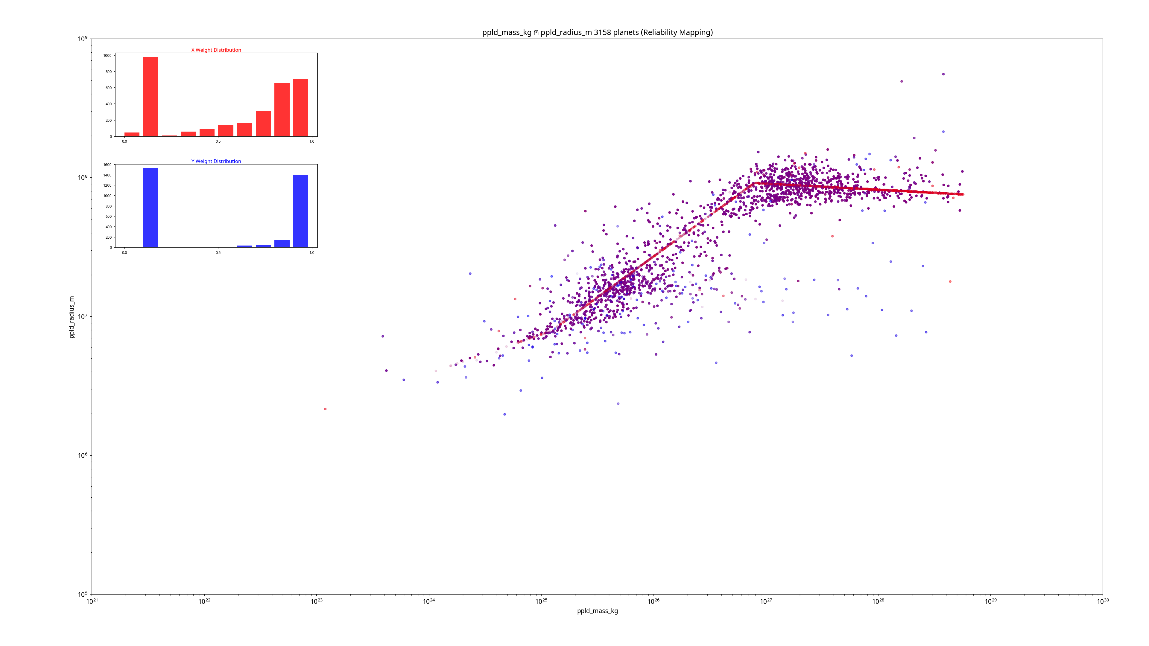 | 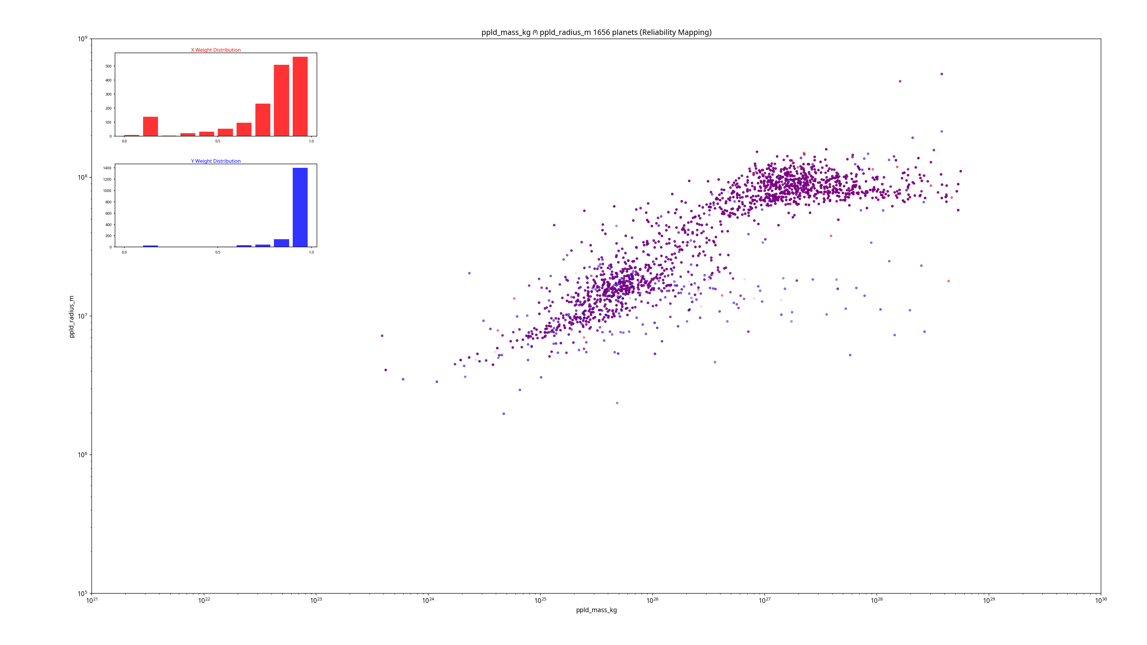 |
Figure 2. Mass vs. Density
| Unfiltered, showing Chen & Kipping piecewise power law artefact | Filtered | Filtered More |
|---|---|---|
| 6,020 records | 3,158 records | 1,656 |
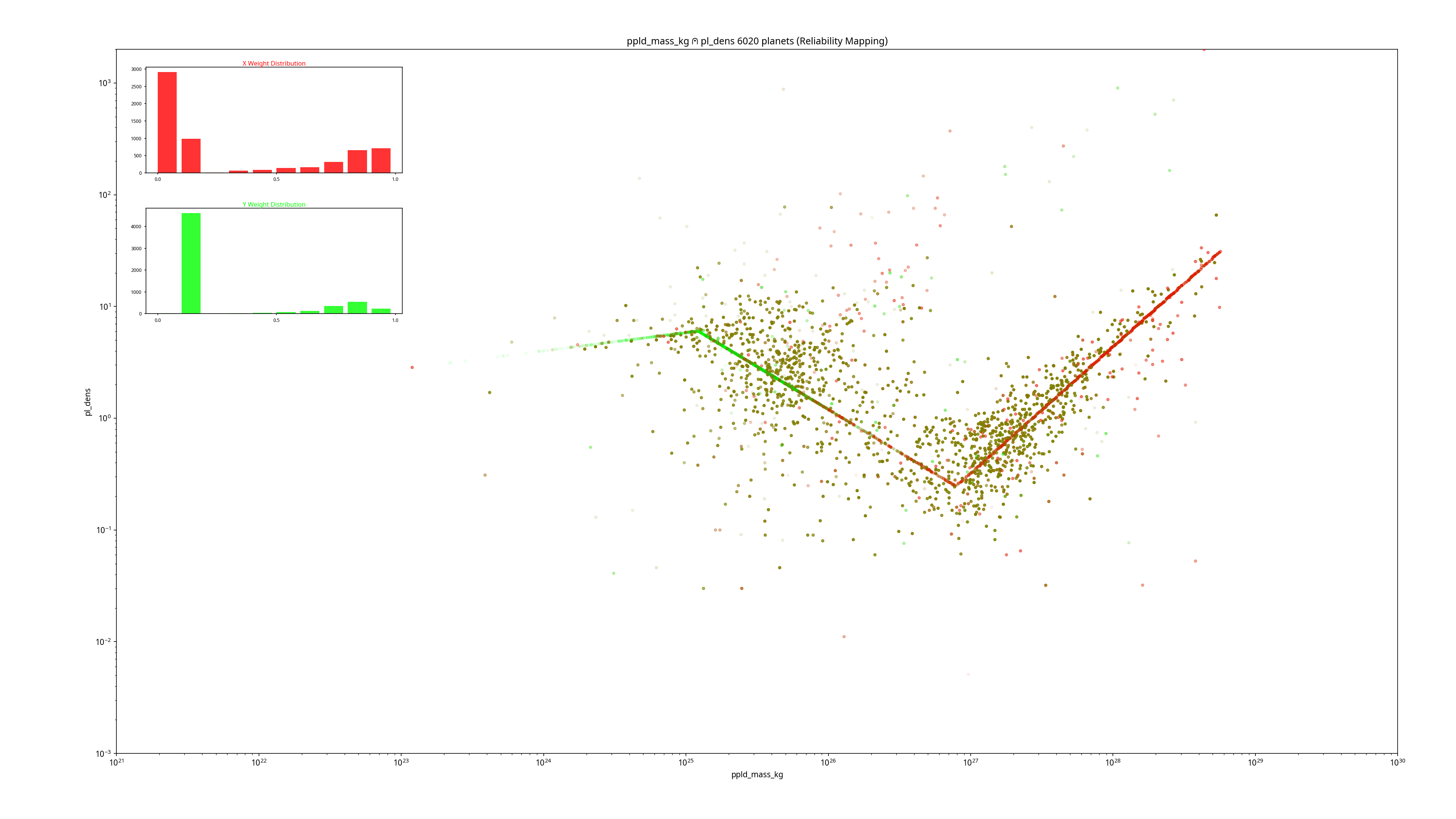 | 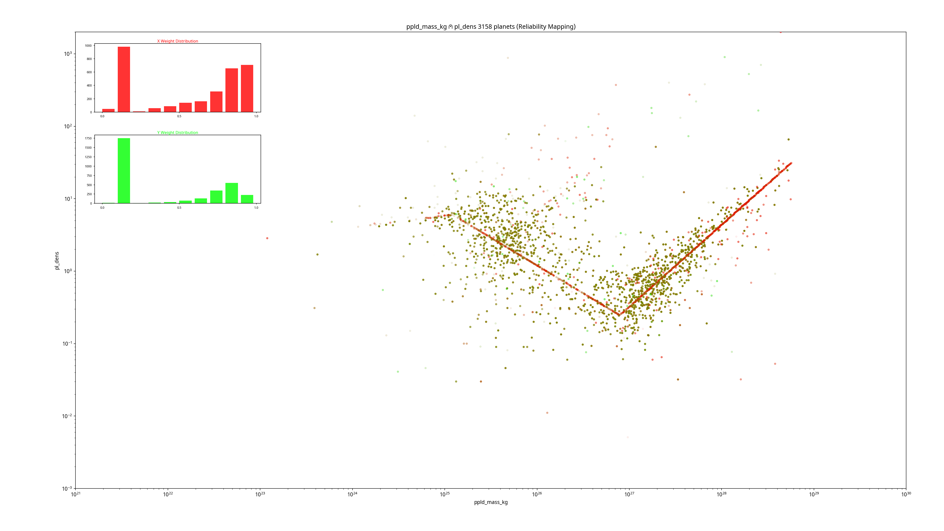 | 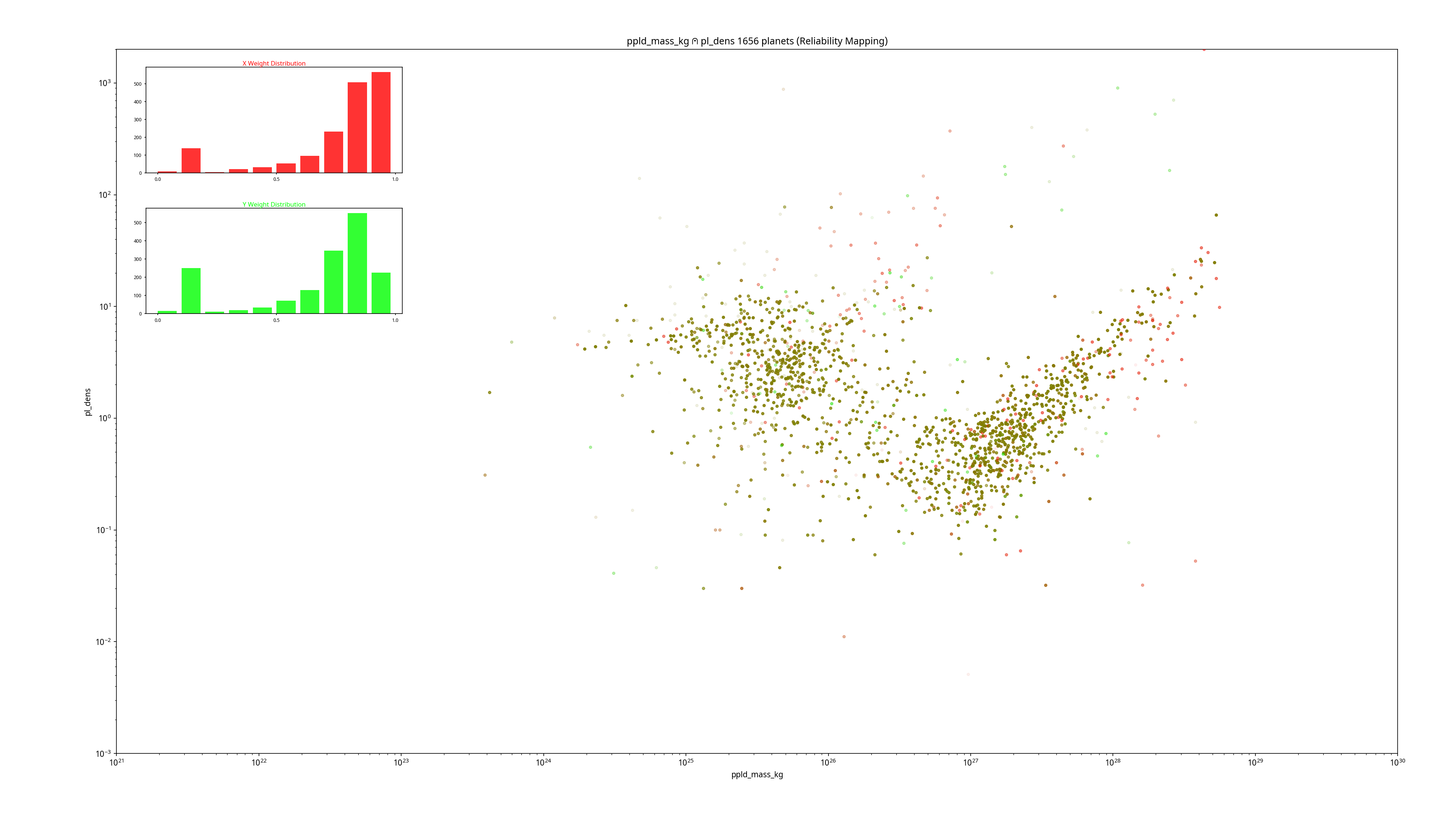 |
Figure 3. Graph log₁₀(mass slice) vs. b (power-law exponent)
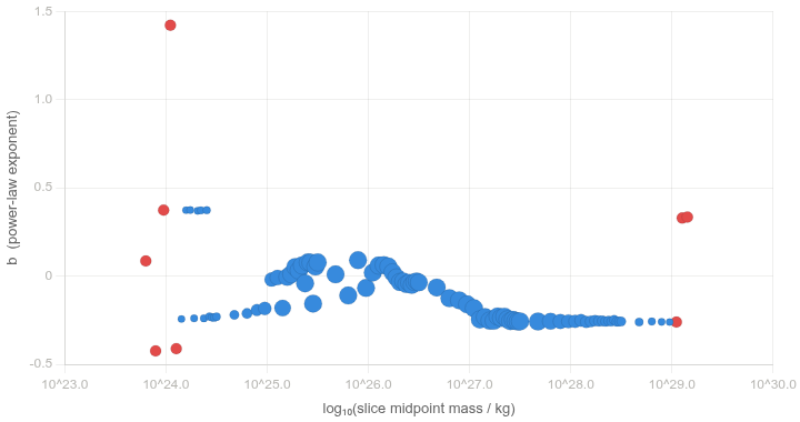
The chart shows some clear patterns worth noting: The red cluster (sparse slices, n < 20) in the 10²³–10²⁴ range is very noisy — b swings from -0.42 to +1.42, which makes sense given only 6–17 data points going into the MCMC. Don't trust those. The blue points tell a more interesting story — there appear to be at least two regimes:
- Around 10²⁴–10²⁶ kg, b is scattered near 0 with high b_std, suggesting the sampler is struggling to find a consistent slope — this is likely the transition zone between Durand-Manterola's Class A/B boundary (~5×10²⁵ kg)
- From ~10²⁶ kg upward, b converges tightly around -0.257 with very small b_std — that's a strong, stable signal in the Jovian/Class C regime
The fact that b is negative in the upper mass range is physically interesting — it means radius shrinks slightly with increasing mass for gas giants, which is consistent with electron degeneracy pressure effects in the Jovian regime. Durand-Manterola's Class C exponent from the paper would be the direct comparison point as wider slices are run.
Figure 4. Potential Class A-B transition?

The disruption is very visible. A few things worth noting:
The boundary signal is real. b is tracking smoothly around -0.19 right up to 3×10²⁵, then it collapses toward zero and briefly goes positive at 4×10²⁵, before snapping back to ~-0.20 at 4.5×10²⁵. That's the MCMC telling you the power law genuinely breaks at that point — you're fitting across two populations with different exponents and the sampler can't settle.
The D-M ambiguity (3 vs 5 ×10²⁵) might actually be a real physical feature, not a typo. The disruption starts at ~3×10²⁵ and doesn't resolve until ~4.5×10²⁵. So the "boundary" may not be a sharp line — it could be a transition zone ~1.5 decades wide, and Durand-Manterola may have been reporting different edges of it in different places in the paper.
The oscillating bimodal pattern in the 10²⁴–3×10²⁵ region (alternating between b≈+0.37 and b≈-0.25) is suspicious — that's almost certainly the sampler flipping between two local modes in the posterior rather than a real physical signal. Those slices have very few points and the GMM mixture prior is probably letting the chain wander between two interpretations of the data.
Future directions and things to consider
Refit the power laws on the modern dataset. With thousands of planets now available, the Durand-Manterola exponents could be refitted and compared to the 2011 values. This would test whether the classification scheme holds at scale. Segemented Regression, the Chow test, and Recursive Residuals
Use better fitting methods. Ordinary least squares in log space assumes symmetric, equal-weight Gaussian errors on logged quantities — a poor match to real exoplanet data. More appropriate methods include:
- Weighted least squares — weights each point by 1/σ², respecting measurement quality
- Orthogonal distance regression (ODR) — accounts for uncertainties on both axes (
scipy.odr) - Bayesian regression with intrinsic scatter — implemented: the
linmixpackage (Kelly 2007) is used for single-slice scatter plot trend lines, and a NumPyro NUTS model (Phan et al. 2019) is used for the sliding-window analysis
Treat class boundaries as uncertain. The hard mass cuts could be replaced with a mixture model or a hierarchical Bayesian model that allows planets near the boundaries to have probabilistic class membership.
Separate calculated from measured densities. Rerunning the analysis on the subset with directly measured densities would test whether the power law structure is robust to the archive's density imputation.
Add escape velocity. Durand-Manterola's toy model [https://arxiv.org/abs/1111.3986]((Figure 5)) uses escape velocity to explain volatile retention in Class B. This is straightforward to calculate from the same mass and radius data and would add physical context to the dataset.
Add more advanced data filtering. Currently filtering is simplistic. If a row has a field that matches a filter from the command line, that row is discarded. More research needs to be done to see if this simple, indiscrimnate filtering is necessary due to Chen's & Kipping's piecewise power law speading to other columns, or if more sophistacted filtered (i.e. boolean logic) could increase the size of the comparison sets.
Citation
If you use this dataset or script in your work, please cite the NASA Exoplanet Archive:
NASA Exoplanet Archive. Planetary Systems Composite Parameters Table. DOI: 10.26133/NEA12
For the Durand-Manterola classification:
Durand-Manterola, H.J. (2011). Planets: Power Laws and Classification. DOI arXiv:1111.3986
For the mass-radius relation used by the archive to fill missing radii/masses:
Chen, J., & Kipping, D. (2017). Probabilistic Forecasting of the Masses and Radii of Other Worlds. ApJ, 834, 17. DOI: 10.3847/1538-4357/834/1/17
For statistical methods
Kelly, Brandon C. (2007) Some Aspects of Measurement Error in Linear Regression of Astronomical Data DOI: 10.1086/519947
Phan, D., Pradhan, N., & Jankowiak, M. (2019). Composable Effects for Flexible and Accelerated Probabilistic Programming in NumPyro. arXiv: 1912.11554
Contributors

18 commits
Similar repos


Languages
Python
96.3%
PowerShell
2.3%
Shell
1.4%
README
Exoplanet Mass–Radius–Density–Gravity Dataset
A Python script that queries the NASA Exoplanet Archive for all confirmed exoplanets with known mass, radius, and density. It then calculates the mass in kilograms and radius in meters, as well as calculates a reliability weighting for each entry, and classifies each planet using the Durand-Manterola (2011) three-class scheme, and exports the result as CSV files. Also creates scatter plots from the data.
Contents
- Quickstart
- Methodology
- Visualization
- Caveats and known limitations
- My Observations
- Future directions
- Citation
Quickstart
Requirements: Python 3.10+, git
Automated install (Linux/macOS)
curl -fsSL https://raw.githubusercontent.com/CoryAlbrecht/planet-power-law-distribution/main/install.sh | bash
Automated install (Windows)
irm https://raw.githubusercontent.com/CoryAlbrecht/planet-power-law-distribution/main/install.ps1 | iex
Dependencies
Manual install
# Clone repository
$ git clone https://github.com/CoryAlbrecht/planet-power-law-distribution.git
$ cd planet-power-law-distribution

# Create and activate virtual environment
$ python -m venv .venv
$ source .venv/bin/activate  # Linux/macOS
# .\venv\Scripts\Activate.ps1  # Windows

# Install package
$ pip install -e .

# Retrieve data from the NASA Exoplanet Archive database and generate output files
# If the data file is already there and less than a week old, it won't retrieve it again
$ planet-power -r
$ planet-power --retrieve

# Force a data refresh even if the file is less than a week old
$ planet-power -r -R
$ planet-power -r --refresh

# Get the PSCompPars data table instead of the PS data table
$ planet-power -r -p
$ planet-power -r --pscomppars

# Calculate the extra values
$ planet-power --calculate
$ planet-power -c -p

# Join CSV files on the index column and then extract specific columns
$ planet-power --extract -I ./data/pscomppars-raw-data.csv -I ./data/pscomppars-calculated.csv  -f "pl_bmassprov:M-R relationship" -C pl_name -C "~pl_bmassj.*" -C pl_bmassprov -C "~pl_radj.*" -C "~pl_dens.*" -C "~ppld_.*"

# Create a scatter plot graph of the data in a CSV file
planet-power --image --input-file ./data/extracted.filtered-more.csv --x-col-set "ppld_mass_kg" --y-col-set "ppld_radius_m" --output-file ./data/mass-vs-radius-filtered-more.png

# Create a scatter plot graph of the data in a CSV file with a trend line from Bayesian regression
$ planet-power -i -I ./data/extracted.filtered-more.csv -x "ppld_mass_kg" -y "ppld_radius_m" --regression-minimum 1e-30 --regression-maximum 5e+25 -O ./data/mass-vs-radius-filtered-more.png

# Do a slice by slice Bayesian regression analysis of a data set
$ planet-power -a -d 2 -x ppld_mass_kg -y ppld_radius_m -I ./data/extracted.filtered-more.csv
No API key is required. The script queries NASA's public TAP service directly.
CLI Options
| Option | Description | Output |
|---|---|---|
-a, --analyze | Do the Bayesian analyses and print the output, no image | CSV, terminal |
-C COLUMN|~REGEX|@FILE,--column COLUMN|~REGEX|@FILE | Choose columns for fetching or splitting
| |
-c, --calculate | Create extra CSV file with calculated values not in the NASA Exoplanet Archive data | CSV |
-d, --dex-width | 'DEcimal eXponent', the size of a mass slice for Bayesian regression with --analyze | |
-e, --extract | Combine CSV data files and extract specific columns | CSV |
-f COLUMN:REGEX, --filter COLUMN:REGEX | Filter out rows where COLUMN matches REGEX (can be used multiple times) | |
--help-columns | List all available columns in the CSV data files | |
-i, --image | Make a scatter plot graph from a CSV data file | PNG |
-I , --input-file | CSV file to read input data from | |
-m, --regression-minimum | Minimum mass data value for scatter plot regression testing | |
-M, --regression-maximum | Maximum mass data value for scatter plot regression testing | |
-O, --output-file | CSV file to write output data to | |
-r, --retrieve | Fetch data from NASA Exoplanet Archive | CSV |
-R, --refresh | Force refresh of raw data from NASA Exoplanet Archive, requires -r / --retrieve | |
-p, --pscomppars | Use the "PsCompPars" data table from the NASA Exoplanet Archive | |
-t TAG, --tag TAG | Tag to append to split output filenames | |
-x, --x-col-set | Select a group of columns to use as the X-axis data with -i, --image | |
-y, --y-col-set | Select a group of columns to use as the y-axis data with -i, --image |
All output data ends up in the ./data directory.
Methodology
Data source
The script utilizes the NASA Exoplanet Archive TAP service to retrieve either the ps (Planetary Systems) or pscomppars (Planetary Systems Composite Parameters) table. The pscomppars table is preferred for population studies as it provides a single, representative set of parameters for each confirmed planet. Data is cached locally for up to one week; use --refresh to force a new download.
Solar system reference objects
constants.py embeds a curated table of 37 solar system bodies (planets, major moons, and dwarf planets) with mass, radius, density, and reliability weights sourced from spacecraft missions and published ephemerides. This data is available for overlay or comparison in future visualizations.
Weighting
To address the goal of identifying structural breaks without the noise of low-quality data or model-derived values, a normalized weighting system ($0.0$ to $1.0$) is applied to each measurement. The weight is the product of two independent factors, each capturing a different aspect of data quality.
1. Provenance factor ($W_{prov}$)
For mass, the archive's pl_bmassprov column records how the best-mass estimate was obtained. The provenance factor penalises measurement types that are less reliable for population-level power-law fitting:
| Provenance | $W_{prov}$ | Notes |
|---|---|---|
Mass | 1.0 | True mass from inclination-resolved orbit |
Msin(i)/sin(i) | 1.0 | Inclination known; true mass recovered |
Msini | 0.2 | Lower bound only; inclination unknown |
M-R relationship | 0.0 | Fully model-derived via Chen & Kipping (2017) |
| Unknown / missing | 0.1 | Conservative fallback |
Radius and density do not have an equivalent provenance column in the archive, so their provenance factor defaults to $1.0$ and the weight is determined entirely by the precision factor and error completeness below.
2. Error completeness penalty
If both error bars are present, no additional penalty is applied. If only one error bar exists, $W_{prov}$ is multiplied by $0.6$ before the precision factor is calculated — separating the question of whether the uncertainty is fully characterised from how large it is. If neither error bar is present, the function returns $W_{prov} × 0.1$ immediately as a heavy penalty.
3. Precision factor ($W_{prec}$)
An exponential decay is applied to the relative uncertainty $\delta = \sigma / v$, where $\sigma$ is the mean of the available absolute error bars and $v$ is the measured value:
$$W_{prec} = e^{-\delta}$$
This ensures that points with high relative uncertainty fade naturally while those with small errors relative to their value retain a weight close to $1.0$. Note that $\sigma$ is calculated as the mean of whichever error bars exist — the completeness penalty above handles the asymmetry separately rather than folding it into $\sigma$.
Combined weight
$$W = \mathrm{clip}(W_{prov} \cdot W_{prec},\ 0,\ 1)$$
This weighting scheme combines provenance quality with measurement precision using exponential decay of relative uncertainty. It shares the same $[0, 1]$ range as inverse-variance weighting and can be passed directly to fitting routines such as linmix or scipy.odr. The exponential form is deliberately gentler than $1/\sigma^2$ at large uncertainties, treating poorly-measured planets as low-confidence rather than discarding them.
Bayesian power-law regression
The --analyze command runs a sliding-window Bayesian regression across mass slices to estimate the local power-law exponent $b$ in $R = a \cdot M^b$ at each point along the mass axis.
Primary sampler — NumPyro NUTS (run_numpyro_slice_weighted):
The production analysis uses JAX/NumPyro with the No-U-Turn Sampler (NUTS). The probabilistic model includes:
- A $K=2$ Gaussian mixture prior on the latent true log₁₀(mass), capturing the bimodal terrestrial/Jovian population structure without forcing a unimodal prior.
- Per-point heteroscedastic measurement noise on both axes (weight-scaled asymmetric errors propagated into log₁₀ space).
- A HalfNormal prior on intrinsic scatter in log₁₀(radius) beyond measurement noise.
- 500 warm-up steps and 1 000 posterior samples per slice via a single chain.
Each slice is run in a separate spawned worker process (up to 8 in parallel) so the JAX/XLA runtime is isolated from the main process and slices never contend for GPU memory. Results are streamed to CSV in real time as workers complete.
Secondary sampler — linmix Gibbs (run_bayesian_slice_weighted):
A linmix-based Gibbs sampler (Kelly 2007) is retained for single-slice regression with an optional mass range, used when generating a trend line for the --image scatter plot. It mirrors the same data-preparation pipeline (weight-scaled errors, log₁₀ propagation, $K=2$ GMM on $x$) but uses a Gibbs sampler rather than NUTS.
Both functions symmetrize asymmetric error bars (averaging $|\sigma^+|$ and $|\sigma^-|$) and scale the resulting linear error by $1/\sqrt{w}$ before propagating into log₁₀ space, so that lower-reliability measurements contribute wider error bars to the fit rather than being discarded.
Surface gravity
Surface gravity ($g$) is calculated using the standard Newtonian formula: $$g = \frac{G \cdot M}{R^2}$$ where $M$ is the caclulated mass in kg and $R$ is the calculated radius in meters.
Durand-Manterola classification
Planets are categorized into three classes based on their mass ($M$):
- Class A: $M < 5 \times 10^{25}$ kg (Earth-like/Super-Earths)
- Class B: $5 \times 10^{25} \text{ kg} \le M < 1 \times 10^{27}$ kg (Neptune-like/Sub-Saturns)
- Class C: $M \ge 1 \times 10^{27}$ kg (Gas Giants/Brown Dwarfs)
Visualization
The script generates high-resolution scatter plots (e.g., Mass vs. Radius) using a Reliability Color Space to visually represent the $\u2A40$ intersection of data confidence:
- Dual-Gradient Error Crosses: * Horizontal Bars: Transition from White ($0.0$) to Red ($1.0$) based on the $x$-axis weighting.
- Vertical Bars: Transition from White ($0.0$) to Blue ($1.0$) based on the $y$-axis weighting.
- Scatter Points:
- The central dots use additive mixing: Red (X-weight) + Blue (Y-weight) = Purple.
- The opacity (alpha) of the dot is the arithmetic mean of the two weights.
- Weight Distribution Insets: Small bar charts in the upper-left display decile distributions for both weightings, allowing for immediate assessment of dataset quality and the prevalence of model-contaminated points.
Caveats and known limitations
PSCompPars is not self-consistent. Parameters for a single planet may be drawn from different publications. This is appropriate for demographic studies but should be treated with caution for any individual planet.
Density may be calculated, not measured. Many densities in the archive are derived from mass and radius rather than independently measured. If your analysis requires only directly measured densities, filter on pl_dens_reflink NOT LIKE '%alculated%' (retrievable by adding pl_dens_reflink to the query).
Radius is a transit radius. It is not a volumetric mean or equatorial radius in the Solar System sense. For gas giants, it is pressure-level and wavelength-dependent. The Jupiter and Earth reference radii used for unit conversion are equatorial values, introducing a small systematic inconsistency.
DM class boundaries were chosen by eye. The paper gives no formal method for determining the A/B and B/C boundaries. The text states that planets in different mass ranges "seem to follow" different power laws — the cuts were placed where the slope of the point cloud appeared to change on the log-log plot, with no statistical breakpoint test and no uncertainty on the boundary locations themselves. The correlation coefficients in Table 1 validate the fits given the chosen boundaries, but do not independently justify where the boundaries sit. With a modern dataset of thousands of planets, a more rigorous approach would be to treat the boundary locations as free parameters — for example using piecewise regression breakpoint detection (pwlf) or a hierarchical Bayesian model — rather than inheriting the 2011 visual judgement. Planets near the boundaries (especially in the B/C transition region around 10²⁷ kg) may be ambiguously classified under the current hard cuts.
DM power laws were fitted with OLS in log space. This minimises relative errors and weights all planets equally regardless of measurement quality. It is not equivalent to fitting in linear space, and the resulting coefficients can be sensitive to outliers. Several of the correlation coefficients in the original paper — particularly for surface gravity in Class B (R = 0.248) and radius in Class C (R = 0.120) — fall below or near the paper's own critical significance threshold, so those specific power laws should be interpreted cautiously.
The 2011 dataset was small. The paper used 92 transiting exoplanets; the current NASA archive contains several thousand confirmed planets with measured radii. The class structure and power law exponents may shift with the larger, more diverse modern sample.
My Observations
Three distinct groups of planets that can be seen in the unfiltered data with a very strong central line with two knees in it.
- A <= 1.2×10^25
- 1.2×10^25 <= B <= 8.1×10^26
- C >= 8.1×10^26
But the inflection points between the groups are oddly sharp. When a planet has a measured mass but no observed transit radius, the NASA Exoplanet Archive calculates the mass or radius when missing using the Chen & Kipping (2017) piecewise power law. That relation has hard breakpoints built into it — the Archive's own documentation lists the exact boundaries at 2.04, 132, and 26,600 M_Earth, or 1.22×10^25 kg, 7.90×10^26 kg, and 1.589×10^29 kg.
The Exoplanet Archive data has the pl_bmassprov column, which means exoplanet mass can be filtered and weight a bit more granularly by mass to help get rid of the Chen & Kipping artefact. While that does work somewhat, making the central line described above a bit weaker, especially for lower mass planets, we still need to filter out the ones where radius is calculated rather than observed.
The three groups exist after such weighting and filtering, but are much more fuzzy and closer to Durand-Manterola's originals ranges. Closer analysis needs to be done to see if Durand-Manterola's power law curves are still accurate with the expanded dataset, or if they need to be adjusted.
Figure 1. Mass vs. Radius
| Unfiltered, showing Chen & Kipping piecewise power law artefact | Filtered | Filtered More |
|---|---|---|
| 6,020 records | 3,158 records | 1,656 |
| | |
Figure 2. Mass vs. Density
| Unfiltered, showing Chen & Kipping piecewise power law artefact | Filtered | Filtered More |
|---|---|---|
| 6,020 records | 3,158 records | 1,656 |
| | |
Figure 3. Graph log₁₀(mass slice) vs. b (power-law exponent)
The chart shows some clear patterns worth noting: The red cluster (sparse slices, n < 20) in the 10²³–10²⁴ range is very noisy — b swings from -0.42 to +1.42, which makes sense given only 6–17 data points going into the MCMC. Don't trust those. The blue points tell a more interesting story — there appear to be at least two regimes:
- Around 10²⁴–10²⁶ kg, b is scattered near 0 with high b_std, suggesting the sampler is struggling to find a consistent slope — this is likely the transition zone between Durand-Manterola's Class A/B boundary (~5×10²⁵ kg)
- From ~10²⁶ kg upward, b converges tightly around -0.257 with very small b_std — that's a strong, stable signal in the Jovian/Class C regime
The fact that b is negative in the upper mass range is physically interesting — it means radius shrinks slightly with increasing mass for gas giants, which is consistent with electron degeneracy pressure effects in the Jovian regime. Durand-Manterola's Class C exponent from the paper would be the direct comparison point as wider slices are run.
Figure 4. Potential Class A-B transition?
The disruption is very visible. A few things worth noting:
The boundary signal is real. b is tracking smoothly around -0.19 right up to 3×10²⁵, then it collapses toward zero and briefly goes positive at 4×10²⁵, before snapping back to ~-0.20 at 4.5×10²⁵. That's the MCMC telling you the power law genuinely breaks at that point — you're fitting across two populations with different exponents and the sampler can't settle.
The D-M ambiguity (3 vs 5 ×10²⁵) might actually be a real physical feature, not a typo. The disruption starts at ~3×10²⁵ and doesn't resolve until ~4.5×10²⁵. So the "boundary" may not be a sharp line — it could be a transition zone ~1.5 decades wide, and Durand-Manterola may have been reporting different edges of it in different places in the paper.
The oscillating bimodal pattern in the 10²⁴–3×10²⁵ region (alternating between b≈+0.37 and b≈-0.25) is suspicious — that's almost certainly the sampler flipping between two local modes in the posterior rather than a real physical signal. Those slices have very few points and the GMM mixture prior is probably letting the chain wander between two interpretations of the data.
Future directions and things to consider
Refit the power laws on the modern dataset. With thousands of planets now available, the Durand-Manterola exponents could be refitted and compared to the 2011 values. This would test whether the classification scheme holds at scale. Segemented Regression, the Chow test, and Recursive Residuals
Use better fitting methods. Ordinary least squares in log space assumes symmetric, equal-weight Gaussian errors on logged quantities — a poor match to real exoplanet data. More appropriate methods include:
- Weighted least squares — weights each point by 1/σ², respecting measurement quality
- Orthogonal distance regression (ODR) — accounts for uncertainties on both axes (
scipy.odr) - Bayesian regression with intrinsic scatter — implemented: the
linmixpackage (Kelly 2007) is used for single-slice scatter plot trend lines, and a NumPyro NUTS model (Phan et al. 2019) is used for the sliding-window analysis
Treat class boundaries as uncertain. The hard mass cuts could be replaced with a mixture model or a hierarchical Bayesian model that allows planets near the boundaries to have probabilistic class membership.
Separate calculated from measured densities. Rerunning the analysis on the subset with directly measured densities would test whether the power law structure is robust to the archive's density imputation.
Add escape velocity. Durand-Manterola's toy model [https://arxiv.org/abs/1111.3986]((Figure 5)) uses escape velocity to explain volatile retention in Class B. This is straightforward to calculate from the same mass and radius data and would add physical context to the dataset.
Add more advanced data filtering. Currently filtering is simplistic. If a row has a field that matches a filter from the command line, that row is discarded. More research needs to be done to see if this simple, indiscrimnate filtering is necessary due to Chen's & Kipping's piecewise power law speading to other columns, or if more sophistacted filtered (i.e. boolean logic) could increase the size of the comparison sets.
Citation
If you use this dataset or script in your work, please cite the NASA Exoplanet Archive:
NASA Exoplanet Archive. Planetary Systems Composite Parameters Table. DOI: 10.26133/NEA12
For the Durand-Manterola classification:
Durand-Manterola, H.J. (2011). Planets: Power Laws and Classification. DOI arXiv:1111.3986
For the mass-radius relation used by the archive to fill missing radii/masses:
Chen, J., & Kipping, D. (2017). Probabilistic Forecasting of the Masses and Radii of Other Worlds. ApJ, 834, 17. DOI: 10.3847/1538-4357/834/1/17
For statistical methods
Kelly, Brandon C. (2007) Some Aspects of Measurement Error in Linear Regression of Astronomical Data DOI: 10.1086/519947
Phan, D., Pradhan, N., & Jankowiak, M. (2019). Composable Effects for Flexible and Accelerated Probabilistic Programming in NumPyro. arXiv: 1912.11554
Similar repos
Contributors
18 commits
Languages
Python
96.3%
PowerShell
2.3%
Shell
1.4%