
README
monohunter
Find single long-period mono-transits in public TESS light curves — the single-transit events that periodic pipelines (SPOC/QLP, which fold on a period) structurally under-find. Built so many people can each search under-covered targets and combine machine-readable finds.


New here? Run it in your browser — no install. The quickstart notebook installs monohunter in Colab, recovers a known single transit to prove it works, then scans any star you pick. Open it with the badge above.
Why
Automated TESS pipelines run periodic searches (BLS/TLS) over every target. A single transit has no period to fold on, so those searches miss it. Real long-period planets have been co-discovered exactly here (e.g. TOI-2180 b, found from one ~24-hour transit). monohunter targets that gap.
Install
pip install monohunter
Python 3.10+. Pulls in lightkurve, wotan, astroquery, scipy, matplotlib. The
ASAS-SN ground cross-check needs one extra: pip install monohunter[ground].
Or run it with Docker (no Python setup)
docker run --rm -v monohunter-data:/data ghcr.io/rinkia/monohunter \
    run --tic 298663873 --sectors 19
The container runs as a non-root user, so it persists to a Docker named volume
(monohunter-data above — Docker makes it writable by that user). A plain
-v "$PWD/data:/data" bind mount is root-owned on the host and needs a one-time
chown 10001 data to be writable. For an always-on fresh-data watcher (ideal on a
homelab), docker compose up -d runs monohunter watch-loop on the newest sector in a
resumable, self-healing loop — see docker-compose.yml. To run that
watcher in the cloud, deploy it to Fly.io with the included fly.toml —
see docs/deploy-fly.md.
Usage
Search one target by its TESS Input Catalog (TIC) id:
monohunter run --tic 298663873
This searches every available sector, and for each candidate writes a JSON
find-record + a diagnostic PNG into candidates/. Example (TOI-2180, the
canonical mono-transit — restrict to its sector to keep it quick):
monohunter run --tic 298663873 --sectors 19
# S19: depth=4.09ppt dur=24h SNR=39.4  [known TOI-2180.01] -> candidates/tic298663873_s19.json
Options
| Flag | Default | Meaning |
|---|---|---|
--tic <id> | required | TESS Input Catalog id to search |
--sectors <n...> | all | restrict to specific sector numbers (faster) |
--window <days> | 3.0 | detrend window; must be several × the transit duration or flattening eats the dip |
--outdir <path> | candidates | where JSON + PNG are written |
--no-plot | off | skip PNG generation |
--ffi | off | extract from the Full-Frame Images via TESScut — reaches stars with no pre-made SPOC/QLP light curve |
--dry-run | off | list the sectors available for the TIC and exit (no download/detect) |
Reading a result
Each candidate is one JSON file:
{
  "schema_version": 7,
  "tic": 298663873,
  "sector": 19,
  "cadence_s": 120,
  "event_time_btjd": 1830.77,
  "depth_ppt": 4.09,
  "duration_hr": 23.8,
  "ingress_hr": 2.29,
  "snr": 39.4,
  "tool_version": "0.3.0",
  "known_toi_match": true,
  "known_toi_id": "TOI-2180.01",
  "likely_eb": false,
  "period_constrained": true,
  "p_best_d": 856.0,
  "p_lo_d": 396.0,
  "p_hi_d": 1946.0,
  "next_window_btjd": [3200.0, 3245.0, 3290.0],
  "n_sectors_observed": 1,
  "recurring_dip": false,
  "measured_period_d": null,
  "edge_gap_dist_d": 6.4,
  "baseline_scatter_ppt": 0.21,
  "plot_path": "candidates/tic298663873_s19.png"
}
The two v7 fields are false-positive-triage features computed from the light curve:
edge_gap_dist_d (distance to the nearest sector edge / data gap — FP ramps cluster
there) and baseline_scatter_ppt (per-cadence scatter; faint/noisy stars give
untrustworthy shallow dips). They let the triage model rank survivors on any sector.
| Field | Meaning |
|---|---|
event_time_btjd | dip center, TESS Barycentric Julian Date |
depth_ppt | transit depth (parts per thousand), trapezoid flat-bottom |
duration_hr | total transit duration (first-to-last contact) |
ingress_hr | ingress/egress time from the trapezoid fit (null if uncharacterized) |
snr | detection signal-to-noise; the tool reports candidates at SNR ≥ 7 |
known_toi_match / known_toi_id | whether the target is an existing TESS Object of Interest |
likely_eb | too deep / V-shaped for a planet — flagged as a likely eclipsing binary (labelled, not rejected) |
p_best_d, p_lo_d, p_hi_d | single-transit period estimate + range (see Next-transit ephemeris) |
n_sectors_observed, recurring_dip | multi-sector context: dips in >1 sector flag a periodic/variable star |
measured_period_d | exact period fitted from multiple transit times, when the target recurs across sectors |
Always look at the PNG. SNR alone lies — confirm the marked dip is a real,
centered transit, not a sector-edge ramp, a data gap, or a single bad cadence.
Re-run with a different --window; a real dip survives, an artifact moves or
vanishes. A known_toi_match: false is the interesting case (potentially
unsearched); true still validates the tool.
A candidate is not a discovery. It means a human thinks the dip is real. Confirming a planet needs follow-up (radial velocity, more transits) beyond this tool.
How it works
fetch      search TESS, dedup sectors (prefer 2-min), quality-mask (hard),
           stream one sector at a time
   |
detrend    wotan biweight; window must be >> transit or the dip is flattened away
   |
detect     matched-filter box scan (non-periodic — finds a SINGLE transit),
           red-noise-aware SNR + 7 false-positive guards (edge / gap / scatter /
           momentum-dump ramps)
   |
characterize   trapezoid fit -> true depth, duration, ingress; EB flag
   |
cross-match    flag known TESS Objects of Interest (NASA Exoplanet Archive)
   |
ephemeris      period + next-transit window (single-transit, or exact from
           multiple sectors); multi-sector recurrence flag
   |
FindRecord     versioned + validated JSON  ->  candidates/
The Detector interface is a seam: v1 is the box scan; a GP-based detector
(nuance) can plug in later without touching the pipeline. The versioned
FindRecord JSON is the contract a future aggregation server consumes.
Reuse, not reinvention
Stands on lightkurve, wotan, scipy, and astroquery. monohunter is orchestration + the single-transit gap + result aggregation, not a new detection engine.
Fresh-data watcher (be first)
Institutional pipelines take weeks-to-months to vet a new TESS sector. Run the watcher on a schedule and you process a sector within hours of its release — and a single transit you flag comes with a next-transit window (see below) an observer can still act on.
monohunter watch --sector 90 --max 100 --out watch_out --state watch_state.json
Each run scans the next --max un-processed targets of the sector and prints any
not-yet-known candidates. It's resumable: state tracks which TICs are done,
so scheduled runs continue where the last stopped and a crash loses nothing.
Schedule it to keep chewing through the sector:
# Linux/macOS cron — every 2 hours
0 */2 * * * cd /path/to/monohunter && monohunter watch --sector 90 --max 200

# Windows: Task Scheduler → run the same command on a trigger
Point --sector at the newest released sector. Candidates land in watch_out/;
vet each with monohunter run --tic <id> --sectors <N> to get its PNG, then
submit the good ones (see Contributing).
Reproducible sweeps. watch is the sweep tool — resumable, parallel, and
it logs provenance. For a full sector sweep:
monohunter watch --sector 17 --max 5000 --workers 3 --max-hours 5 \
    --summaries summaries_s17 --csv-log sweeps/sector17.csv
Safety net for long runs. Every network read is capped (a 180 s socket timeout),
watch prints live per-star progress with elapsed/ETA, and --slow-warn S flags any
star taking longer than S seconds — a stall short of the hard timeout is visible
instead of a silent freeze. --max-hours is the wall-clock watchdog: it soft-warns at
80 % of the cap, then force-exits (a hung MAST socket can wedge a worker indefinitely).
It's resumable — re-run to continue where it stopped. Preview a sweep without downloading
anything via monohunter watch --sector N --dry-run (pool size + done/remaining).
--csv-log appends one status row per star (none/novel/error) — the
scan-log a catalog and any retry build from. A star that errors (usually a
transient MAST hiccup) is logged and left un-processed, so simply re-running
the same command retries only the failures — no manual cleanup. --summaries
writes the rotation/variability catalog from the same downloads.
Next-transit ephemeris
When a candidate's target has a catalog stellar density, monohunter estimates the period from the transit duration and predicts when the next transit could occur:
S19: depth=4.09ppt dur=24h SNR=39.4  [known TOI-2180.01]
    P~856d (396-1946d, P_min 15d), next transit ~2027-08-07
Single-transit periods are inherently uncertain (a range, not a precise value) — the output is a targeting window for follow-up, not a confirmed ephemeris. If the stellar density is missing or too uncertain, monohunter reports the period as unconstrained rather than guessing.
Multi-sector sharpens both. A target that dips in more than one sector is
flagged recurring_dip (periodic/variable, not a clean mono-transit), and once
it transits in ≥3 sectors the exact period is fitted from the transit times
(measured_period_d) — vastly tighter than the single-transit range.
Is it observable? observe turns a next-transit window into concrete
"target-up and sky-dark" clock-time intervals for an observer's latitude/longitude —
so you know whether, and when, to point a telescope. Coordinates come from --ra/--dec
or a --tic (fetched from MAST); the window from --start/--end or straight from a
candidate record:
monohunter observe --record contributions/Rinkia/tic400048097_s17.json --lat 45.19 --lon 9.16
#   TIC 400048097 ...: 2026-08-28 21:00 UTC -> 2026-08-29 03:30 UTC  (6.5h)  ...
Tune with --min-alt (default 30°) and --sun-alt (−18° astronomical / −12° nautical).
Astropy only — no extra dependency.
More commands
Anomaly detection — a suite of non-transit light-curve anomaly classes on the same downloads, each reported per sector with a generalized 0–1 anomaly score:
monohunter anomaly --tic 441420236 # AU Mic: flares detected
| Detector | Flags |
|---|---|
| flares | sharp positive brightenings |
| dippers | aperiodic multi-dip young stars (dust) |
| deep dimming | deep (%-level) aperiodic dips — Boyajian / KIC 8462852-like |
| heartbeat | eccentric-binary tidal pulse, once per orbit (phase-localized + bipolar) |
| outbursts | sustained (hours+) brightenings — cataclysmic-variable / nova |
| anomaly score | model-agnostic 0–1 "weirdness" blend, with a component breakdown |
These flags (plus anomaly_score) are also written into the per-star summary catalog
(see below), so a full sweep surfaces the strangest curves for a human to look at.
FFI reach — extract from the Full-Frame Images to search stars with no
pre-made light curve. One target (run --ffi), or a whole cutout at once:
monohunter ffi-batch --tic <center> --sector 14 # every catalog star in one cutout
Ground cross-check — is a candidate's host quiet over years, or a variable star / eclipsing binary? Confirm against ZTF or ASAS-SN:
monohunter ground --tic 198382838 --survey ztf # or --survey asassn
Eclipsing-binary periods — an EB with two or more eclipses in one sector has a
recoverable orbital period. eb finds the eclipse times, splits primary from
secondary by depth, and fits the period from the primary times (their spacing
is exactly one orbit):
monohunter eb --tic 271763138 --sectors 15
# S15: 2 eclipses (1 primary) (primary+secondary) -> period needs >=2 same-type eclipses
A lone primary+secondary pair is left unrecoverable on purpose — on an eccentric orbit the secondary sits at an unknown phase, so the primary-secondary gap is not a period fraction. The tool never reports a confident wrong period.
Rotation / variability catalog — the same download that feeds the transit scan
also yields a per-star rotation period, variability amplitude, flare count, and a
sub-class. summarize writes one JSON per star; catalog aggregates them:
monohunter summarize --tic 100010286              # rotation/variability/flares/dipper + subclass
monohunter catalog --summaries summaries --out catalog.csv
The subclass field splits variables into eclipsing (≥2 eclipse-shaped dips),
rotator (non-sinusoidal spot modulation), and physical pulsator classes —
rr_lyrae (large-amplitude sawtooth), delta_scuti (fast, < 0.3 d), gamma_dor
(slow g-mode, 0.3–3 d) — via periodogram harmonics + fold shape. Each catalog row also
carries the anomaly flags (anomaly_score, is_deep_dipper, n_outbursts,
is_heartbeat) from the same download.
Write one line per star to a single file with a .jsonl --summaries / --outdir
target — one open instead of thousands of tiny JSONs when building a big catalog.
Repopulate an existing catalog (e.g. to backfill new fields) by re-summarizing every
star it lists, in parallel and resumably:
monohunter summarize --from-catalog catalogs/sector18.csv --outdir summaries_s18 \
    --workers 4 --max-hours 6      # progress per star; watchdog + --slow-warn as in watch
Rotation-period distribution — a population science figure straight from a catalog CSV: the period distribution and the period–amplitude relation over every rotator in the sweep:
monohunter rotation-plot --csv catalogs/sector15.csv --sector 15 --out rotation.png
Faster sweeps — watch (and the sweep scripts) take --workers N for
parallel MAST downloads (network-bound; keep it modest, 4-8).
Crowd vetting + triage — turn a pile of candidates into a labelled queue, then rank future survivors by how much they deserve a human's eyes:
monohunter vet --candidates candidates --out _vet      # static page: PNGs + label buttons
monohunter triage-train --labels labels/seed_labels.csv --sweeps sweeps
monohunter triage --candidates candidates --top 10     # ranks by P(worth vetting)
The vetting page exports labels as JSON; those labels train the triage model,
which then puts the real finds at the top of the next sweep's queue. --top N
(and --min-prob P) trims the ranked output to the short-list worth a human's time.
Novelty cross-match — is a find already a known variable star? Cone-matches against both the AAVSO Variable Star Index (VSX) and Gaia DR3 variability; a candidate is "novel" only when unknown to both:
monohunter novelty --tic 298009554 # or --candidates <dir> to batch
FFI star pool — enumerate the non-SPOC stars in a sky region (catalog stars with no 2-min light curve) and sweep them via the FFI path — a true FFI sweep:
monohunter ffi-pool --tic <center> --sector 18 --radius 0.2 --out ffi_pool.txt
monohunter watch --sector 18 --ffi --target-pool ffi_pool.txt
Cache hygiene — a truncated MAST download leaves a corrupt partial FITS that can wedge
a later run; sweep them (exact-size stubs) with monohunter clean-cache (--dry-run to
preview).
Survey sensitivity (completeness)
A find list without a sensitivity function is a hobby list; with one it is a survey.
completeness injects synthetic box transits across a depth × duration grid into real
light curves and runs the full detect pipeline on each, measuring the recovered
fraction — what the survey would have caught, and what it would have missed.
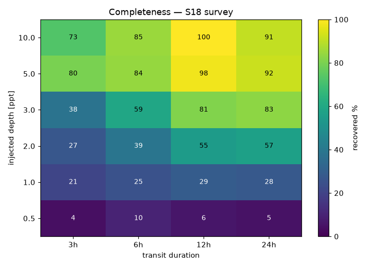
Sector 18, mean over 10 quiet stars: ~50% complete at 2–3 ppt for long (12–24 h) transits and ~90% by 5 ppt, while sub-1 ppt dips are largely missed. Reproduce (or plot your own sector) with:
monohunter completeness --sample 10 --catalog catalogs/sector18.csv --sector 18 \
  --n 10 --plot completeness_s18.png
Community leaderboard (swarm)
Submitted candidates are aggregated into one ranked list — deduped by
(tic, sector), ranked by novelty (not a known TOI), cross-submitter agreement,
and SNR. Live at https://rinkia.github.io/monohunter/, rebuilt automatically
on every merged contribution.
Vetted candidates worth follow-up (RV, characterization, a second transit) are tracked in docs/followup-targets.md — currently led by TIC 400048097, a bright, uncatalogued star with one clean 2.5% transit.
Confirmation tracking (followup)
A candidate is not a discovery until it's confirmed. followup tracks that lifecycle —
pending → observing → confirmed | rejected — as git-friendly per-target JSON records in
followups/, so the community can see what's pending, being observed,
confirmed, or ruled out. It's the outcome side of observe: observe says when to point,
followup records what happened.
monohunter followup add --tic 400048097 --sector 17 \
    --from-record contributions/Rinkia/tic400048097_s17.json --status observing --note "watching next window"
monohunter followup set --tic 400048097 --sector 17 --status confirmed --note "2nd transit caught 2026-08-29"
monohunter followup list --status observing
add seeds the TIC, sector, and next-transit window from a candidate record; set
applies a validated status transition with a dated note and observer; list shows the
ledger. The three live targets ship pre-seeded. Extend it by PR, like contributions/.
Build it yourself from a contributions/ tree:
monohunter aggregate --contributions contributions --out _site
# writes _site/index.html + _site/leaderboard.json
This is phase 1 of the swarm: pure aggregation over the PR flow, no backend. A live coordination server (handing out targets so no two people search the same star) is a later increment, worth building only once there's real contention.
One-time to publish: repo Settings → Pages → Source = "GitHub Actions"
(the pages.yml workflow does the rest).
Contributing
Found a candidate, or want to improve the detector? See CONTRIBUTING.md.
- No git? Use the issue form. Open a Submit a candidate issue — fill in the TIC, sector, stats, drag in the PNG, tick the vetting boxes. A maintainer turns a complete submission into a leaderboard entry.
- Comfortable with git? Candidate submissions go to
contributions/<username>/via the candidate PR template.
Development
git clone https://github.com/Rinkia/monohunter
cd monohunter
python -m venv .venv && . .venv/Scripts/activate   # Windows
pip install -e ".[dev]"
pytest -q                 # fast, offline unit tests
pytest --runslow          # + live real-data regression (hits MAST)
Releasing to PyPI
CI (.github/workflows/ci.yml) runs the tests on every push. Publishing
(.github/workflows/release.yml) fires on a version tag and uses Trusted
Publishing — no token in GitHub.
One-time PyPI setup (before the first release):
- On PyPI: Account → Publishing → Add a pending publisher:
- PyPI project name:
monohunter - Owner:
Rinkia· Repository:monohunter - Workflow:
release.yml· Environment: leave blank (Any)
- PyPI project name:
- (Optional) For a manual approval gate, create a GitHub Environment, set it
as the pending-publisher Environment, and add
environment: <name>back to thepublishjob inrelease.yml.
Then release:
# bump version in pyproject.toml + monohunter/__init__.py, update CHANGELOG.md
git tag vX.Y.Z
git push origin vX.Y.Z
License
MIT.
Contributors

110 commits
See what people are saying
Similar repos


Languages
Jupyter Notebook
90.7%
Python
9.2%
README
monohunter
Find single long-period mono-transits in public TESS light curves — the single-transit events that periodic pipelines (SPOC/QLP, which fold on a period) structurally under-find. Built so many people can each search under-covered targets and combine machine-readable finds.
New here? Run it in your browser — no install. The quickstart notebook installs monohunter in Colab, recovers a known single transit to prove it works, then scans any star you pick. Open it with the badge above.
Why
Automated TESS pipelines run periodic searches (BLS/TLS) over every target. A single transit has no period to fold on, so those searches miss it. Real long-period planets have been co-discovered exactly here (e.g. TOI-2180 b, found from one ~24-hour transit). monohunter targets that gap.
Install
pip install monohunter
Python 3.10+. Pulls in lightkurve, wotan, astroquery, scipy, matplotlib. The
ASAS-SN ground cross-check needs one extra: pip install monohunter[ground].
Or run it with Docker (no Python setup)
docker run --rm -v monohunter-data:/data ghcr.io/rinkia/monohunter \
    run --tic 298663873 --sectors 19
The container runs as a non-root user, so it persists to a Docker named volume
(monohunter-data above — Docker makes it writable by that user). A plain
-v "$PWD/data:/data" bind mount is root-owned on the host and needs a one-time
chown 10001 data to be writable. For an always-on fresh-data watcher (ideal on a
homelab), docker compose up -d runs monohunter watch-loop on the newest sector in a
resumable, self-healing loop — see docker-compose.yml. To run that
watcher in the cloud, deploy it to Fly.io with the included fly.toml —
see docs/deploy-fly.md.
Usage
Search one target by its TESS Input Catalog (TIC) id:
monohunter run --tic 298663873
This searches every available sector, and for each candidate writes a JSON
find-record + a diagnostic PNG into candidates/. Example (TOI-2180, the
canonical mono-transit — restrict to its sector to keep it quick):
monohunter run --tic 298663873 --sectors 19
# S19: depth=4.09ppt dur=24h SNR=39.4  [known TOI-2180.01] -> candidates/tic298663873_s19.json
Options
| Flag | Default | Meaning |
|---|---|---|
--tic <id> | required | TESS Input Catalog id to search |
--sectors <n...> | all | restrict to specific sector numbers (faster) |
--window <days> | 3.0 | detrend window; must be several × the transit duration or flattening eats the dip |
--outdir <path> | candidates | where JSON + PNG are written |
--no-plot | off | skip PNG generation |
--ffi | off | extract from the Full-Frame Images via TESScut — reaches stars with no pre-made SPOC/QLP light curve |
--dry-run | off | list the sectors available for the TIC and exit (no download/detect) |
Reading a result
Each candidate is one JSON file:
{
  "schema_version": 7,
  "tic": 298663873,
  "sector": 19,
  "cadence_s": 120,
  "event_time_btjd": 1830.77,
  "depth_ppt": 4.09,
  "duration_hr": 23.8,
  "ingress_hr": 2.29,
  "snr": 39.4,
  "tool_version": "0.3.0",
  "known_toi_match": true,
  "known_toi_id": "TOI-2180.01",
  "likely_eb": false,
  "period_constrained": true,
  "p_best_d": 856.0,
  "p_lo_d": 396.0,
  "p_hi_d": 1946.0,
  "next_window_btjd": [3200.0, 3245.0, 3290.0],
  "n_sectors_observed": 1,
  "recurring_dip": false,
  "measured_period_d": null,
  "edge_gap_dist_d": 6.4,
  "baseline_scatter_ppt": 0.21,
  "plot_path": "candidates/tic298663873_s19.png"
}
The two v7 fields are false-positive-triage features computed from the light curve:
edge_gap_dist_d (distance to the nearest sector edge / data gap — FP ramps cluster
there) and baseline_scatter_ppt (per-cadence scatter; faint/noisy stars give
untrustworthy shallow dips). They let the triage model rank survivors on any sector.
| Field | Meaning |
|---|---|
event_time_btjd | dip center, TESS Barycentric Julian Date |
depth_ppt | transit depth (parts per thousand), trapezoid flat-bottom |
duration_hr | total transit duration (first-to-last contact) |
ingress_hr | ingress/egress time from the trapezoid fit (null if uncharacterized) |
snr | detection signal-to-noise; the tool reports candidates at SNR ≥ 7 |
known_toi_match / known_toi_id | whether the target is an existing TESS Object of Interest |
likely_eb | too deep / V-shaped for a planet — flagged as a likely eclipsing binary (labelled, not rejected) |
p_best_d, p_lo_d, p_hi_d | single-transit period estimate + range (see Next-transit ephemeris) |
n_sectors_observed, recurring_dip | multi-sector context: dips in >1 sector flag a periodic/variable star |
measured_period_d | exact period fitted from multiple transit times, when the target recurs across sectors |
Always look at the PNG. SNR alone lies — confirm the marked dip is a real,
centered transit, not a sector-edge ramp, a data gap, or a single bad cadence.
Re-run with a different --window; a real dip survives, an artifact moves or
vanishes. A known_toi_match: false is the interesting case (potentially
unsearched); true still validates the tool.
A candidate is not a discovery. It means a human thinks the dip is real. Confirming a planet needs follow-up (radial velocity, more transits) beyond this tool.
How it works
fetch      search TESS, dedup sectors (prefer 2-min), quality-mask (hard),
           stream one sector at a time
   |
detrend    wotan biweight; window must be >> transit or the dip is flattened away
   |
detect     matched-filter box scan (non-periodic — finds a SINGLE transit),
           red-noise-aware SNR + 7 false-positive guards (edge / gap / scatter /
           momentum-dump ramps)
   |
characterize   trapezoid fit -> true depth, duration, ingress; EB flag
   |
cross-match    flag known TESS Objects of Interest (NASA Exoplanet Archive)
   |
ephemeris      period + next-transit window (single-transit, or exact from
           multiple sectors); multi-sector recurrence flag
   |
FindRecord     versioned + validated JSON  ->  candidates/
The Detector interface is a seam: v1 is the box scan; a GP-based detector
(nuance) can plug in later without touching the pipeline. The versioned
FindRecord JSON is the contract a future aggregation server consumes.
Reuse, not reinvention
Stands on lightkurve, wotan, scipy, and astroquery. monohunter is orchestration + the single-transit gap + result aggregation, not a new detection engine.
Fresh-data watcher (be first)
Institutional pipelines take weeks-to-months to vet a new TESS sector. Run the watcher on a schedule and you process a sector within hours of its release — and a single transit you flag comes with a next-transit window (see below) an observer can still act on.
monohunter watch --sector 90 --max 100 --out watch_out --state watch_state.json
Each run scans the next --max un-processed targets of the sector and prints any
not-yet-known candidates. It's resumable: state tracks which TICs are done,
so scheduled runs continue where the last stopped and a crash loses nothing.
Schedule it to keep chewing through the sector:
# Linux/macOS cron — every 2 hours
0 */2 * * * cd /path/to/monohunter && monohunter watch --sector 90 --max 200

# Windows: Task Scheduler → run the same command on a trigger
Point --sector at the newest released sector. Candidates land in watch_out/;
vet each with monohunter run --tic <id> --sectors <N> to get its PNG, then
submit the good ones (see Contributing).
Reproducible sweeps. watch is the sweep tool — resumable, parallel, and
it logs provenance. For a full sector sweep:
monohunter watch --sector 17 --max 5000 --workers 3 --max-hours 5 \
    --summaries summaries_s17 --csv-log sweeps/sector17.csv
Safety net for long runs. Every network read is capped (a 180 s socket timeout),
watch prints live per-star progress with elapsed/ETA, and --slow-warn S flags any
star taking longer than S seconds — a stall short of the hard timeout is visible
instead of a silent freeze. --max-hours is the wall-clock watchdog: it soft-warns at
80 % of the cap, then force-exits (a hung MAST socket can wedge a worker indefinitely).
It's resumable — re-run to continue where it stopped. Preview a sweep without downloading
anything via monohunter watch --sector N --dry-run (pool size + done/remaining).
--csv-log appends one status row per star (none/novel/error) — the
scan-log a catalog and any retry build from. A star that errors (usually a
transient MAST hiccup) is logged and left un-processed, so simply re-running
the same command retries only the failures — no manual cleanup. --summaries
writes the rotation/variability catalog from the same downloads.
Next-transit ephemeris
When a candidate's target has a catalog stellar density, monohunter estimates the period from the transit duration and predicts when the next transit could occur:
S19: depth=4.09ppt dur=24h SNR=39.4  [known TOI-2180.01]
    P~856d (396-1946d, P_min 15d), next transit ~2027-08-07
Single-transit periods are inherently uncertain (a range, not a precise value) — the output is a targeting window for follow-up, not a confirmed ephemeris. If the stellar density is missing or too uncertain, monohunter reports the period as unconstrained rather than guessing.
Multi-sector sharpens both. A target that dips in more than one sector is
flagged recurring_dip (periodic/variable, not a clean mono-transit), and once
it transits in ≥3 sectors the exact period is fitted from the transit times
(measured_period_d) — vastly tighter than the single-transit range.
Is it observable? observe turns a next-transit window into concrete
"target-up and sky-dark" clock-time intervals for an observer's latitude/longitude —
so you know whether, and when, to point a telescope. Coordinates come from --ra/--dec
or a --tic (fetched from MAST); the window from --start/--end or straight from a
candidate record:
monohunter observe --record contributions/Rinkia/tic400048097_s17.json --lat 45.19 --lon 9.16
#   TIC 400048097 ...: 2026-08-28 21:00 UTC -> 2026-08-29 03:30 UTC  (6.5h)  ...
Tune with --min-alt (default 30°) and --sun-alt (−18° astronomical / −12° nautical).
Astropy only — no extra dependency.
More commands
Anomaly detection — a suite of non-transit light-curve anomaly classes on the same downloads, each reported per sector with a generalized 0–1 anomaly score:
monohunter anomaly --tic 441420236 # AU Mic: flares detected
| Detector | Flags |
|---|---|
| flares | sharp positive brightenings |
| dippers | aperiodic multi-dip young stars (dust) |
| deep dimming | deep (%-level) aperiodic dips — Boyajian / KIC 8462852-like |
| heartbeat | eccentric-binary tidal pulse, once per orbit (phase-localized + bipolar) |
| outbursts | sustained (hours+) brightenings — cataclysmic-variable / nova |
| anomaly score | model-agnostic 0–1 "weirdness" blend, with a component breakdown |
These flags (plus anomaly_score) are also written into the per-star summary catalog
(see below), so a full sweep surfaces the strangest curves for a human to look at.
FFI reach — extract from the Full-Frame Images to search stars with no
pre-made light curve. One target (run --ffi), or a whole cutout at once:
monohunter ffi-batch --tic <center> --sector 14 # every catalog star in one cutout
Ground cross-check — is a candidate's host quiet over years, or a variable star / eclipsing binary? Confirm against ZTF or ASAS-SN:
monohunter ground --tic 198382838 --survey ztf # or --survey asassn
Eclipsing-binary periods — an EB with two or more eclipses in one sector has a
recoverable orbital period. eb finds the eclipse times, splits primary from
secondary by depth, and fits the period from the primary times (their spacing
is exactly one orbit):
monohunter eb --tic 271763138 --sectors 15
# S15: 2 eclipses (1 primary) (primary+secondary) -> period needs >=2 same-type eclipses
A lone primary+secondary pair is left unrecoverable on purpose — on an eccentric orbit the secondary sits at an unknown phase, so the primary-secondary gap is not a period fraction. The tool never reports a confident wrong period.
Rotation / variability catalog — the same download that feeds the transit scan
also yields a per-star rotation period, variability amplitude, flare count, and a
sub-class. summarize writes one JSON per star; catalog aggregates them:
monohunter summarize --tic 100010286              # rotation/variability/flares/dipper + subclass
monohunter catalog --summaries summaries --out catalog.csv
The subclass field splits variables into eclipsing (≥2 eclipse-shaped dips),
rotator (non-sinusoidal spot modulation), and physical pulsator classes —
rr_lyrae (large-amplitude sawtooth), delta_scuti (fast, < 0.3 d), gamma_dor
(slow g-mode, 0.3–3 d) — via periodogram harmonics + fold shape. Each catalog row also
carries the anomaly flags (anomaly_score, is_deep_dipper, n_outbursts,
is_heartbeat) from the same download.
Write one line per star to a single file with a .jsonl --summaries / --outdir
target — one open instead of thousands of tiny JSONs when building a big catalog.
Repopulate an existing catalog (e.g. to backfill new fields) by re-summarizing every
star it lists, in parallel and resumably:
monohunter summarize --from-catalog catalogs/sector18.csv --outdir summaries_s18 \
    --workers 4 --max-hours 6      # progress per star; watchdog + --slow-warn as in watch
Rotation-period distribution — a population science figure straight from a catalog CSV: the period distribution and the period–amplitude relation over every rotator in the sweep:
monohunter rotation-plot --csv catalogs/sector15.csv --sector 15 --out rotation.png
Faster sweeps — watch (and the sweep scripts) take --workers N for
parallel MAST downloads (network-bound; keep it modest, 4-8).
Crowd vetting + triage — turn a pile of candidates into a labelled queue, then rank future survivors by how much they deserve a human's eyes:
monohunter vet --candidates candidates --out _vet      # static page: PNGs + label buttons
monohunter triage-train --labels labels/seed_labels.csv --sweeps sweeps
monohunter triage --candidates candidates --top 10     # ranks by P(worth vetting)
The vetting page exports labels as JSON; those labels train the triage model,
which then puts the real finds at the top of the next sweep's queue. --top N
(and --min-prob P) trims the ranked output to the short-list worth a human's time.
Novelty cross-match — is a find already a known variable star? Cone-matches against both the AAVSO Variable Star Index (VSX) and Gaia DR3 variability; a candidate is "novel" only when unknown to both:
monohunter novelty --tic 298009554 # or --candidates <dir> to batch
FFI star pool — enumerate the non-SPOC stars in a sky region (catalog stars with no 2-min light curve) and sweep them via the FFI path — a true FFI sweep:
monohunter ffi-pool --tic <center> --sector 18 --radius 0.2 --out ffi_pool.txt
monohunter watch --sector 18 --ffi --target-pool ffi_pool.txt
Cache hygiene — a truncated MAST download leaves a corrupt partial FITS that can wedge
a later run; sweep them (exact-size stubs) with monohunter clean-cache (--dry-run to
preview).
Survey sensitivity (completeness)
A find list without a sensitivity function is a hobby list; with one it is a survey.
completeness injects synthetic box transits across a depth × duration grid into real
light curves and runs the full detect pipeline on each, measuring the recovered
fraction — what the survey would have caught, and what it would have missed.
Sector 18, mean over 10 quiet stars: ~50% complete at 2–3 ppt for long (12–24 h) transits and ~90% by 5 ppt, while sub-1 ppt dips are largely missed. Reproduce (or plot your own sector) with:
monohunter completeness --sample 10 --catalog catalogs/sector18.csv --sector 18 \
  --n 10 --plot completeness_s18.png
Community leaderboard (swarm)
Submitted candidates are aggregated into one ranked list — deduped by
(tic, sector), ranked by novelty (not a known TOI), cross-submitter agreement,
and SNR. Live at https://rinkia.github.io/monohunter/, rebuilt automatically
on every merged contribution.
Vetted candidates worth follow-up (RV, characterization, a second transit) are tracked in docs/followup-targets.md — currently led by TIC 400048097, a bright, uncatalogued star with one clean 2.5% transit.
Confirmation tracking (followup)
A candidate is not a discovery until it's confirmed. followup tracks that lifecycle —
pending → observing → confirmed | rejected — as git-friendly per-target JSON records in
followups/, so the community can see what's pending, being observed,
confirmed, or ruled out. It's the outcome side of observe: observe says when to point,
followup records what happened.
monohunter followup add --tic 400048097 --sector 17 \
    --from-record contributions/Rinkia/tic400048097_s17.json --status observing --note "watching next window"
monohunter followup set --tic 400048097 --sector 17 --status confirmed --note "2nd transit caught 2026-08-29"
monohunter followup list --status observing
add seeds the TIC, sector, and next-transit window from a candidate record; set
applies a validated status transition with a dated note and observer; list shows the
ledger. The three live targets ship pre-seeded. Extend it by PR, like contributions/.
Build it yourself from a contributions/ tree:
monohunter aggregate --contributions contributions --out _site
# writes _site/index.html + _site/leaderboard.json
This is phase 1 of the swarm: pure aggregation over the PR flow, no backend. A live coordination server (handing out targets so no two people search the same star) is a later increment, worth building only once there's real contention.
One-time to publish: repo Settings → Pages → Source = "GitHub Actions"
(the pages.yml workflow does the rest).
Contributing
Found a candidate, or want to improve the detector? See CONTRIBUTING.md.
- No git? Use the issue form. Open a Submit a candidate issue — fill in the TIC, sector, stats, drag in the PNG, tick the vetting boxes. A maintainer turns a complete submission into a leaderboard entry.
- Comfortable with git? Candidate submissions go to
contributions/<username>/via the candidate PR template.
Development
git clone https://github.com/Rinkia/monohunter
cd monohunter
python -m venv .venv && . .venv/Scripts/activate   # Windows
pip install -e ".[dev]"
pytest -q                 # fast, offline unit tests
pytest --runslow          # + live real-data regression (hits MAST)
Releasing to PyPI
CI (.github/workflows/ci.yml) runs the tests on every push. Publishing
(.github/workflows/release.yml) fires on a version tag and uses Trusted
Publishing — no token in GitHub.
One-time PyPI setup (before the first release):
- On PyPI: Account → Publishing → Add a pending publisher:
- PyPI project name:
monohunter - Owner:
Rinkia· Repository:monohunter - Workflow:
release.yml· Environment: leave blank (Any)
- PyPI project name:
- (Optional) For a manual approval gate, create a GitHub Environment, set it
as the pending-publisher Environment, and add
environment: <name>back to thepublishjob inrelease.yml.
Then release:
# bump version in pyproject.toml + monohunter/__init__.py, update CHANGELOG.md
git tag vX.Y.Z
git push origin vX.Y.Z
License
MIT.
See what people are saying
Similar repos
Contributors
110 commits
Languages
Jupyter Notebook
90.7%
Python
9.2%