Drawing Bayesian networks, graphical models, tensors, technical frameworks, and illustrations in LaTeX.
See the code


awesome-latex-drawing is a collection of 30+ academic drawing examples for using LaTeX, including Bayesian networks, function plotting, graphical models, matrix/tensor computations, and machine learning frameworks.
LaTeX is a high-quality typesetting system for creating academic graphics. Its popularity stems from its ability to handle complex illustrations with special symbols and mathematical equations, making it ideal for drawing detailed graphics in several scientific areas such as mathematics, physics, and computer science.
This project provides several LaTeX graphics, with examples that are easy to follow on Overleaf. If you are interested, feel free to explore and reproduce our examples on Overleaf at overleaf.com.
Looking for some good LaTeX drawing examples? Here are 30+ graphics for showing how to draw in LaTaX.
LaTeX provides some powerful domain-specific packages and tools like tikz to enable flexible graphical models. Bayesian networks represent a family of graphical models consisting of variables (usually denoted by nodes) and dependency relationships (usually denoted by arrows). Fortunately, tikz has a specific library for drawing Bayesian networks and directed factor graphs.
Another toolbox in Python: https://docs.daft-pgm.org/en/latest/
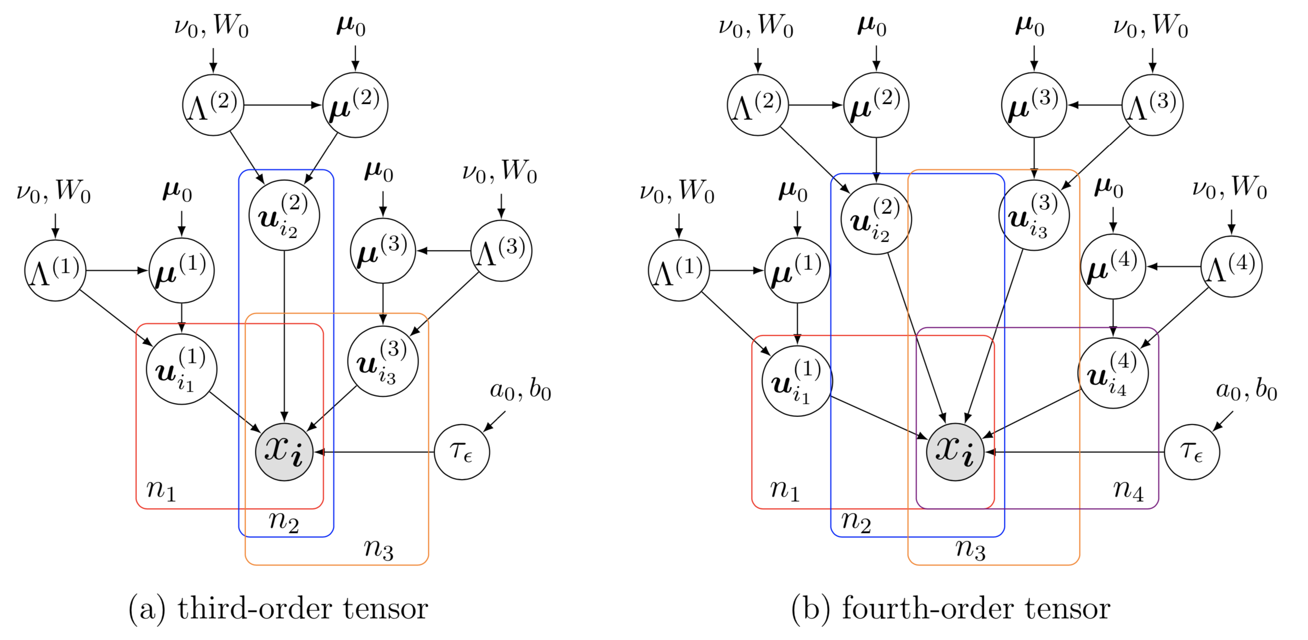
This example is from the following paper:
- Qibin Zhao, Liqing Zhang, Andrzej Cichocki (2015). Bayesian CP factorization of incomplete tensors with automatic rank determination. IEEE Transactions on Pattern Analysis and Machine Intelligence, 37(9): 1751-1763.
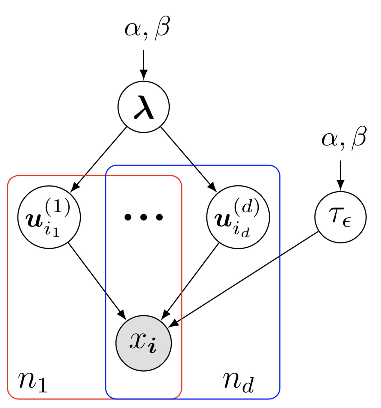 which shows the Bayesian network of Bayesian CP factorization (BCPF) model. To draw this Bayesian network example, there are some preliminaries to follow:
preamble codes:
documentclass as standalone, e.g., \documentclass[border = 0.1cm]{standalone} with 0.1cm border,tikz, i.e., \usepackage{tikz}, and use tikz library like \usetikzlibrary{bayesnet} which is an important tool for drawing Bayesian networks and directed factor graphs,tikz style by using the \tikzstyle{} command,\usepackage{amsfonts, amsmath, amssymb}.body codes:
\begin{tikzpicture} \end{tikzpicture} to start drawing,\node to define nodes and text boxes in the Bayesian network,\path to define arrows in the Bayesian network,\plate to define plates in the Bayesian network.Please click on the image and check out the source code.
This example is from the following paper:
Xinyu Chen, Zhaocheng He, Lijun Sun (2019). A Bayesian tensor decomposition approach for spatiotemporal traffic data imputation. Transportation Research Part C: Emerging Technologies, 98: 73-84.
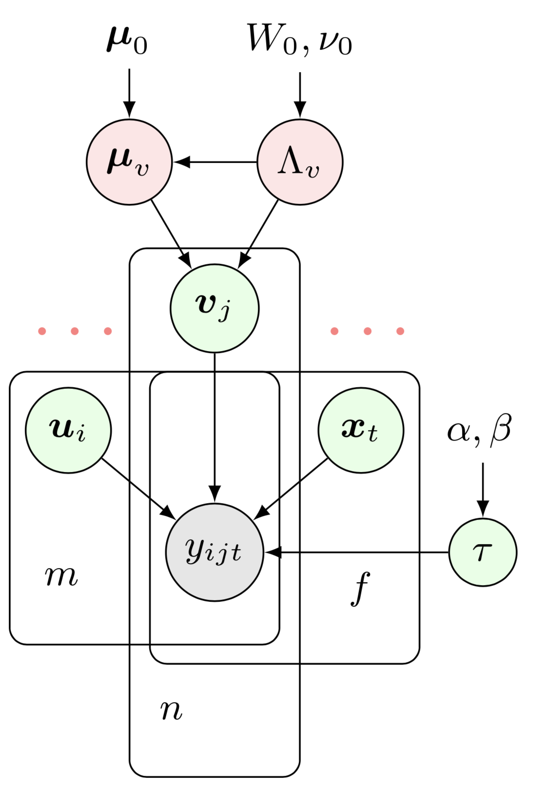 which shows the Bayesian network of Bayesian Gaussian CP factorization (BGCP) model. To draw this Bayesian network example, there are some preliminaries to follow:
preamble codes:
documentclass as standalone, e.g., \documentclass[border = 0.1cm]{standalone} with 0.1cm border,tikz, i.e., \usepackage{tikz}, and use tikz library like \usetikzlibrary{bayesnet} which is an important tool for drawing Bayesian networks and directed factor graph,tikz style by using the \tikzstyle{} command,\usepackage{amsmath, amsfonts, amssymb}.body codes:
\begin{tikzpicture} \end{tikzpicture} to start drawing,\node to define nodes and text boxes in the Bayesian network,\path to define arrows in the Bayesian network,\plate to define plates in the Bayesian network.Please click on the image and check out the source code. If you are interested in the original Bayesian network of BGCP in the paper, please check out BGCP.tex.
This example is from the following paper:
Xinyu Chen, Zhaocheng He, Yixian Chen, Yuhuan Lu, Jiawei Wang (2019). Missing traffic data imputation and pattern discovery with a Bayesian augmented tensor factorization model. Transportation Research Part C: Emerging Technologies, 104: 66-77.
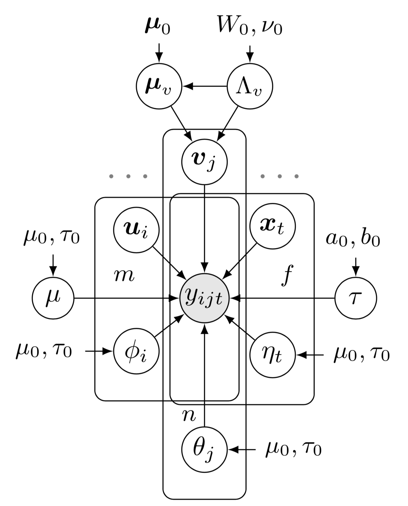 which shows the Bayesian network of Bayesian augmented tensor factorization (BATF) model. To draw this Bayesian network example, there are some preliminaries to follow:
preamble codes:
documentclass as standalone, e.g., \documentclass[border = 0.1cm]{standalone} with 0.1cm border,tikz, i.e., \usepackage{tikz}, and use tikz library like \usetikzlibrary{bayesnet} which is an important tool for drawing Bayesian networks and directed factor graph,tikz style by using the \tikzstyle{} command,\usepackage{amsmath, amsfonts, amssymb}.body codes:
\begin{tikzpicture} \end{tikzpicture} to start drawing,\node to define nodes and text boxes in the Bayesian network,\path to define arrows in the Bayesian network,\plate to define plates in the Bayesian network.Please click on the image and check out the source code.
This example is from the following paper:
Xinyu Chen, Lijun Sun (2021). Bayesian temporal factorization for multidimensional time series prediction. IEEE Transactions on Pattern Analysis and Machine Intelligence, 44 (9): 4659-4673.
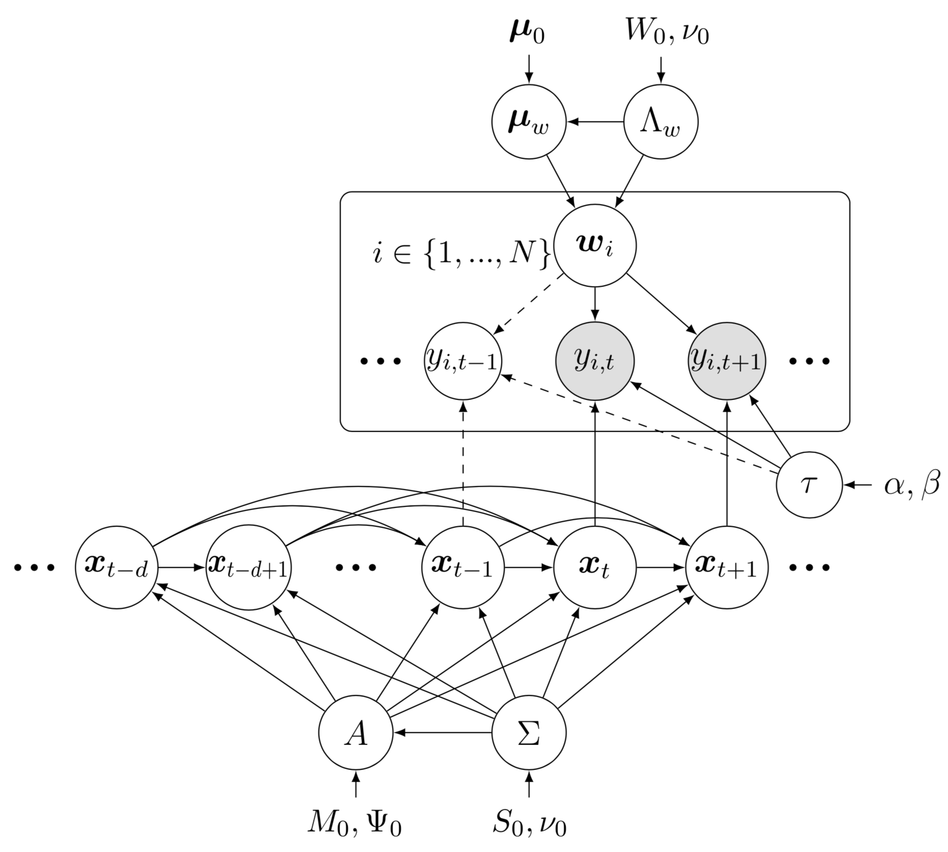 which shows the Bayesian network of Bayesian temporal matrix factorization (BTMF) model. To draw this Bayesian network example, there are some preliminaries to follow:
preamble codes:
documentclass as standalone, e.g., \documentclass[border = 0.1cm]{standalone} with 0.1cm border,tikz, i.e., \usepackage{tikz}, and use tikz library like \usetikzlibrary{bayesnet} which is an important tool for drawing Bayesian networks and directed factor graph,tikz style by using the \tikzstyle{} command,\usepackage{amsmath, amsfonts, amssymb}.body codes:
\begin{tikzpicture} \end{tikzpicture} to start drawing,\node to define nodes and text boxes in the Bayesian network,\path to define arrows in the Bayesian network,\plate to define plates in the Bayesian network.Please click on the image and check out the source code. Instead of multivariate vector autoregressive process on temporal factors, we can also use univariate autoregressive process to rebuild BTMF. The Beyasian network is available at btmf_net.png, you can also check out the source code btmf_net.tex.


These two examples show the partially observed time series matrix and tensor, respectively. To draw both two examples, we can follow these steps:
preamble codes:
documentclass as standalone,tikz.body codes:
\begin{tikzpicture} \end{tikzpicture} to start drawing,\node to define nodes and text boxes in the graphical model,\path to define arrows in the graphical model.


These two examples show the time series prediction in the presence of missing values. To draw both two examples, we can follow these steps:
preamble codes:
documentclass as standalone,tikz.body codes:
\begin{tikzpicture} \end{tikzpicture} to start drawing,\node to define nodes and text boxes in the graphical model,\path to define arrows in the graphical model.


These two examples show the undirected and circulant graphs on the relational data samples with certain degrees. To draw both two examples, we can follow these steps:
preamble codes:
documentclass as standalone,tikz.body codes:
\begin{tikzpicture} \end{tikzpicture} to start drawing,\node to define nodes,\path to define arrows.
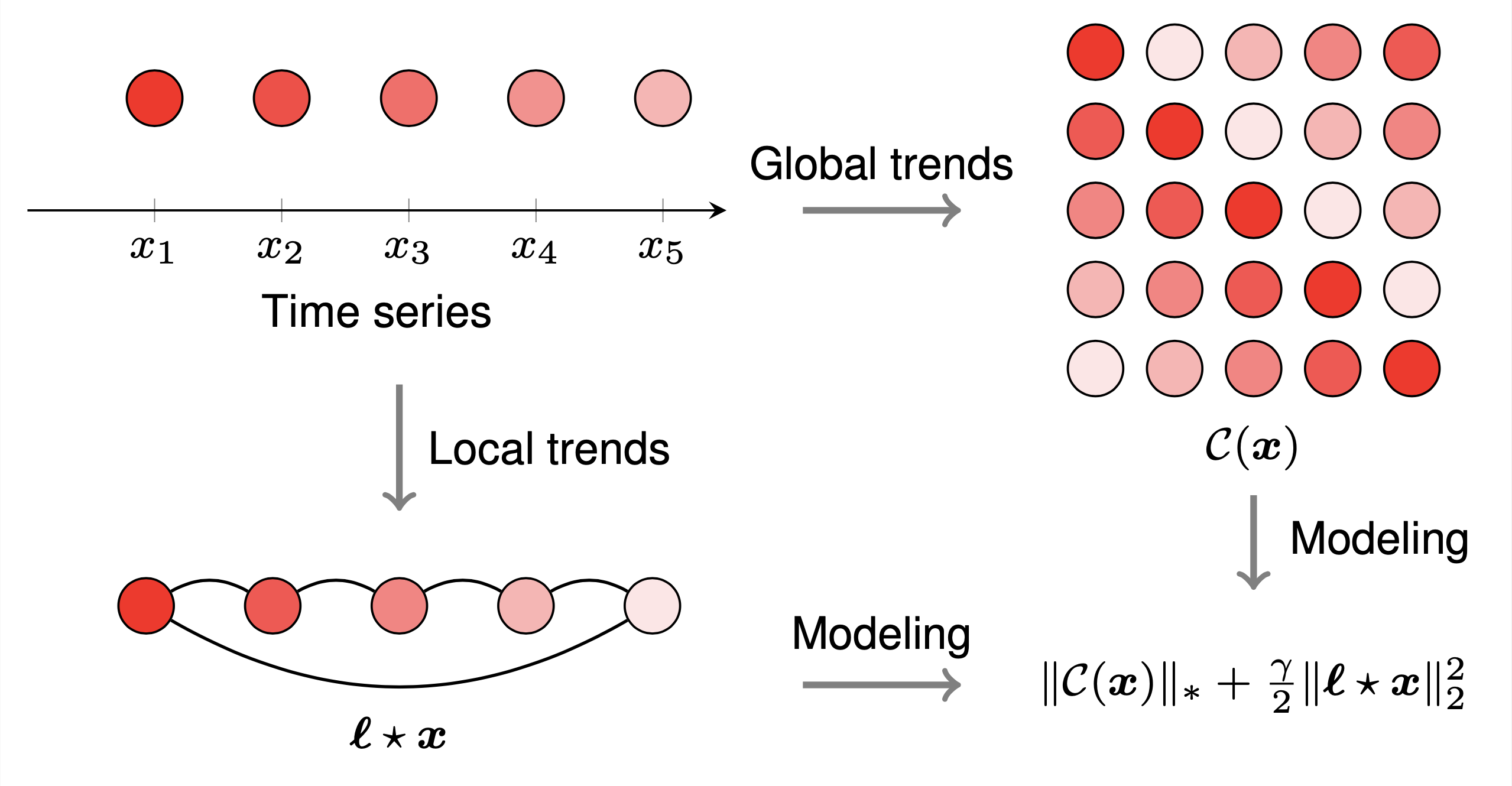
This example is from the following paper:
Xinyu Chen, Zhanhong Cheng, HanQin Cai, Nicolas Saunier, Lijun Sun (2024). Laplacian convolutional representation for traffic time series imputation. IEEE Transactions on Knowledge and Data Engineering. 36 (11): 6490-6502.
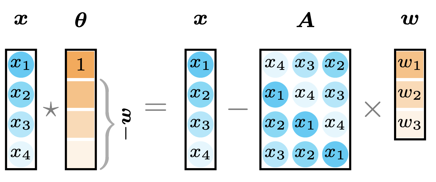
which gives a graphical illustration of the Laplacian convolutional model for time series imputation. To draw the example, we can follow these steps:
preamble codes:
documentclass as standalone,tikz.body codes:
\begin{tikzpicture} \end{tikzpicture} to start drawing,\begin{axis} \end{axis} and \addplot to draw coordinates,\node and \path to draw nodes and arrows.pgfplots Function Plotting
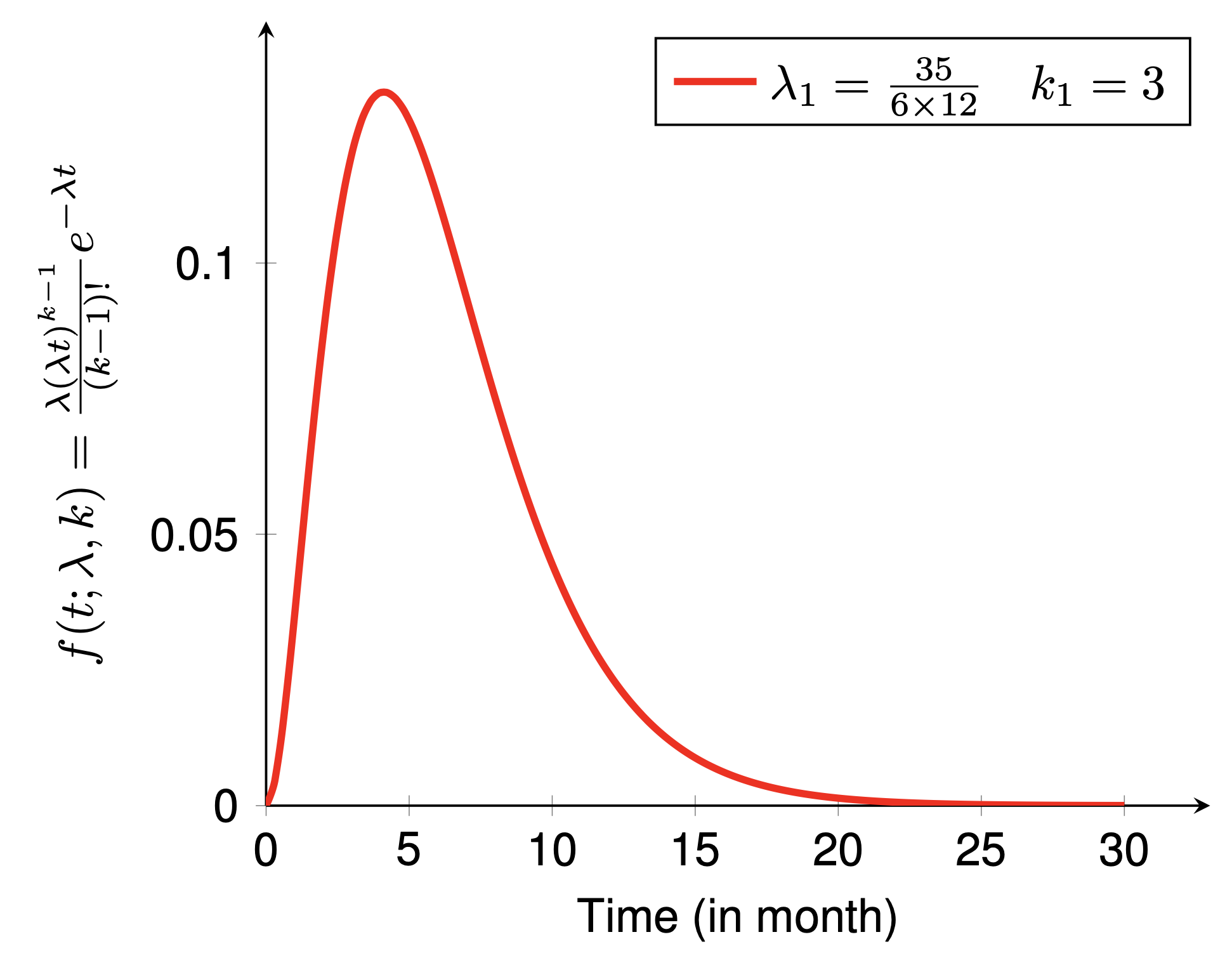
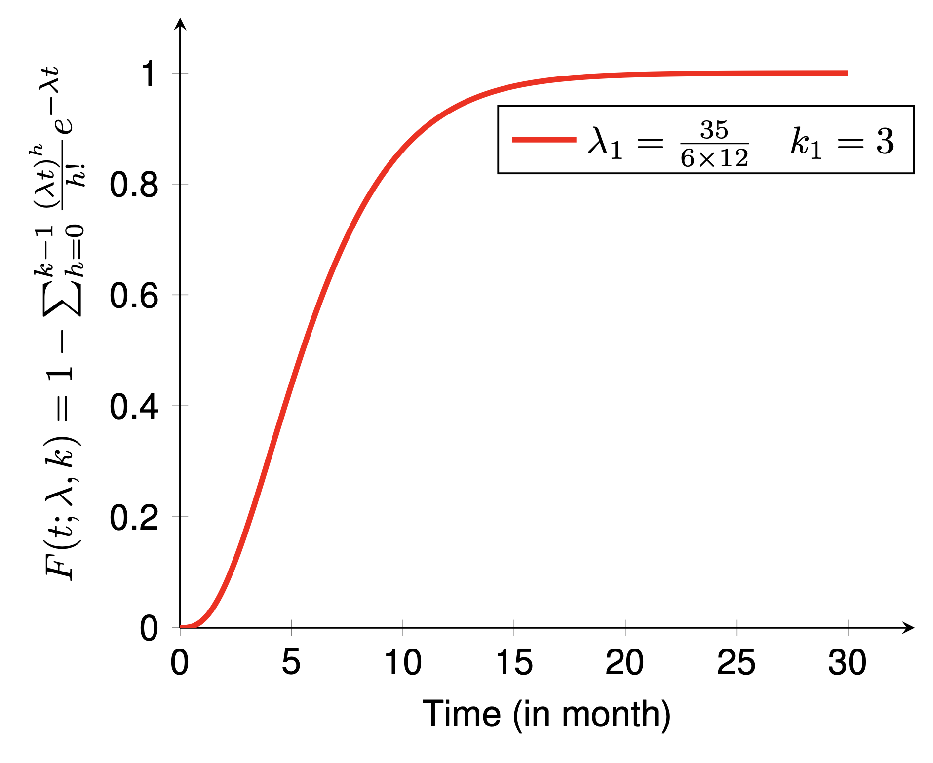
These two examples show the probability density function (PDF) and cumulative density function (CDF) of Erlang distribution, respectively. To draw the example, there are few steps to follow:
preamble codes:
documentclass as standalone,pgfplots,\pgfplotsset{} as you prefer.body codes:
\begin{tikzpicture} \end{tikzpicture} to start drawing,\begin{axis} \end{axis} to draw the function,\addplot to define the function for drawing.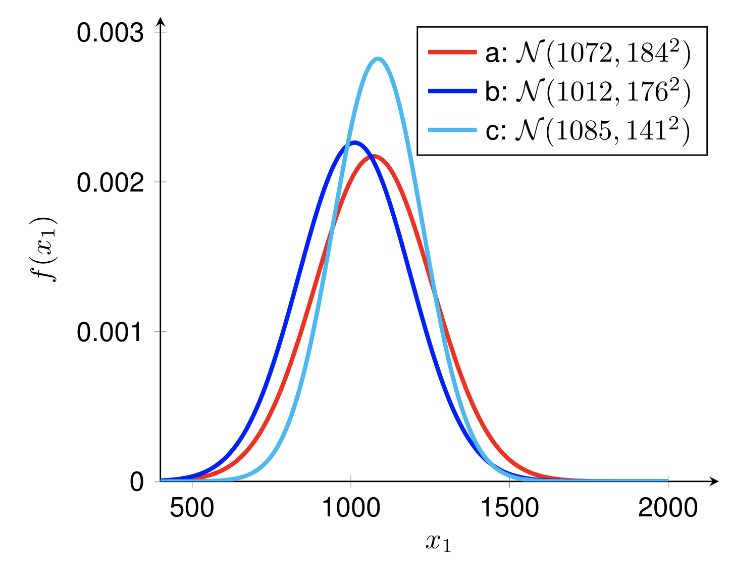
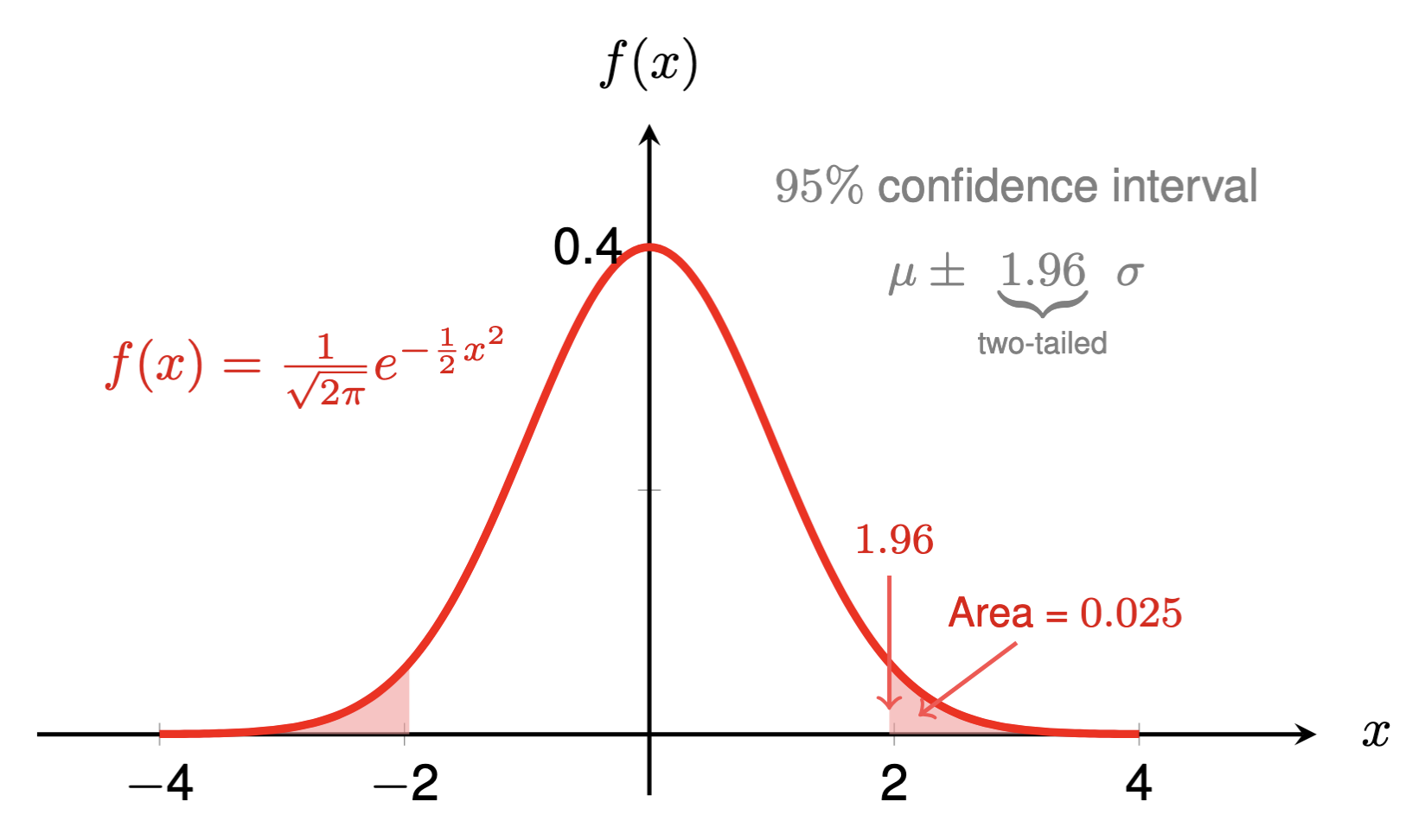
This example shows the PDF of normal distribution with different means and variances. To draw this example, there are few step to follow:
preamble codes:
documentclass as standalone,pgfplots,\pgfplotsset{} as you prefer.body codes:
\pgfmathdeclarefunction to define the PDF function of normal (Gaussian) distribution,\begin{tikzpicture} \end{tikzpicture} to start drawing,\begin{axis} \end{axis} to draw the function,\addplot to define the function for drawing.
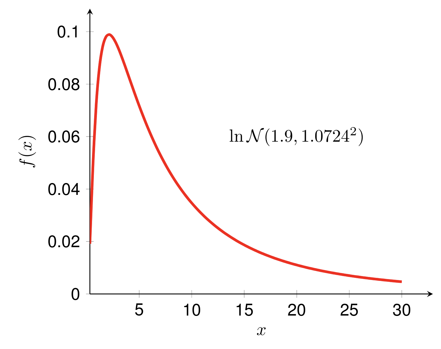
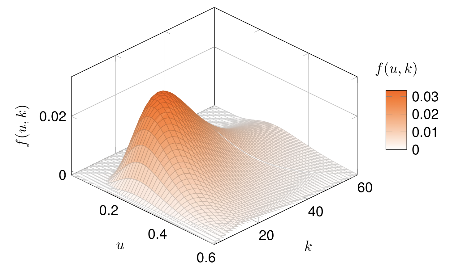
These two examples show the PDF and joint PDF of Lognormal distributions, respectively. There are some recommended material to follow the examples:


These two examples show the iterative process of conjugate gradient for solving a system of linear equations.


These two examples show the random and non-random missing patterns. To draw both two examples, we can follow these steps:
preamble codes:
documentclass as standalone,tikz and pgfplots packages,\begin{filecontents} \end{filecontents} to contain the data.body codes:
\begin{tikzpicture} \end{tikzpicture} to start drawing,\begin{axis} \end{axis} to draw the function,\addplot to draw the data.
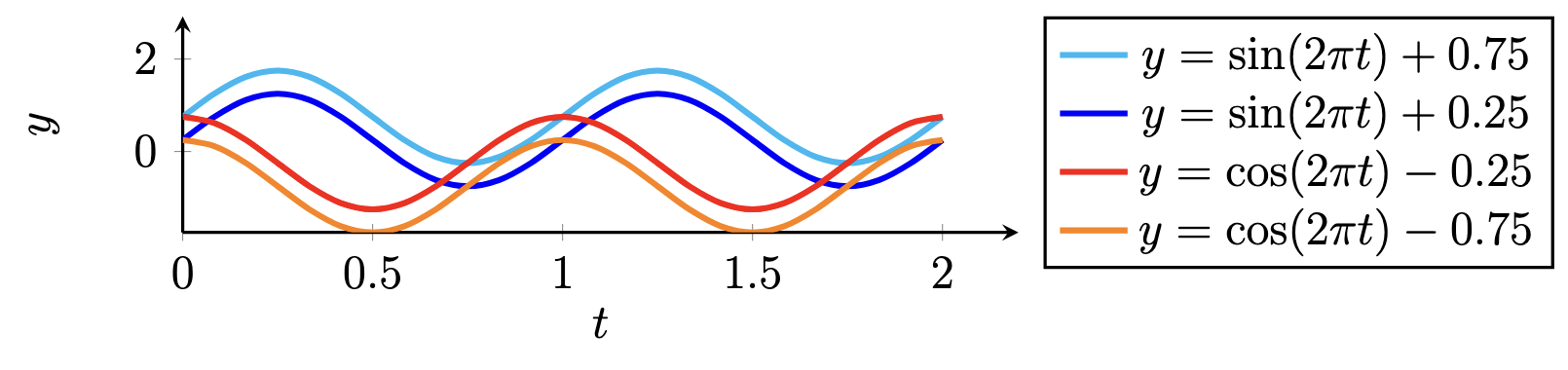
This example shows four sequences consisting of Sine and Cosine functions. When regarding these sequences as time series, then we can see two kinds of temporal dynamics, that is, one is from Sine function, while another is from Cosine function. To draw this example, we can follow these steps:
preamble codes:
documentclass as standalone,pgfplots,\pgfplotsset{} as you prefer.body codes:
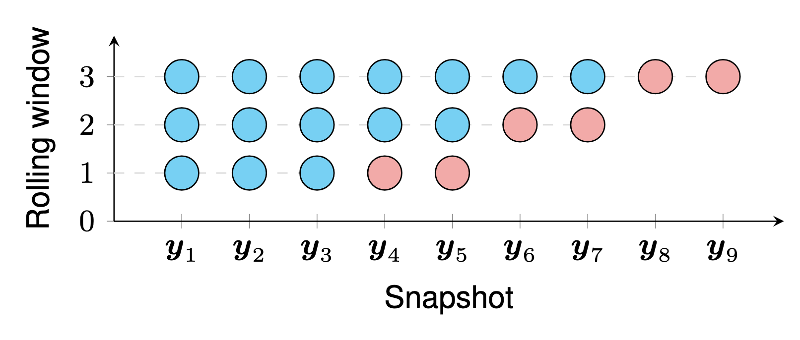
\pgfmathdeclarefunction to define the PDF function of normal (Gaussian) distribution,\begin{tikzpicture} \end{tikzpicture} to start drawing,\begin{axis} \end{axis} to draw the function,\addplot to define the function for drawing.This example illustrates the mechanism of time series forecasting on streaming data in our tracebase project. To draw this example, we can follow these steps:
preamble codes:
documentclass as standalone,tikz and pgfplots packages,\pgfplotsset{} as you prefer.body codes:
\begin{tikzpicture} \end{tikzpicture} to start drawing,\begin{axis} \end{axis} to define the graphic,addplot to define the marks at some coordinates and specify the color of these marks.tikz for Matrix Structure
This example gives a graphical illustration of the multivariate time series forecasting problem with missing values. To draw this example, we can follow these steps:
preamble codes:
documentclass as standalone,tikz.body codes:
\Depth, \Width, and \Height parameters by using \newcommand,\begin{tikzpicture} \end{tikzpicture} to start drawing,\draw, \filldraw, and \node commands to define rectangles and nodes.

This example gives a graphical illustration of the temporal matrix factorization. To draw this example, we can follow these steps:
preamble codes:
documentclass as standalone,tikz.body codes:
\begin{tikzpicture} \end{tikzpicture} to start drawing,\draw and \filldraw to set nodes and rectangles.
This example gives a graphical illustration of the rolling time series forecasting with temporal matrix factorization. To draw this example, we can follow these steps:
preamble codes:
documentclass as standalone,tikz.body codes:
\begin{tikzpicture} \end{tikzpicture} to start drawing,\draw and \filldraw to set nodes and rectangles.tikz-3dplot for Tensor StructureThis example gives a graphical illustration of a third-order tensor. To draw this example, we can follow these steps:
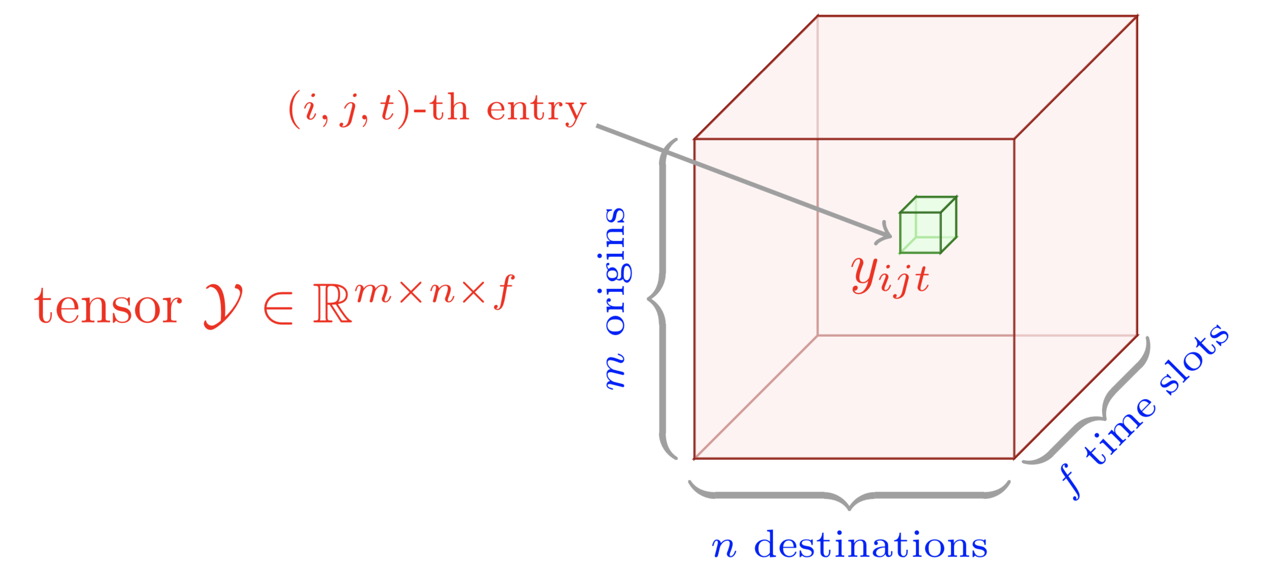
preamble codes:
documentclass as standalone,tikz and tikz-3dplot packages.body codes:
\Depth, \Width, and \Height parameters by using \newcommand,\begin{tikzpicture} \end{tikzpicture} to start drawing,\draw command to define nodes.This example gives a graphical illustration of classical CP tensor factorization on a third-order tensor. To draw this example, we can follow these steps:
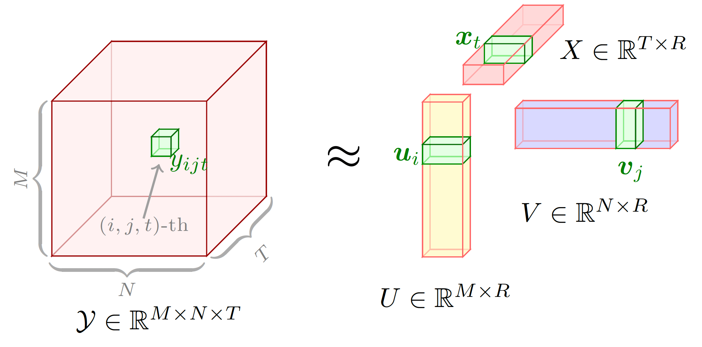
preamble codes:
documentclass as standalone,tikz and tikz-3dplot packages.body codes:
\Depth, \Width, and \Height parameters by using \newcommand,\begin{tikzpicture} \end{tikzpicture} to start drawing,\draw command to define nodes.
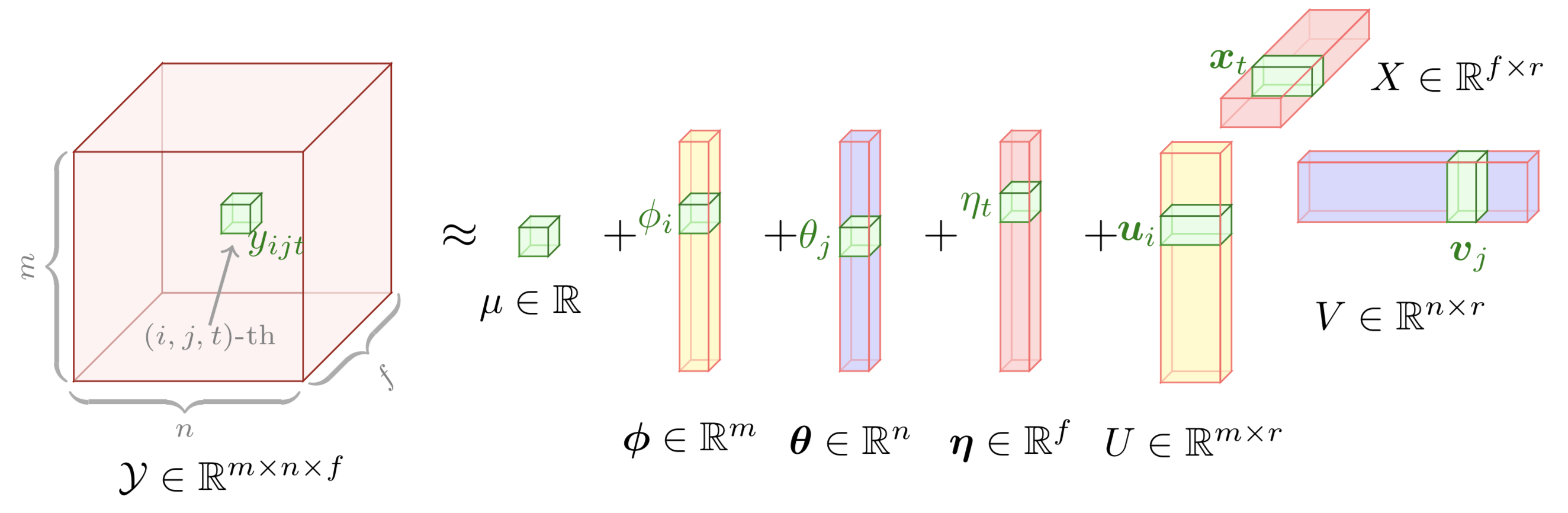
This example gives a graphical illustration of augmented tensor factorization model. To draw this example, we can follow these steps:
preamble codes:
documentclass as standalone,tikz and tikz-3dplot packages.body codes:
\Depth, \Width, and \Height parameters by using \newcommand,\begin{tikzpicture} \end{tikzpicture} to start drawing,\draw command to define nodes.

This example gives a graphical illustration of tensor completion task and its framework including data organization and tensor completion, in which traffic measurements are partially observed. To draw this example, we can follow these steps:
preamble codes:
documentclass as standalone,tikz and tikz-3dplot packages.body codes:
\Depth, \Width, and \Height parameters by using \newcommand,\begin{tikzpicture} \end{tikzpicture} to start drawing,\draw command to define nodes.

This example gives a graphical illustration of low-rank autoregressive tensor completion model. To draw this example, we can follow these steps:
preamble codes:
documentclass as standalone,tikz and tikz-3dplot packages.body codes:
\Depth, \Width, and \Height parameters by using \newcommand,\begin{tikzpicture} \end{tikzpicture} to start drawing,\node, \path, \plate commands to define nodes, arrows, and plates,\draw command to define nodes.This example gives a graphical illustration of singular value thresholding process of the tensor data with unitary transform. To draw this example, we can follow these steps:

preamble codes:
documentclass as standalone,tikz and tikz-3dplot packages.body codes:
\Depth, \Width, and \Height parameters by using \newcommand,\begin{tikzpicture} \end{tikzpicture} to start drawing,\node command to define nodes,\draw command to define nodes,\filldraw command to define colors of rectangles.

This example gives a graphical illustration of low-rank tensor completion model. To draw this example, we can follow these steps:
preamble codes:
documentclass as standalone,tikz and tikz-3dplot packages,algorithm2e package,\usetikzlibrary{positioning, matrix, fit, calc}.body codes:
\begin{algorithm} \end{algorithm} environment to define algorithm,\matrix command to position the components,\begin{scope} \end{scope} to contain the layers.

This example gives a graphical illustration of low-rank tensor regression model. To draw this example, we can follow these steps:
preamble codes:
documentclass as standalone,tikz and tikz-3dplot packages.body codes:
\Depth, \Width, and \Height parameters by using \newcommand,\begin{tikzpicture} \end{tikzpicture} to start drawing,\draw command to define nodes.
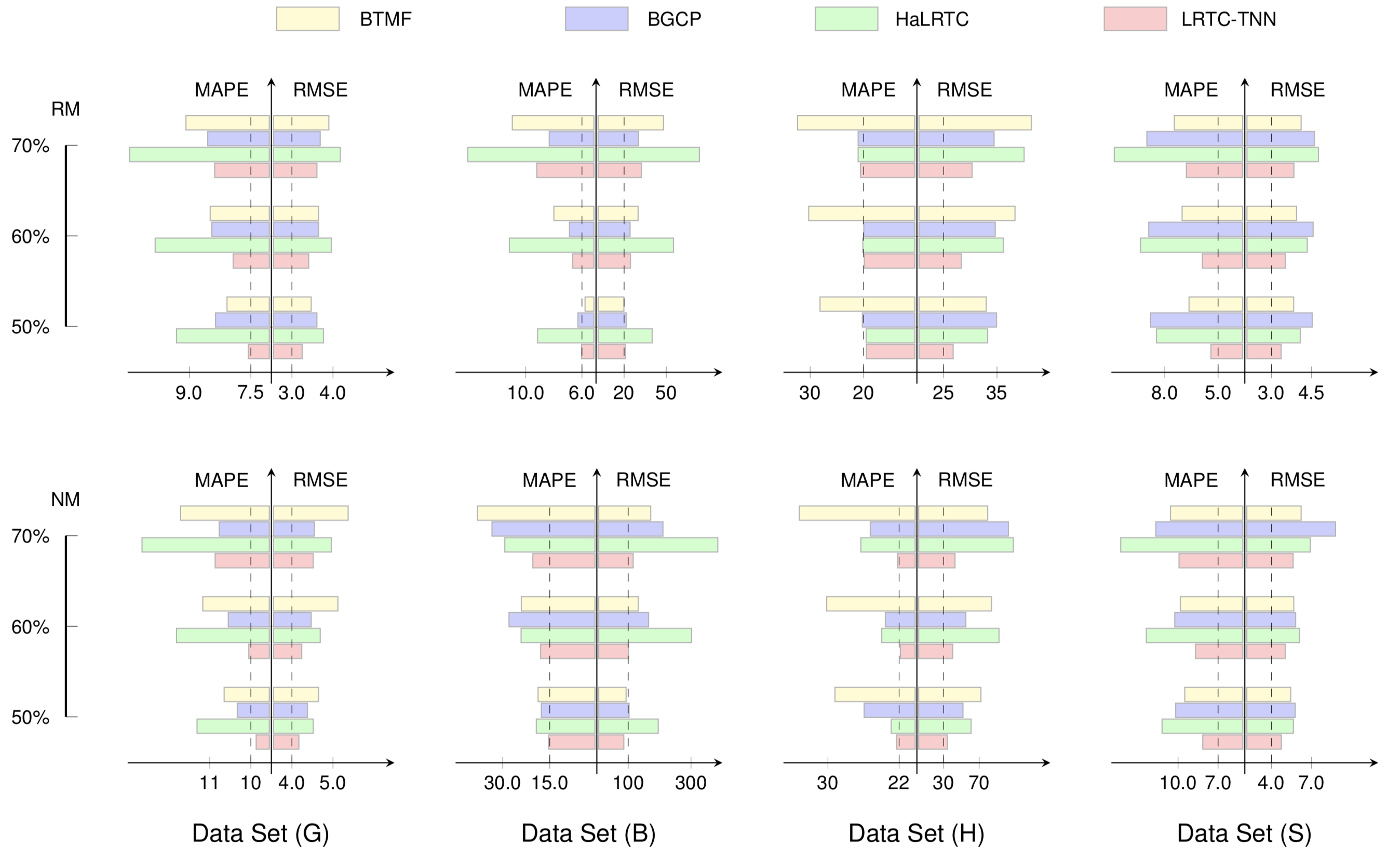
This example shows the imputation accuracy of some matrix and tensor models. To draw this example, we can follow these steps:
preamble codes:
documentclass as standalone,tikz.body codes:
\begin{tikzpicture} \end{tikzpicture} to start drawing,\draw command to define nodes,\pgfuseimage command to import images.
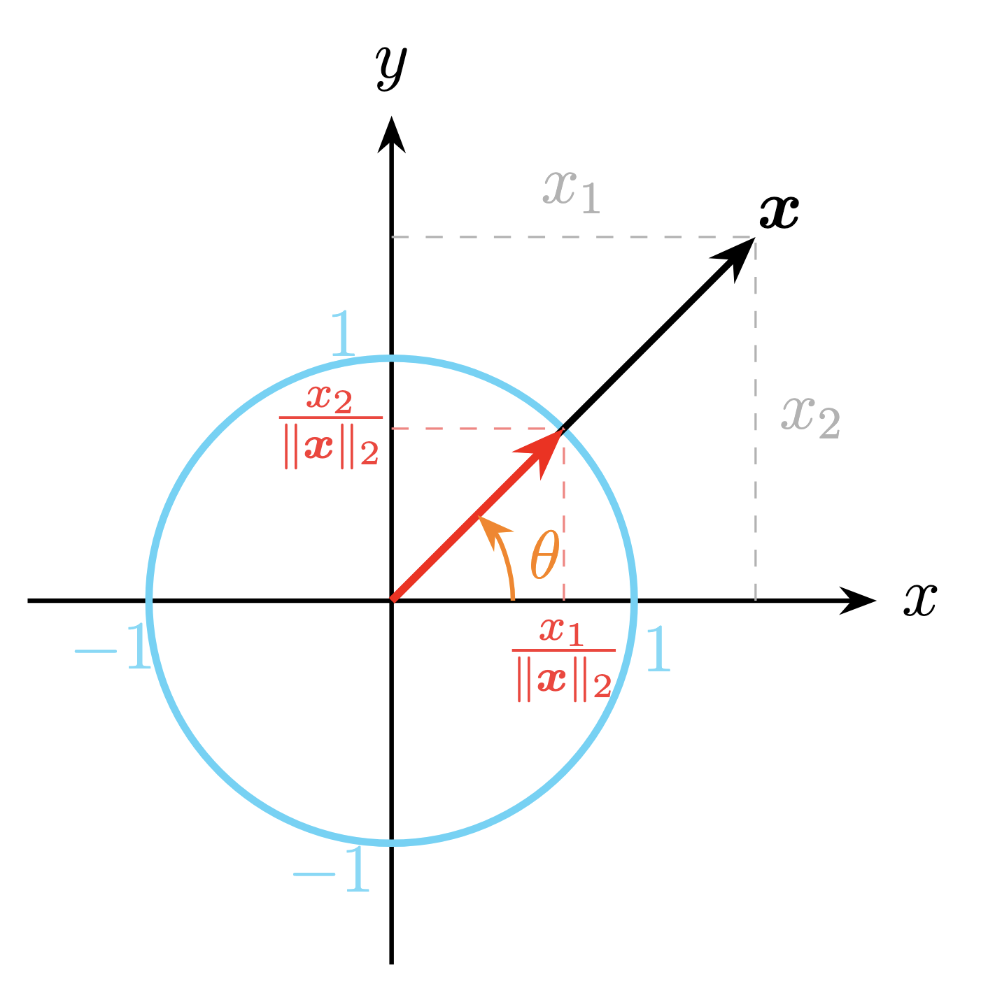
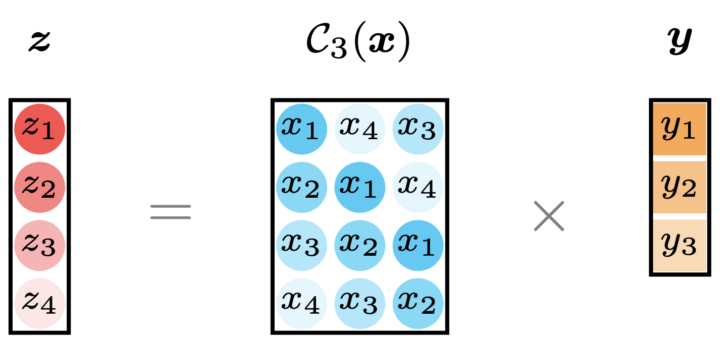
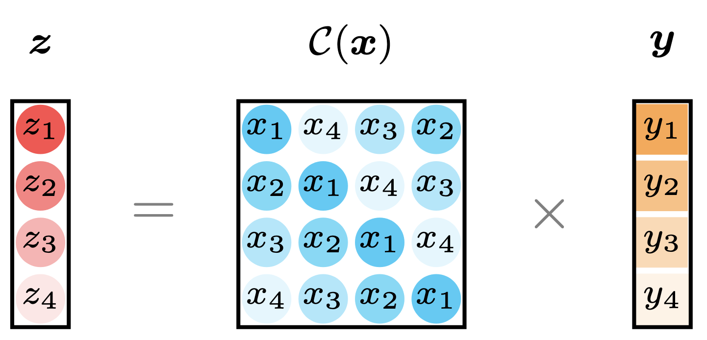
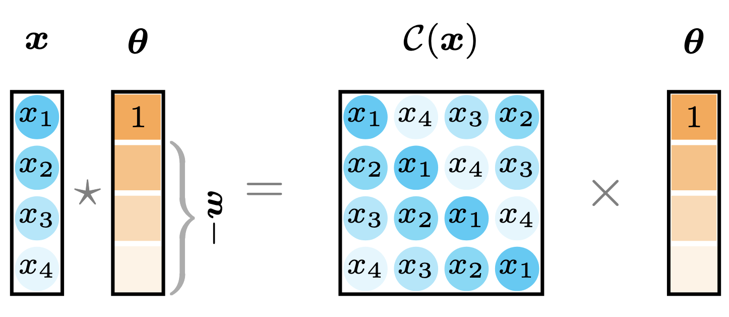
Most of these examples are from our papers:
Xinyu Chen, HanQin Cai, Fuqiang Liu, Jinhua Zhao (2025). Correlating time series with interpretable convolutional kernels. IEEE Transactions on Knowledge and Data Engineering. 37 (6): 3272-3283. [PDF] [DOI] [Blog post] [Data & Python code]
Xinyu Chen, Zhanhong Cheng, HanQin Cai, Nicolas Saunier, Lijun Sun (2024). Laplacian convolutional representation for traffic time series imputation. IEEE Transactions on Knowledge and Data Engineering. 36 (11): 6490-6502. [PDF] [DOI] [Slides] [Blog post] [Data & Python code]
Xinyu Chen, Lijun Sun (2022). Bayesian temporal factorization for multidimensional time series prediction. IEEE Transactions on Pattern Analysis and Machine Intelligence, 44 (9): 4659-4673. [Preprint] [DOI] [Slides] [Data & Python code]
Xinyu Chen, Mengying Lei, Nicolas Saunier, Lijun Sun (2022). Low-rank autoregressive tensor completion for spatiotemporal traffic data imputation. IEEE Transactions on Intelligent Transportation Systems, 23 (8): 12301-12310. [Preprint] [DOI] [Data & Python code] (Also accepted in part to MiLeTS Workshop of KDD 2021, see workshop paper)
Xinyu Chen, Yixian Chen, Nicolas Saunier, Lijun Sun (2021). Scalable low-rank tensor learning for spatiotemporal traffic data imputation. Transportation Research Part C: Emerging Technologies, 129: 103226. [Preprint] [DOI] [Data] [Python code]
Xinyu Chen, Lijun Sun (2020). Low-rank autoregressive tensor completion for multivariate time series forecasting. arXiv preprint arXiv: 2006.10436. [Preprint] [Data & Python code]
Xinyu Chen, Jinming Yang, Lijun Sun (2020). A nonconvex low-rank tensor completion model for spatiotemporal traffic data imputation. Transportation Research Part C: Emerging Technologies, 117: 102673. [Preprint] [DOI] [Data & Python code]
Xinyu Chen, Zhaocheng He, Yixian Chen, Yuhuan Lu, Jiawei Wang (2019). Missing traffic data imputation and pattern discovery with a Bayesian augmented tensor factorization model. Transportation Research Part C: Emerging Technologies, 104: 66-77. [DOI] [Slides] [Data] [Matlab code] [Python code]
Xinyu Chen, Zhaocheng He, Lijun Sun (2019). A Bayesian tensor decomposition approach for spatiotemporal traffic data imputation. Transportation Research Part C: Emerging Technologies, 98: 73-84. [Preprint] [DOI] [Data] [Matlab code] [Python code]
122 followers · starred Sep 2019
164 followers · starred May 2023
24,658 followers · starred Jan 2026
36 followers · starred May 2025
Drawing Bayesian networks, graphical models, tensors, technical frameworks, and illustrations in LaTeX.
See the code
awesome-latex-drawing is a collection of 30+ academic drawing examples for using LaTeX, including Bayesian networks, function plotting, graphical models, matrix/tensor computations, and machine learning frameworks.
LaTeX is a high-quality typesetting system for creating academic graphics. Its popularity stems from its ability to handle complex illustrations with special symbols and mathematical equations, making it ideal for drawing detailed graphics in several scientific areas such as mathematics, physics, and computer science.
This project provides several LaTeX graphics, with examples that are easy to follow on Overleaf. If you are interested, feel free to explore and reproduce our examples on Overleaf at overleaf.com.
Looking for some good LaTeX drawing examples? Here are 30+ graphics for showing how to draw in LaTaX.
LaTeX provides some powerful domain-specific packages and tools like tikz to enable flexible graphical models. Bayesian networks represent a family of graphical models consisting of variables (usually denoted by nodes) and dependency relationships (usually denoted by arrows). Fortunately, tikz has a specific library for drawing Bayesian networks and directed factor graphs.
Another toolbox in Python: https://docs.daft-pgm.org/en/latest/
This example is from the following paper:
- Qibin Zhao, Liqing Zhang, Andrzej Cichocki (2015). Bayesian CP factorization of incomplete tensors with automatic rank determination. IEEE Transactions on Pattern Analysis and Machine Intelligence, 37(9): 1751-1763.
which shows the Bayesian network of Bayesian CP factorization (BCPF) model. To draw this Bayesian network example, there are some preliminaries to follow:
preamble codes:
documentclass as standalone, e.g., \documentclass[border = 0.1cm]{standalone} with 0.1cm border,tikz, i.e., \usepackage{tikz}, and use tikz library like \usetikzlibrary{bayesnet} which is an important tool for drawing Bayesian networks and directed factor graphs,tikz style by using the \tikzstyle{} command,\usepackage{amsfonts, amsmath, amssymb}.body codes:
\begin{tikzpicture} \end{tikzpicture} to start drawing,\node to define nodes and text boxes in the Bayesian network,\path to define arrows in the Bayesian network,\plate to define plates in the Bayesian network.Please click on the image and check out the source code.
This example is from the following paper:
Xinyu Chen, Zhaocheng He, Lijun Sun (2019). A Bayesian tensor decomposition approach for spatiotemporal traffic data imputation. Transportation Research Part C: Emerging Technologies, 98: 73-84.
which shows the Bayesian network of Bayesian Gaussian CP factorization (BGCP) model. To draw this Bayesian network example, there are some preliminaries to follow:
preamble codes:
documentclass as standalone, e.g., \documentclass[border = 0.1cm]{standalone} with 0.1cm border,tikz, i.e., \usepackage{tikz}, and use tikz library like \usetikzlibrary{bayesnet} which is an important tool for drawing Bayesian networks and directed factor graph,tikz style by using the \tikzstyle{} command,\usepackage{amsmath, amsfonts, amssymb}.body codes:
\begin{tikzpicture} \end{tikzpicture} to start drawing,\node to define nodes and text boxes in the Bayesian network,\path to define arrows in the Bayesian network,\plate to define plates in the Bayesian network.Please click on the image and check out the source code. If you are interested in the original Bayesian network of BGCP in the paper, please check out BGCP.tex.
This example is from the following paper:
Xinyu Chen, Zhaocheng He, Yixian Chen, Yuhuan Lu, Jiawei Wang (2019). Missing traffic data imputation and pattern discovery with a Bayesian augmented tensor factorization model. Transportation Research Part C: Emerging Technologies, 104: 66-77.
which shows the Bayesian network of Bayesian augmented tensor factorization (BATF) model. To draw this Bayesian network example, there are some preliminaries to follow:
preamble codes:
documentclass as standalone, e.g., \documentclass[border = 0.1cm]{standalone} with 0.1cm border,tikz, i.e., \usepackage{tikz}, and use tikz library like \usetikzlibrary{bayesnet} which is an important tool for drawing Bayesian networks and directed factor graph,tikz style by using the \tikzstyle{} command,\usepackage{amsmath, amsfonts, amssymb}.body codes:
\begin{tikzpicture} \end{tikzpicture} to start drawing,\node to define nodes and text boxes in the Bayesian network,\path to define arrows in the Bayesian network,\plate to define plates in the Bayesian network.Please click on the image and check out the source code.
This example is from the following paper:
Xinyu Chen, Lijun Sun (2021). Bayesian temporal factorization for multidimensional time series prediction. IEEE Transactions on Pattern Analysis and Machine Intelligence, 44 (9): 4659-4673.
which shows the Bayesian network of Bayesian temporal matrix factorization (BTMF) model. To draw this Bayesian network example, there are some preliminaries to follow:
preamble codes:
documentclass as standalone, e.g., \documentclass[border = 0.1cm]{standalone} with 0.1cm border,tikz, i.e., \usepackage{tikz}, and use tikz library like \usetikzlibrary{bayesnet} which is an important tool for drawing Bayesian networks and directed factor graph,tikz style by using the \tikzstyle{} command,\usepackage{amsmath, amsfonts, amssymb}.body codes:
\begin{tikzpicture} \end{tikzpicture} to start drawing,\node to define nodes and text boxes in the Bayesian network,\path to define arrows in the Bayesian network,\plate to define plates in the Bayesian network.Please click on the image and check out the source code. Instead of multivariate vector autoregressive process on temporal factors, we can also use univariate autoregressive process to rebuild BTMF. The Beyasian network is available at btmf_net.png, you can also check out the source code btmf_net.tex.
These two examples show the partially observed time series matrix and tensor, respectively. To draw both two examples, we can follow these steps:
preamble codes:
documentclass as standalone,tikz.body codes:
\begin{tikzpicture} \end{tikzpicture} to start drawing,\node to define nodes and text boxes in the graphical model,\path to define arrows in the graphical model.
These two examples show the time series prediction in the presence of missing values. To draw both two examples, we can follow these steps:
preamble codes:
documentclass as standalone,tikz.body codes:
\begin{tikzpicture} \end{tikzpicture} to start drawing,\node to define nodes and text boxes in the graphical model,\path to define arrows in the graphical model.
These two examples show the undirected and circulant graphs on the relational data samples with certain degrees. To draw both two examples, we can follow these steps:
preamble codes:
documentclass as standalone,tikz.body codes:
\begin{tikzpicture} \end{tikzpicture} to start drawing,\node to define nodes,\path to define arrows.
This example is from the following paper:
Xinyu Chen, Zhanhong Cheng, HanQin Cai, Nicolas Saunier, Lijun Sun (2024). Laplacian convolutional representation for traffic time series imputation. IEEE Transactions on Knowledge and Data Engineering. 36 (11): 6490-6502.
which gives a graphical illustration of the Laplacian convolutional model for time series imputation. To draw the example, we can follow these steps:
preamble codes:
documentclass as standalone,tikz.body codes:
\begin{tikzpicture} \end{tikzpicture} to start drawing,\begin{axis} \end{axis} and \addplot to draw coordinates,\node and \path to draw nodes and arrows.pgfplots Function Plotting
These two examples show the probability density function (PDF) and cumulative density function (CDF) of Erlang distribution, respectively. To draw the example, there are few steps to follow:
preamble codes:
documentclass as standalone,pgfplots,\pgfplotsset{} as you prefer.body codes:
\begin{tikzpicture} \end{tikzpicture} to start drawing,\begin{axis} \end{axis} to draw the function,\addplot to define the function for drawing.
This example shows the PDF of normal distribution with different means and variances. To draw this example, there are few step to follow:
preamble codes:
documentclass as standalone,pgfplots,\pgfplotsset{} as you prefer.body codes:
\pgfmathdeclarefunction to define the PDF function of normal (Gaussian) distribution,\begin{tikzpicture} \end{tikzpicture} to start drawing,\begin{axis} \end{axis} to draw the function,\addplot to define the function for drawing.
These two examples show the PDF and joint PDF of Lognormal distributions, respectively. There are some recommended material to follow the examples:
These two examples show the iterative process of conjugate gradient for solving a system of linear equations.
These two examples show the random and non-random missing patterns. To draw both two examples, we can follow these steps:
preamble codes:
documentclass as standalone,tikz and pgfplots packages,\begin{filecontents} \end{filecontents} to contain the data.body codes:
\begin{tikzpicture} \end{tikzpicture} to start drawing,\begin{axis} \end{axis} to draw the function,\addplot to draw the data.
This example shows four sequences consisting of Sine and Cosine functions. When regarding these sequences as time series, then we can see two kinds of temporal dynamics, that is, one is from Sine function, while another is from Cosine function. To draw this example, we can follow these steps:
preamble codes:
documentclass as standalone,pgfplots,\pgfplotsset{} as you prefer.body codes:
\pgfmathdeclarefunction to define the PDF function of normal (Gaussian) distribution,\begin{tikzpicture} \end{tikzpicture} to start drawing,\begin{axis} \end{axis} to draw the function,\addplot to define the function for drawing.This example illustrates the mechanism of time series forecasting on streaming data in our tracebase project. To draw this example, we can follow these steps:
preamble codes:
documentclass as standalone,tikz and pgfplots packages,\pgfplotsset{} as you prefer.body codes:
\begin{tikzpicture} \end{tikzpicture} to start drawing,\begin{axis} \end{axis} to define the graphic,addplot to define the marks at some coordinates and specify the color of these marks.tikz for Matrix Structure
This example gives a graphical illustration of the multivariate time series forecasting problem with missing values. To draw this example, we can follow these steps:
preamble codes:
documentclass as standalone,tikz.body codes:
\Depth, \Width, and \Height parameters by using \newcommand,\begin{tikzpicture} \end{tikzpicture} to start drawing,\draw, \filldraw, and \node commands to define rectangles and nodes.
This example gives a graphical illustration of the temporal matrix factorization. To draw this example, we can follow these steps:
preamble codes:
documentclass as standalone,tikz.body codes:
\begin{tikzpicture} \end{tikzpicture} to start drawing,\draw and \filldraw to set nodes and rectangles.
This example gives a graphical illustration of the rolling time series forecasting with temporal matrix factorization. To draw this example, we can follow these steps:
preamble codes:
documentclass as standalone,tikz.body codes:
\begin{tikzpicture} \end{tikzpicture} to start drawing,\draw and \filldraw to set nodes and rectangles.tikz-3dplot for Tensor StructureThis example gives a graphical illustration of a third-order tensor. To draw this example, we can follow these steps:
preamble codes:
documentclass as standalone,tikz and tikz-3dplot packages.body codes:
\Depth, \Width, and \Height parameters by using \newcommand,\begin{tikzpicture} \end{tikzpicture} to start drawing,\draw command to define nodes.This example gives a graphical illustration of classical CP tensor factorization on a third-order tensor. To draw this example, we can follow these steps:
preamble codes:
documentclass as standalone,tikz and tikz-3dplot packages.body codes:
\Depth, \Width, and \Height parameters by using \newcommand,\begin{tikzpicture} \end{tikzpicture} to start drawing,\draw command to define nodes.
This example gives a graphical illustration of augmented tensor factorization model. To draw this example, we can follow these steps:
preamble codes:
documentclass as standalone,tikz and tikz-3dplot packages.body codes:
\Depth, \Width, and \Height parameters by using \newcommand,\begin{tikzpicture} \end{tikzpicture} to start drawing,\draw command to define nodes.
This example gives a graphical illustration of tensor completion task and its framework including data organization and tensor completion, in which traffic measurements are partially observed. To draw this example, we can follow these steps:
preamble codes:
documentclass as standalone,tikz and tikz-3dplot packages.body codes:
\Depth, \Width, and \Height parameters by using \newcommand,\begin{tikzpicture} \end{tikzpicture} to start drawing,\draw command to define nodes.
This example gives a graphical illustration of low-rank autoregressive tensor completion model. To draw this example, we can follow these steps:
preamble codes:
documentclass as standalone,tikz and tikz-3dplot packages.body codes:
\Depth, \Width, and \Height parameters by using \newcommand,\begin{tikzpicture} \end{tikzpicture} to start drawing,\node, \path, \plate commands to define nodes, arrows, and plates,\draw command to define nodes.This example gives a graphical illustration of singular value thresholding process of the tensor data with unitary transform. To draw this example, we can follow these steps:
preamble codes:
documentclass as standalone,tikz and tikz-3dplot packages.body codes:
\Depth, \Width, and \Height parameters by using \newcommand,\begin{tikzpicture} \end{tikzpicture} to start drawing,\node command to define nodes,\draw command to define nodes,\filldraw command to define colors of rectangles.
This example gives a graphical illustration of low-rank tensor completion model. To draw this example, we can follow these steps:
preamble codes:
documentclass as standalone,tikz and tikz-3dplot packages,algorithm2e package,\usetikzlibrary{positioning, matrix, fit, calc}.body codes:
\begin{algorithm} \end{algorithm} environment to define algorithm,\matrix command to position the components,\begin{scope} \end{scope} to contain the layers.
This example gives a graphical illustration of low-rank tensor regression model. To draw this example, we can follow these steps:
preamble codes:
documentclass as standalone,tikz and tikz-3dplot packages.body codes:
\Depth, \Width, and \Height parameters by using \newcommand,\begin{tikzpicture} \end{tikzpicture} to start drawing,\draw command to define nodes.
This example shows the imputation accuracy of some matrix and tensor models. To draw this example, we can follow these steps:
preamble codes:
documentclass as standalone,tikz.body codes:
\begin{tikzpicture} \end{tikzpicture} to start drawing,\draw command to define nodes,\pgfuseimage command to import images.
Most of these examples are from our papers:
Xinyu Chen, HanQin Cai, Fuqiang Liu, Jinhua Zhao (2025). Correlating time series with interpretable convolutional kernels. IEEE Transactions on Knowledge and Data Engineering. 37 (6): 3272-3283. [PDF] [DOI] [Blog post] [Data & Python code]
Xinyu Chen, Zhanhong Cheng, HanQin Cai, Nicolas Saunier, Lijun Sun (2024). Laplacian convolutional representation for traffic time series imputation. IEEE Transactions on Knowledge and Data Engineering. 36 (11): 6490-6502. [PDF] [DOI] [Slides] [Blog post] [Data & Python code]
Xinyu Chen, Lijun Sun (2022). Bayesian temporal factorization for multidimensional time series prediction. IEEE Transactions on Pattern Analysis and Machine Intelligence, 44 (9): 4659-4673. [Preprint] [DOI] [Slides] [Data & Python code]
Xinyu Chen, Mengying Lei, Nicolas Saunier, Lijun Sun (2022). Low-rank autoregressive tensor completion for spatiotemporal traffic data imputation. IEEE Transactions on Intelligent Transportation Systems, 23 (8): 12301-12310. [Preprint] [DOI] [Data & Python code] (Also accepted in part to MiLeTS Workshop of KDD 2021, see workshop paper)
Xinyu Chen, Yixian Chen, Nicolas Saunier, Lijun Sun (2021). Scalable low-rank tensor learning for spatiotemporal traffic data imputation. Transportation Research Part C: Emerging Technologies, 129: 103226. [Preprint] [DOI] [Data] [Python code]
Xinyu Chen, Lijun Sun (2020). Low-rank autoregressive tensor completion for multivariate time series forecasting. arXiv preprint arXiv: 2006.10436. [Preprint] [Data & Python code]
Xinyu Chen, Jinming Yang, Lijun Sun (2020). A nonconvex low-rank tensor completion model for spatiotemporal traffic data imputation. Transportation Research Part C: Emerging Technologies, 117: 102673. [Preprint] [DOI] [Data & Python code]
Xinyu Chen, Zhaocheng He, Yixian Chen, Yuhuan Lu, Jiawei Wang (2019). Missing traffic data imputation and pattern discovery with a Bayesian augmented tensor factorization model. Transportation Research Part C: Emerging Technologies, 104: 66-77. [DOI] [Slides] [Data] [Matlab code] [Python code]
Xinyu Chen, Zhaocheng He, Lijun Sun (2019). A Bayesian tensor decomposition approach for spatiotemporal traffic data imputation. Transportation Research Part C: Emerging Technologies, 98: 73-84. [Preprint] [DOI] [Data] [Matlab code] [Python code]
122 followers · starred Sep 2019
164 followers · starred May 2023
24,658 followers · starred Jan 2026
36 followers · starred May 2025