


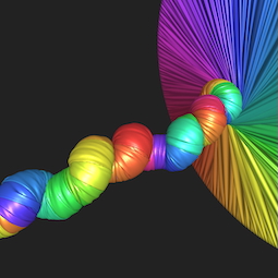
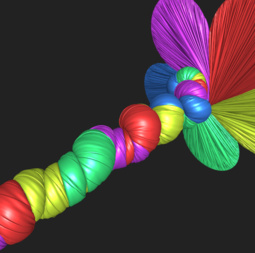
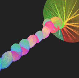
A contact solver for physics-based simulations involving 👚 shells, 🪵 solids, 🪢 rods, 🧱 rigid bodies and ⏳ sand.
Python
4,550
462 commits
updated Oct 8, 2026
A contact solver for physics-based simulations involving 👚 shells, 🪵 solids, 🪢 rods, 🧱 rigid bodies and ⏳ sand. Started as an in-house physics engine at ZOZO, Inc., the largest fashion e-commerce company in Japan, and now evolving with the community. All open-source.


🤖 LLM Transparency: We highly respect that readers expect to hear the author's original voice and tone, which we work to retain throughout. Our use of LLMs is clarified in (Markdown).
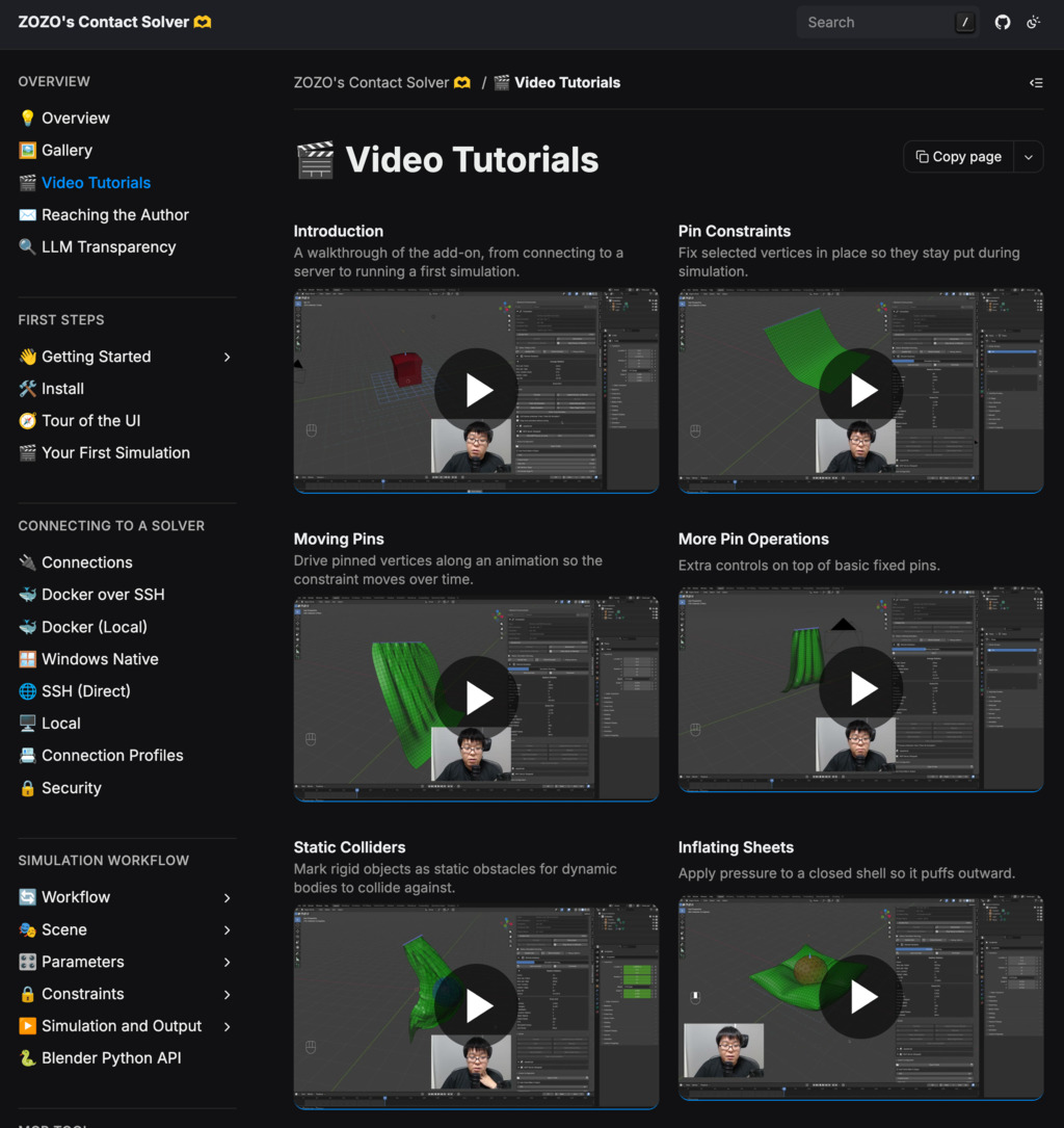
If you simply want to use this through Blender, watch this CGMatter YouTube video. The release page is here. Our video tutorials page is here.
🎨 Simulate remotely from our Blender add-on (screenshots taken on macOS; you can also run locally on a modern NVIDIA GPU on Windows or Linux, or on an Apple silicon Mac)
https://github.com/user-attachments/assets/f266111e-7380-428b-8a3c-25eac4f039e5
🚀 Or run it locally: ./ppf-contact-solver (macOS/Linux), double click start.bat (Windows), or a Docker command (Linux/Windows)

🌐 Click the URL and explore our examples

📚 For the complete change history, see articles/changes.md.
https://github.com/user-attachments/assets/ac104255-604e-4890-9fb1-59732f004f0a
The main branch is undergoing frequent updates and will deviate from the paper.
To retain consistency with the paper, we have created a new branch sigasia-2024.
ghcr.io/st-tech/ppf-contact-solver-compiled-sigasia-2024:latest of this branch.A GPU is recommended, but not required. The right backend is picked for you when a run starts.
| Hardware | Backend | Runs on | Good to know |
|---|---|---|---|
| 🟩 NVIDIA GPU | CUDA 12.8+ | Linux (x86_64, arm64), Windows (x86_64) | RTX 4090 / 5090 for large scenes; 3090 / 4070 / 5070 for small to medium ones |
| 🟥 AMD GPU | ROCm | Linux (x86_64), Windows (x86_64) | gfx9 through gfx12 |
| 🍎 Apple silicon | Metal | macOS | M1 / A14 generation or newer |
| 💻 Any CPU | CPU (x86_64, arm64) | macOS, Windows, Linux | SIMD-optimized using AVX2 and NEON instructions |
You will also need:
Whether you plan to use the Blender add-on or the JupyterLab interface, the solver engine itself must first be deployed. The steps below apply to both.
⚠️ Do not run
warmup.pylocally. If you do, you are very likely to hit failures and find it difficult to cleanup.
🤔 If you are cautious, you can review the build workflow to verify safety yourself. We try to maximize transparency; we never build locally and upload.
For Apple silicon Macs, a self-contained folder carrying the Metal and CPU backends. No Python, Homebrew, or Xcode installation is needed, and nothing is installed outside the folder.
./ppf-contact-solverJupyterLab frontend will auto-start. You should be able to access it at http://localhost:8080.
Keep the terminal window open; Ctrl+C shuts it down.
For Windows 10/11 users, a self-contained executable (several hundred MB) is available. No Python, Docker, or CUDA Toolkit installation is needed. All should simply work out of the box (Video). The x86_64 archive carries the CUDA, ROCm, and CPU backends, so one download serves an NVIDIA machine and an AMD one, while a Windows on ARM machine runs the CPU backend.
start.batJupyterLab frontend will auto-start. You should be able to access it at http://localhost:8080.
A self-contained directory for x86_64 and aarch64 machines running glibc 2.28 or newer. The x86_64 archive carries the CUDA, ROCm, and CPU backends, and the aarch64 one carries CUDA and the CPU backend. No Python, CUDA Toolkit, or ROCm installation is needed.
./ppf-contact-solverJupyterLab frontend will auto-start. You should be able to access it at http://localhost:8080.
Keep the terminal window open; Ctrl+C shuts it down.
Install a NVIDIA driver (Link) on your host system and follow the instructions below specific to the operating system to get a Docker running:
| 🐧 Linux | 🪟 Windows |
|---|---|
Install the Docker engine from here (Link). Also, install the NVIDIA Container Toolkit (Link). Just to make sure that the Container Toolkit is loaded, run sudo service docker restart. | Install the Docker Desktop (Link). You may need to log out or reboot after the installation. After logging back in, launch Docker Desktop to ensure that Docker is running. |
Next, run the following command to start the container. If no edits are needed, just copy and paste:
$MY_WEB_PORT = 8080      # JupyterLab port on your side
$MY_BLENDER_PORT = 9090  # Solver port for the Blender add-on
$IMAGE_NAME = "ghcr.io/st-tech/ppf-contact-solver-compiled:latest"
docker run --rm -it `
  --name ppf-contact-solver `
  --gpus all `
  -p ${MY_WEB_PORT}:${MY_WEB_PORT} `
  -p ${MY_BLENDER_PORT}:${MY_BLENDER_PORT} `
  -e WEB_PORT=${MY_WEB_PORT} `
  $IMAGE_NAME # Image size ~1GB
MY_WEB_PORT=8080      # JupyterLab port on your side
MY_BLENDER_PORT=9090  # Solver port for the Blender add-on
IMAGE_NAME=ghcr.io/st-tech/ppf-contact-solver-compiled:latest
docker run --rm -it \
  --name ppf-contact-solver \
  --gpus all \
  -p ${MY_WEB_PORT}:${MY_WEB_PORT} \
  -p ${MY_BLENDER_PORT}:${MY_BLENDER_PORT} \
  -e WEB_PORT=${MY_WEB_PORT} \
  $IMAGE_NAME # Image size ~1GB
The image download shall be started. Our image is hosted on GitHub Container Registry (~1GB). JupyterLab will then auto-start. Eventually you should be seeing:
==== JupyterLab Launched! 🚀 ====
     http://localhost:8080
    Press Ctrl+C to shutdown
================================
Next, open your browser and navigate to http://localhost:8080. The port 8080 can change if you change the MY_WEB_PORT variable.
Keep your terminal window open.
Now you are ready to go! 🎉
To shut down the container, just press Ctrl+C in the terminal.
The container will be removed and all traces will be cleaned up. 🧹
If you wish to keep the container running in the background, replace
--rmwith-d. To shutdown the container and remove it, rundocker stop ppf-contact-solver && docker rm ppf-contact-solver.
If you wish to build the docker image from scratch, please refer to the cleaner installation guide (Markdown).
We provide two frontends: a Blender add-on and a JupyterLab interface. The Blender add-on lets you build scenes and run simulations entirely within Blender's UI, while JupyterLab lets you script everything in Python from your browser. Both communicate with the same solver engine, so pick whichever you like.
In both cases, you can interact with the simulator on your laptop while the actual simulation runs on a remote headless server over the internet. This means that you don't have to own NVIDIA hardware, but can rent it at vast.ai for less than $0.5 per hour. That said, if you do have a modern NVIDIA GPU on a local Windows or Linux machine, or an Apple silicon Mac, you can also run the solver directly on it. Actually, this (Video) was recorded on a vast.ai instance. The experience is good! 👍
Our Blender add-on aims to offer a familiar UI that best feels like everything works locally, but under the hood, it communicates with a remote server where all simulations run, and then the results are fetched back.
This provides a unique experience where users can leverage powerful remote GPUs while working seamlessly in their local Blender environment. Remarkably, our Blender add-on works even on macOS systems 😊, unlike other CUDA-based physics simulator add-ons that require local NVIDIA GPUs. More importantly, you can work on a laptop without worrying about draining the battery fast. 🔋
Follow this page How to Install to learn how to install the add-on. For a thorough walk through workflow, we refer to our documentation below:

🎬 Prefer video? CGMatter walks through the full setup in this video tutorial:
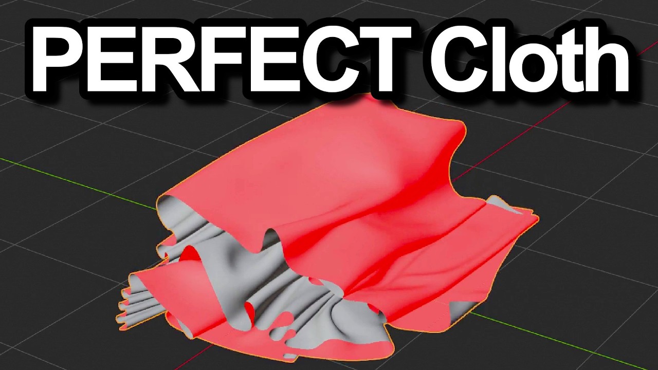
Here are some highlights:
We maintain a full docs site with workflow guides and recorded walkthroughs for the add-on:

Here are a couple of screenshots of the add-on running inside Blender:
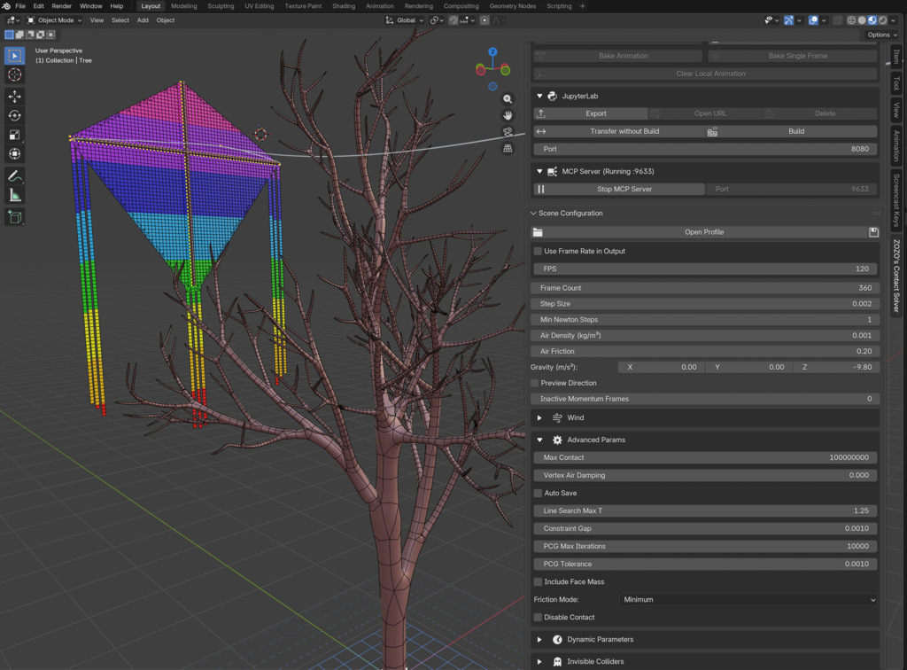 | 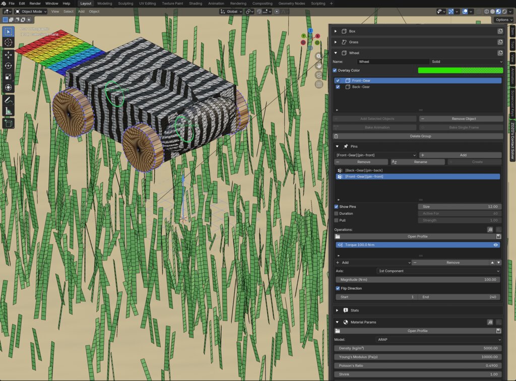 |
| Kite scene set up in Blender. (full-size) | Zebra scene set up in Blender. (full-size) |
We expose all of the add-on's tools through an MCP server, so any LLM (Claude, Codex, etc.) can drive the whole pipeline from a natural language prompt. Scene building, parameter tweaks, and running the simulation all happen without UI clicks. Here are two examples:
 |  |
| Codex (left) driving Blender (right) through the add-on's MCP server. | A prompt: drape a sheet over a sphere and make an animation video mp4 render 300 frames. |
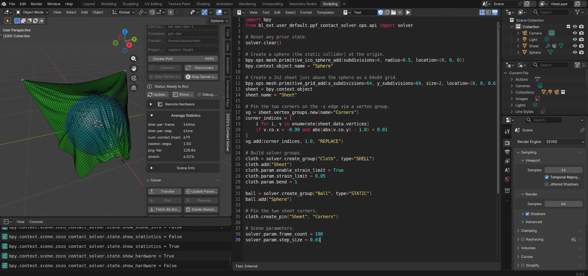
You can also drive the entire pipeline from a Python script inside Blender's scripting editor. This is handy for procedural scene setup and batch variant generation. Below is a full example that drapes a sheet over a sphere:
import addon_utils
import importlib
import bpy

# Look up the add-on module under whichever extension repository Blender
# installed it into and grab the public solver API.
addon = next(m for m in addon_utils.modules() if m.__name__.endswith(".ppf_contact_solver"))
solver = importlib.import_module(f"{addon.__name__}.ops.api").solver

# Reset any prior state.
solver.clear()

# Create a sphere (the static collider) at the origin.
bpy.ops.mesh.primitive_ico_sphere_add(subdivisions=4, radius=0.5, location=(0, 0, 0))
bpy.context.object.name = "Sphere"

# Create a 2x2 sheet just above the sphere as a 64x64 grid.
bpy.ops.mesh.primitive_grid_add(x_subdivisions=64, y_subdivisions=64, size=2, location=(0, 0, 0.6))
sheet = bpy.context.object
sheet.name = "Sheet"

# Pin the two corners on the -x edge via a vertex group.
vg = sheet.vertex_groups.new(name="Corners")
corner_indices = [
    i for i, v in enumerate(sheet.data.vertices)
    if v.co.x < -0.99 and abs(abs(v.co.y) - 1.0) < 0.01
]
vg.add(corner_indices, 1.0, "REPLACE")

# Build solver groups.
cloth = solver.create_group("Cloth", type="SHELL")
cloth.add("Sheet")
cloth.param.enable_strain_limit = True
cloth.param.strain_limit_percent = 5.0
cloth.param.bend = 1

ball = solver.create_group("Ball", type="STATIC")
ball.add("Sphere")

# Pin the two sheet corners.
cloth.create_pin("Sheet", "Corners")

# Scene parameters.
solver.param.frame_count = 100
solver.param.step_size = 0.01
Here's how the script runs inside Blender (full-size):
For the full solver.* surface, see the Blender Python API guide.
Our add-on ships UI catalogs for 日本語, 简体中文, and 한국어, selectable from Edit → Preferences → Interface → Translation. narznarznarz polished our Korean catalog to match Blender's own Korean terminology (Discussion):
ko_KR.json by narznarznarzTo install, download it (keep the name ko_KR.json) and overwrite the ko_KR.json in the installed add-on's i18n directory, which this prints in Blender's Python Console:
import addon_utils, os
addon = next(m for m in addon_utils.modules() if m.__name__.endswith(".ppf_contact_solver"))
print(os.path.join(os.path.dirname(addon.__file__), "i18n"))
Then restart Blender. Updating the add-on restores our catalog, so re-apply it after an update.
Our frontend is accessible through a browser using our built-in JupyterLab interface. All is set up when you open it for the first time. Results can be interactively viewed through the browser and exported as needed. Our Python interface is designed with the following principles in mind:

.triangulate() and .tetrahedralize() calls to keep everything in-pipeline, allowing users to skip explicit mesh exports to 3D/CAD software.from frontend import App.Here's an example of draping five sheets over a sphere with two corners pinned. We have more examples in the examples directory. Please take a look! 👀
# import our frontend
from frontend import App

# make an app
app = App.create("drape")

# create a square mesh resolution 128 spanning the xz plane
V, F = app.mesh.square(res=128, ex=[1, 0, 0], ey=[0, 0, 1])

# add to the asset and name it "sheet"
app.asset.add.tri("sheet", V, F)

# create an icosphere mesh radius 0.5
V, F = app.mesh.icosphere(r=0.5, subdiv_count=4)

# add to the asset and name it "sphere"
app.asset.add.tri("sphere", V, F)

# create a scene
scene = app.scene.create()

# define gap between sheets
gap = 0.01

for i in range(5):

    # add the sheet asset to the scene with an vertical offset
    obj = scene.add("sheet").at(0, gap * i, 0)

    # pick two corners
    corner = obj.grab([1, 0, -1]) + obj.grab([-1, 0, -1])

    # pin the corners
    obj.pin(corner)

    # set the strict limit on maximum strain to 5% per triangle
    obj.param.set("strain-limit", 0.05)

# add a sphere mesh at a lower position with jitter and set it static collider
scene.add("sphere").at(0, -0.5 - gap, 0).jitter().pin()

# compile the scene and report stats
scene = scene.build().report()

# preview the initial scene, shows image left
scene.preview()

# create a new session with the compiled scene
session = app.session.create(scene)

# set session params
session.param.set("frames", 100).set("dt", 0.01)

# build this session
session = session.build()

# start the simulation and live-preview the results, shows image right
session.start().preview()

# also show streaming logs
session.stream()

# or interactively view the animation sequences
session.animate()

# export all simulated frames in (sequences of ply meshes + a video)
session.export.animation()
Full API documentation is available on our GitHub Pages. The major APIs are documented using docstrings and compiled with Sphinx
We have also included jupyter-lsp to provide interactive linting assistance and display docstrings as you type. See this video (Video) for an example.
The behaviors can be changed through the settings.
A list of parameters used in param.set(key,value) is documented here: (Simulation Parameters) (Material Parameters).
⚠️ Please note that our Python APIs are subject to breaking changes as this repository undergoes frequent iterations. If you need APIs to be fixed, please fork.
Logs for the simulation can also be queried through our Python APIs. Here's an example of how to get a list of recorded logs, fetch them, and compute the average.
# get a list of log names
logs = session.get.log.names()
print(logs)
assert "time-per-frame" in logs
assert "newton-steps" in logs

# get a list of time per video frame
msec_per_video = session.get.log.numbers("time-per-frame")

# compute the average time per video frame
print("avg per frame:", sum([n for _, n in msec_per_video]) / len(msec_per_video))

# get a list of newton steps
newton_steps = session.get.log.numbers("newton-steps")

# compute the average of consumed newton steps
print("avg newton steps:", sum([n for _, n in newton_steps]) / len(newton_steps))

# Last 8 lines. Omit for everything.
print("==== log stream ====")
for line in session.get.log.stdout(n_lines=8):
    print(line)
Below are some representatives.
vid_time refers to the video time in seconds and is recorded as float.
ms refers to the consumed simulation time in milliseconds recorded as int.
vid_frame is the video frame count recorded as int.
| Name | Description | Format |
|---|---|---|
| time-per-frame | Time per video frame | list[(vid_frame,ms)] |
| matrix-assembly | Matrix assembly time | list[(vid_time,ms)] |
| pcg-linsolve | Linear system solve time | list[(vid_time,ms)] |
| line-search | Line search time | list[(vid_time,ms)] |
| time-per-step | Time per step | list[(vid_time,ms)] |
| newton-steps | Newton iterations per step | list[(vid_time,count)] |
| num-contact | Contact count | list[(vid_time,count)] |
| max-sigma | Max stretch | list(vid_time,float) |
The full list of log names and their descriptions is documented here: (GitHub Pages).
Note that some entries have multiple records at the same video time. This occurs because the same operation is executed multiple times within a single step during the inner Newton's iterations. For example, the linear system solve is performed at each Newton's step, so if multiple Newton's steps are executed, multiple linear system solve times appear in the record at the same video time.
If you would like to retrieve the raw log stream, you can do so by
# Last 8 lines. Omit for everything.
for line in session.get.log.stdout(n_lines=8):
    print(line)
This will output something like:
* dt: 1.000e-03
* max_sigma: 1.045e+00
* avg_sigma: 1.030e+00
------ newton step 1 ------
   ====== contact_matrix_assembly ======
   > dry_pass...0 msec
   > rebuild...7 msec
   > fillin_pass...0 msec
If you would like to read stderr, you can do so using session.get.log.stderr() (if it exists).
This returns list[str].
All the log files are updated in real-time and can be fetched right after the simulation starts; you don't have to wait until it finishes.

These scenes are all built with our add-on. The simulation itself runs on a remote solver, or directly on your local machine if you have a modern NVIDIA GPU on Windows or Linux, or an Apple silicon Mac.
You set the geometry, constraints, and parameters from Blender's UI, and the saved .blend carries everything the add-on needs.
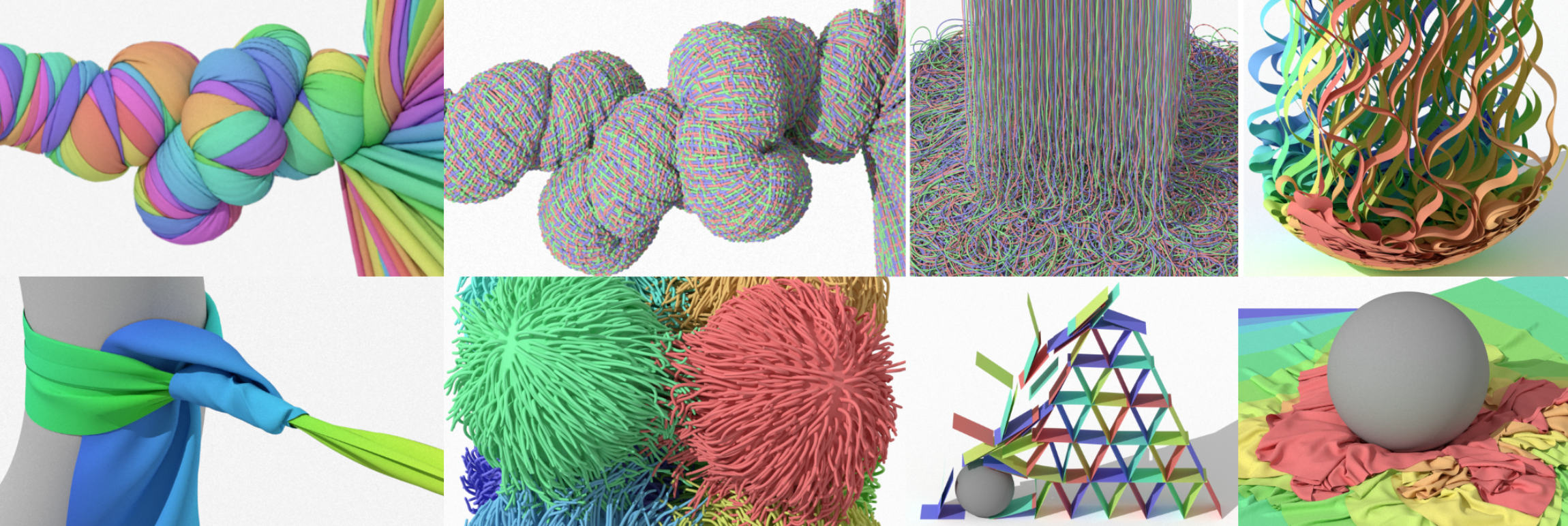
| kite.blend (Video) | crumple.blend (Video) | puff.blend (Video) |
 |  |  |
| press.blend (Video) | zebra.blend (Video) | curtain.blend (Video) |
 |  |  |
The simulated portion (objects, groups, pins, and solver parameters) is generated by a script you drop into Blender's Scripting editor. Cameras, lighting, and any non-simulated props are still set up in Blender's UI. Each script is linked above its thumbnail.
All these examples run on our Python frontend through JupyterLab. Click any notebook to see how the scene is built, or click the video link to watch the result.
Below is a table summarizing the estimated costs for running our examples on a NVIDIA L4 instance g6.2xlarge at Amazon Web Services US regions (us-east-1 and us-east-2).
| Example | Cost | Time | #Frame | #Vert | #Face | #Tet | #Rod | Max Strain |
|---|---|---|---|---|---|---|---|---|
| trapped | $0.08 | 4.66m | 300 | 135.4K | 216.5K | 416.5K | N/A | N/A |
| twist | $0.37 | 22.4m | 430 | 204.0K | 406.8K | N/A | N/A | N/A |
| stack | $0.28 | 16.5m | 120 | 167.4K | 327.7K | 12.7K | N/A | 5% |
| trampoline | $0.13 | 8.03m | 60 | 36.4K | 56.8K | 78.2K | N/A | 1% |
| needle | $0.20 | 11.7m | 120 | 86.8K | 169.0K | 12.7K | N/A | 5% |
| cards | $0.08 | 4.54m | 180 | 9.4K | 13.9K | 6.0K | N/A | N/A |
| domino | $0.06 | 3.38m | 250 | 0.5K | 0.8K | 0.3K | N/A | N/A |
| drape | $0.04 | 2.67m | 100 | 81.9K | 161.3K | N/A | N/A | 5% |
| curtain | $0.18 | 10.6m | 300 | 64.0K | 124.2K | N/A | N/A | 5% |
| friction | $0.16 | 9.63m | 850 | 3.3K | 4.3K | 12.0K | N/A | N/A |
| hang | $0.14 | 8.54m | 200 | 16.4K | 32.3K | N/A | N/A | 1% |
| belt | $0.08 | 5.09m | 200 | 12.3K | 23.3K | N/A | N/A | 5% |
| codim | $0.11 | 6.80m | 240 | 61.6K | 73.6K | 234.5K | 1.3K | N/A |
| fishingknot | $0.08 | 4.89m | 350 | 19.6K | 36.9K | N/A | N/A | 5% |
| fitting | $0.02 | 1.26m | 240 | 28.5K | 54.9K | N/A | N/A | 10% |
| noodle | $0.09 | 5.25m | 240 | 116.3K | N/A | N/A | 116.2K | N/A |
| ribbon | $0.25 | 14.8m | 480 | 35.6K | 53.0K | 12.6K | N/A | N/A |
| woven | $0.39 | 23.2m | 450 | 115.6K | N/A | N/A | 115.4K | N/A |
| yarn | $0.01 | 0.25m | 120 | 28.6K | N/A | N/A | 28.5K | N/A |
| roller | $0.04 | 2.64m | 180 | 6.2K | 11.0K | 7.1K | N/A | N/A |
Large scale examples are run on a vast.ai instance with an RTX 4090. These examples are not included in GitHub Action tests since they can take days to finish.
| Example | Commit | #Vert | #Face | #Rod | #Contact | #Frame | Time/Frame |
|---|---|---|---|---|---|---|---|
| large-twist | cbafbd2 | 3.2M | 6.4M | N/A | 56.7M | 2,000 | 46.4s |
| large-five-twist | 6ab6984 | 8.2M | 16.4M | N/A | 184.1M | 2,413 | 144.5s |
| large-woven | 4c07b83 | 2.7M | N/A | 2.7M | 8.9M | 946 | 436.8s |
📝 Large scale examples take a very long time, and it's easy to lose connection or close the browser. Our frontend lets you close and reopen it at your convenience. Just recover your session after you reconnect. Here's an example cell how to recover:
# In case you shutdown the server (or kernel) and still want
# to restart, do this.
# Do not run other cells used to create this scene.
# You can also recover this way if you closed the browser.
# Just directly run this in a new cell or in a new notebook.

from frontend import App

# recover the session
session = App.recover("app-name")

# resume if not currently running
if not App.busy():
    session.resume()

# preview the current state
session.preview()

# stream the logs
session.stream()
We implemented GitHub Actions that test all of our examples except for large scale ones, which take from days to weeks to finish. We perform explicit intersection checks at the end of each step, which raises an error if an intersection is detected. This ensures that all steps are confirmed to be penetration-free if tests pass. The runner types are described as follows:
This action builds the solver and runs a single headless example from start to finish on a freshly launched g6e.2xlarge AWS instance, so every run starts from a clean environment. 🌱
Like the Getting Started action, these build the solver and run the examples from start to finish on freshly launched g6e.2xlarge AWS instances, so every run starts from a clean environment.
Each example runs in parallel on its own instance, which reduces the total action time. 🌱
This action exercises our Blender add-on on Linux, Windows, and macOS in parallel. The Linux and Windows jobs run against the real CUDA solver on freshly launched g6e.2xlarge AWS instances, and the macOS job runs on a free GitHub-hosted runner that drives another such instance over the add-on's SSH connection. Blender 5.2.0 is installed from the official Blender Foundation mirror, and the add-on is installed as a Blender 5 extension. A headless test rig then runs the scenario registry covering add-on UI flows, sharded across the instances.
We generate zipped action artifacts for each run. These artifacts include:
Please note that these artifacts will be deleted after a month.
We know that you can't judge the reliability of contact resolution by simply watching a single success video example. To ensure greater transparency, we implemented GitHub Actions to run many of our examples via automated GitHub Actions, not just once, but 10 times in a row for both Linux and Windows. This means that a single failure out of 10 tests is considered a failure of the entire test suite! Also, we apply small jitters to the position of objects in the scene, so at each run, the scene is slightly different.


Running our solver on the cloud has a few practical advantages:
Below, we describe how to deploy our solver on major cloud services. These instructions are up to date as of late 2024 and are subject to change.
⚠️ For all the services below, don't forget to delete the instance after use, or you'll be charged for nothing. 💸
ssh -L 8080:localhost:8080 root@<host> -p <port>, then open http://localhost:8080 in your browser.fr-par-2L4-1-24G or GPU-3070-SUbuntu Jammy GPU OS 12Deep Learning Base AMI with Single CUDA (Ubuntu 22.04)g6.2xlarge (Recommended)GPUs. We recommend the GPU type NVIDIA L4 because it's affordable and accessible, as it does not require a high quota. You may select T4 instead for testing purposes.Enable Virtual Workstation (NVIDIA GRID).g2-standard-8.Deep Learning VM with CUDA 12.4 M129 and set the disk size to 50GB.us-central1 (Iowa) and $1.00 per hour in asia-east1 (Taiwan).8080 is reserved by the OS image. Set $MY_WEB_PORT to 8888. When connecting via gcloud, use the following format: gcloud compute ssh --zone "xxxx" "instance-name" -- -L 8080:localhost:8888.Alongside our official Blender add-on, the following community add-ons are also available:
Our work still needs many improvements, and our documentation and tutorial videos are not very sophisticated. The author would greatly appreciate it if you made your own tutorial videos, write-ups, or blog posts about the solver, and posted them online on YouTube, your blog, social media, or anywhere else.
If you post about it on X.com, please consider using the #ZOZOContactSolver tag so the author and community users can find your work.
This project is released under the Apache License 2.0. In plain terms, you may use, modify, and redistribute the code in commercial products, including proprietary software, without paying royalties or open-sourcing your own code. You only need to preserve the license notice and the attribution required by the license.
If you build something on top of this solver, we would love to hear about it, but you are not obligated to disclose anything.
If you like, we suggest taking the whole source code apart and building your own solver tailored to your specific needs. With the recent advances in coding agents, this is very likely possible even without any expertise in physics or coding.
Once you build your own, you are free to publish it as your own project or commercialize it, as long as you follow the Apache License 2.0 terms described above.
You don't need to use this project as is. Customize it as you like!
We cannot accept pull requests directly, since that involves resolving copyright and licensing matters with ZOZO, Inc. Instead, please open an issue for bug reports and proposals, or fork the repository and share a reference implementation for us to review. Substantial contributions will be credited here.
Issues are triaged in batches by a single part-time maintainer (Ryoichi Ando) and labeled queued (seen), in-progress (started), or worked (answered at least once), so please be patient if a response takes a while.
When reporting an issue, please attach a .blend file that reproduces it if possible. Remove any copyrightable materials from the scene or replace them with openly licensed alternatives. Because GitHub does not support direct .blend uploads, compress the file into a ZIP archive (for example, scene.blend.zip) before attaching it.
Please do not submit any other copyrightable materials through Issues or Discussions. Thank you!
We have opened GitHub Discussions as a place for questions, ideas, and conversations about the solver. Feel free to drop by to ask questions, share your work, or chat with the community.
This project is owned by ZOZO, Inc. and maintained by Ryoichi Ando.
For bug reports or feature requests, please open an issue on GitHub. For usage questions, GitHub Discussions is the best place to ask. Either route is the fastest way to reach the author and keeps the conversation searchable for other users.
If you would prefer to reach out privately, you can also email the author at ryoichi.ando@zozo.com. Please do not send any copyrightable materials; anything of that kind will never be read by the author and will be deleted upon receipt.
If you used this project in a public piece of work, whether a paper, a production credit, or a personal project, the author would love to feature it here. A link to your article, project page, or website is all we need (rather than images or clips themselves, since hosting them here may run into licensing issues), and we will be happy to add it.
We employ Continuous Collision Detection (CCD), not Discrete Collision Detection (DCD). Our cubic barrier theoretically guarantees penetration-free contact by construction, not heuristics, only when a solution is found. A solution may not be found in extreme cases, for example:
In such extreme cases, as well as with bugs, the solver may crash, stall, or take nearly forever to find a solution. What we guarantee is that every step that succeeds is free of intersections.
An intersection checker confirms zero penetration after every successful run and every step in GitHub Actions, so no hidden intersections are left behind.
Examples include pinned panels driven through each other (#116) and cloth trapped in a self-intersecting character animation (#110). Stopping preserves the guarantee, while completing would silently accept penetration. Check the scene before reporting a bug.
| Question | Answer |
|---|---|
| Why did ZOZO, Inc. make this? | To accelerate our internal R&D. Please read this article from ZOZO, Inc. (Japanese): https://corp.zozo.com/topics/20241125-siggraphasia/ |
| Why is this very slow? | We use a very different physics that guarantees strain limiting (e.g., no stretching over 2%) and penetration-free. That costs a lot. Other popularized solvers (e.g., XPBD) are much faster, but we don't know how to satisfy the two guarantees with them. |
| This paper <XXX> is faster than yours! | We are aware of that, so we never claim the state-of-the-art performance. |
| Should we use it? | Honestly, not yet for serious use. We still have many bugs, and performance is too slow. A lot needs to be fixed and improved. We are on it. |
| I bumped into a bug. | We kindly ask you to report it via GitHub Issues. See Contributing for what to attach. |
| Is this better than <Your Favorite Product>? | Partly yes, partly no. ZOZO's Contact Solver is not a drop-in replacement for any commercial product. |
| So what is it good for? | See the Catalogue and the community YouTube videos. They show what we can do. |
| Why did you separate the backend communicator and the solver engine? I would prefer an all-in-one, single-click setup. | Our main target is cloud use, such as AWS, rather than running on a desktop computer. |
| Why did you make the setup this complicated? | For internal use reasons. For now, see the CGMatter YouTube video and our video tutorials. They are much cleaner. |
| I don't have GPUs. Can I use this? | Yes, all the features run on the CPU backend (or Metal on Apple silicon), but it does not scale to large-scale scenes. See Requirements. |
| Does it run on AMD and Apple silicon (Metal) GPUs? | Yes. See Requirements. |
| Is it really intersection-free? | If the simulation does not crash or stall, yes, it is exactly 100% intersection-free. We never promise that the simulation will not crash or stall. |
| Why should I believe you? | We perform explicit intersection checks at the end of every step. See How Do We Promise No Intersections?. |
| Overhyped? | Many people seem to think it runs in real time and are disappointed to learn that it does not. We have laid out clear limitations in Gentle Disclaimer and Limitations. |
| I got an intersection error. Why is that? | In some situations, penetration is structurally unavoidable. See Intersection Errors Can Also Indicate an Impossible Setup. |
| Doesn't LLM-assisted coding compromise reliability? | The author can neither write code faster than an LLM nor write smarter or more polished code than the latest LLM models. We run extensive tests through GitHub Actions to assure reliability as best we can. |
| But LLMs can make mistakes. | The author makes more mistakes. |
| Did you write everything using AI? | We try to let AI handle what it is reliable at. However, Claude Code did not exist when our TOG paper (2024) was published, and until it did, we wrote everything ourselves, except for completions suggested by Copilot. We know what we are doing. |
| How large is your team? | A single person (Ryoichi Ando). Security reviews and legal checks are done by responsible teams at ZOZO, Inc. |
| This README is TL;DR. | Just watch the CGMatter YouTube video. That's the best starting point. |
The author thanks ZOZO, Inc. for permitting the release of the code and the team members for assisting with the internal paperwork for this project. The author expresses gratitude to GitHub community users for their feedback in Issues and Discussions, which has greatly helped track down and fix bugs, and for proposing feature requests that have strengthened this solver. The author also thanks everyone who has shared videos featuring this solver on YouTube, helping introduce it to a wider audience. This repository is owned by ZOZO, Inc.
(top 24 of 45)
335 followers · starred May 2026
1,859 followers · starred Oct 2025
485 followers · starred Jul 2026
717 followers · starred May 2026
A contact solver for physics-based simulations involving 👚 shells, 🪵 solids, 🪢 rods, 🧱 rigid bodies and ⏳ sand.
Python
4,550
462 commits
updated Oct 8, 2026
A contact solver for physics-based simulations involving 👚 shells, 🪵 solids, 🪢 rods, 🧱 rigid bodies and ⏳ sand. Started as an in-house physics engine at ZOZO, Inc., the largest fashion e-commerce company in Japan, and now evolving with the community. All open-source.
🤖 LLM Transparency: We highly respect that readers expect to hear the author's original voice and tone, which we work to retain throughout. Our use of LLMs is clarified in (Markdown).
If you simply want to use this through Blender, watch this CGMatter YouTube video. The release page is here. Our video tutorials page is here.
🎨 Simulate remotely from our Blender add-on (screenshots taken on macOS; you can also run locally on a modern NVIDIA GPU on Windows or Linux, or on an Apple silicon Mac)
https://github.com/user-attachments/assets/f266111e-7380-428b-8a3c-25eac4f039e5
🚀 Or run it locally: ./ppf-contact-solver (macOS/Linux), double click start.bat (Windows), or a Docker command (Linux/Windows)
🌐 Click the URL and explore our examples
📚 For the complete change history, see articles/changes.md.
https://github.com/user-attachments/assets/ac104255-604e-4890-9fb1-59732f004f0a
The main branch is undergoing frequent updates and will deviate from the paper.
To retain consistency with the paper, we have created a new branch sigasia-2024.
ghcr.io/st-tech/ppf-contact-solver-compiled-sigasia-2024:latest of this branch.A GPU is recommended, but not required. The right backend is picked for you when a run starts.
| Hardware | Backend | Runs on | Good to know |
|---|---|---|---|
| 🟩 NVIDIA GPU | CUDA 12.8+ | Linux (x86_64, arm64), Windows (x86_64) | RTX 4090 / 5090 for large scenes; 3090 / 4070 / 5070 for small to medium ones |
| 🟥 AMD GPU | ROCm | Linux (x86_64), Windows (x86_64) | gfx9 through gfx12 |
| 🍎 Apple silicon | Metal | macOS | M1 / A14 generation or newer |
| 💻 Any CPU | CPU (x86_64, arm64) | macOS, Windows, Linux | SIMD-optimized using AVX2 and NEON instructions |
You will also need:
Whether you plan to use the Blender add-on or the JupyterLab interface, the solver engine itself must first be deployed. The steps below apply to both.
⚠️ Do not run
warmup.pylocally. If you do, you are very likely to hit failures and find it difficult to cleanup.
🤔 If you are cautious, you can review the build workflow to verify safety yourself. We try to maximize transparency; we never build locally and upload.
For Apple silicon Macs, a self-contained folder carrying the Metal and CPU backends. No Python, Homebrew, or Xcode installation is needed, and nothing is installed outside the folder.
./ppf-contact-solverJupyterLab frontend will auto-start. You should be able to access it at http://localhost:8080.
Keep the terminal window open; Ctrl+C shuts it down.
For Windows 10/11 users, a self-contained executable (several hundred MB) is available. No Python, Docker, or CUDA Toolkit installation is needed. All should simply work out of the box (Video). The x86_64 archive carries the CUDA, ROCm, and CPU backends, so one download serves an NVIDIA machine and an AMD one, while a Windows on ARM machine runs the CPU backend.
start.batJupyterLab frontend will auto-start. You should be able to access it at http://localhost:8080.
A self-contained directory for x86_64 and aarch64 machines running glibc 2.28 or newer. The x86_64 archive carries the CUDA, ROCm, and CPU backends, and the aarch64 one carries CUDA and the CPU backend. No Python, CUDA Toolkit, or ROCm installation is needed.
./ppf-contact-solverJupyterLab frontend will auto-start. You should be able to access it at http://localhost:8080.
Keep the terminal window open; Ctrl+C shuts it down.
Install a NVIDIA driver (Link) on your host system and follow the instructions below specific to the operating system to get a Docker running:
| 🐧 Linux | 🪟 Windows |
|---|---|
Install the Docker engine from here (Link). Also, install the NVIDIA Container Toolkit (Link). Just to make sure that the Container Toolkit is loaded, run sudo service docker restart. | Install the Docker Desktop (Link). You may need to log out or reboot after the installation. After logging back in, launch Docker Desktop to ensure that Docker is running. |
Next, run the following command to start the container. If no edits are needed, just copy and paste:
$MY_WEB_PORT = 8080      # JupyterLab port on your side
$MY_BLENDER_PORT = 9090  # Solver port for the Blender add-on
$IMAGE_NAME = "ghcr.io/st-tech/ppf-contact-solver-compiled:latest"
docker run --rm -it `
  --name ppf-contact-solver `
  --gpus all `
  -p ${MY_WEB_PORT}:${MY_WEB_PORT} `
  -p ${MY_BLENDER_PORT}:${MY_BLENDER_PORT} `
  -e WEB_PORT=${MY_WEB_PORT} `
  $IMAGE_NAME # Image size ~1GB
MY_WEB_PORT=8080      # JupyterLab port on your side
MY_BLENDER_PORT=9090  # Solver port for the Blender add-on
IMAGE_NAME=ghcr.io/st-tech/ppf-contact-solver-compiled:latest
docker run --rm -it \
  --name ppf-contact-solver \
  --gpus all \
  -p ${MY_WEB_PORT}:${MY_WEB_PORT} \
  -p ${MY_BLENDER_PORT}:${MY_BLENDER_PORT} \
  -e WEB_PORT=${MY_WEB_PORT} \
  $IMAGE_NAME # Image size ~1GB
The image download shall be started. Our image is hosted on GitHub Container Registry (~1GB). JupyterLab will then auto-start. Eventually you should be seeing:
==== JupyterLab Launched! 🚀 ====
     http://localhost:8080
    Press Ctrl+C to shutdown
================================
Next, open your browser and navigate to http://localhost:8080. The port 8080 can change if you change the MY_WEB_PORT variable.
Keep your terminal window open.
Now you are ready to go! 🎉
To shut down the container, just press Ctrl+C in the terminal.
The container will be removed and all traces will be cleaned up. 🧹
If you wish to keep the container running in the background, replace
--rmwith-d. To shutdown the container and remove it, rundocker stop ppf-contact-solver && docker rm ppf-contact-solver.
If you wish to build the docker image from scratch, please refer to the cleaner installation guide (Markdown).
We provide two frontends: a Blender add-on and a JupyterLab interface. The Blender add-on lets you build scenes and run simulations entirely within Blender's UI, while JupyterLab lets you script everything in Python from your browser. Both communicate with the same solver engine, so pick whichever you like.
In both cases, you can interact with the simulator on your laptop while the actual simulation runs on a remote headless server over the internet. This means that you don't have to own NVIDIA hardware, but can rent it at vast.ai for less than $0.5 per hour. That said, if you do have a modern NVIDIA GPU on a local Windows or Linux machine, or an Apple silicon Mac, you can also run the solver directly on it. Actually, this (Video) was recorded on a vast.ai instance. The experience is good! 👍
Our Blender add-on aims to offer a familiar UI that best feels like everything works locally, but under the hood, it communicates with a remote server where all simulations run, and then the results are fetched back.
This provides a unique experience where users can leverage powerful remote GPUs while working seamlessly in their local Blender environment. Remarkably, our Blender add-on works even on macOS systems 😊, unlike other CUDA-based physics simulator add-ons that require local NVIDIA GPUs. More importantly, you can work on a laptop without worrying about draining the battery fast. 🔋
Follow this page How to Install to learn how to install the add-on. For a thorough walk through workflow, we refer to our documentation below:
🎬 Prefer video? CGMatter walks through the full setup in this video tutorial:
Here are some highlights:
We maintain a full docs site with workflow guides and recorded walkthroughs for the add-on:
Here are a couple of screenshots of the add-on running inside Blender:
| |
| Kite scene set up in Blender. (full-size) | Zebra scene set up in Blender. (full-size) |
We expose all of the add-on's tools through an MCP server, so any LLM (Claude, Codex, etc.) can drive the whole pipeline from a natural language prompt. Scene building, parameter tweaks, and running the simulation all happen without UI clicks. Here are two examples:
| |
| Codex (left) driving Blender (right) through the add-on's MCP server. | A prompt: drape a sheet over a sphere and make an animation video mp4 render 300 frames. |
You can also drive the entire pipeline from a Python script inside Blender's scripting editor. This is handy for procedural scene setup and batch variant generation. Below is a full example that drapes a sheet over a sphere:
import addon_utils
import importlib
import bpy

# Look up the add-on module under whichever extension repository Blender
# installed it into and grab the public solver API.
addon = next(m for m in addon_utils.modules() if m.__name__.endswith(".ppf_contact_solver"))
solver = importlib.import_module(f"{addon.__name__}.ops.api").solver

# Reset any prior state.
solver.clear()

# Create a sphere (the static collider) at the origin.
bpy.ops.mesh.primitive_ico_sphere_add(subdivisions=4, radius=0.5, location=(0, 0, 0))
bpy.context.object.name = "Sphere"

# Create a 2x2 sheet just above the sphere as a 64x64 grid.
bpy.ops.mesh.primitive_grid_add(x_subdivisions=64, y_subdivisions=64, size=2, location=(0, 0, 0.6))
sheet = bpy.context.object
sheet.name = "Sheet"

# Pin the two corners on the -x edge via a vertex group.
vg = sheet.vertex_groups.new(name="Corners")
corner_indices = [
    i for i, v in enumerate(sheet.data.vertices)
    if v.co.x < -0.99 and abs(abs(v.co.y) - 1.0) < 0.01
]
vg.add(corner_indices, 1.0, "REPLACE")

# Build solver groups.
cloth = solver.create_group("Cloth", type="SHELL")
cloth.add("Sheet")
cloth.param.enable_strain_limit = True
cloth.param.strain_limit_percent = 5.0
cloth.param.bend = 1

ball = solver.create_group("Ball", type="STATIC")
ball.add("Sphere")

# Pin the two sheet corners.
cloth.create_pin("Sheet", "Corners")

# Scene parameters.
solver.param.frame_count = 100
solver.param.step_size = 0.01
Here's how the script runs inside Blender (full-size):
For the full solver.* surface, see the Blender Python API guide.
Our add-on ships UI catalogs for 日本語, 简体中文, and 한국어, selectable from Edit → Preferences → Interface → Translation. narznarznarz polished our Korean catalog to match Blender's own Korean terminology (Discussion):
ko_KR.json by narznarznarzTo install, download it (keep the name ko_KR.json) and overwrite the ko_KR.json in the installed add-on's i18n directory, which this prints in Blender's Python Console:
import addon_utils, os
addon = next(m for m in addon_utils.modules() if m.__name__.endswith(".ppf_contact_solver"))
print(os.path.join(os.path.dirname(addon.__file__), "i18n"))
Then restart Blender. Updating the add-on restores our catalog, so re-apply it after an update.
Our frontend is accessible through a browser using our built-in JupyterLab interface. All is set up when you open it for the first time. Results can be interactively viewed through the browser and exported as needed. Our Python interface is designed with the following principles in mind:
.triangulate() and .tetrahedralize() calls to keep everything in-pipeline, allowing users to skip explicit mesh exports to 3D/CAD software.from frontend import App.Here's an example of draping five sheets over a sphere with two corners pinned. We have more examples in the examples directory. Please take a look! 👀
# import our frontend
from frontend import App

# make an app
app = App.create("drape")

# create a square mesh resolution 128 spanning the xz plane
V, F = app.mesh.square(res=128, ex=[1, 0, 0], ey=[0, 0, 1])

# add to the asset and name it "sheet"
app.asset.add.tri("sheet", V, F)

# create an icosphere mesh radius 0.5
V, F = app.mesh.icosphere(r=0.5, subdiv_count=4)

# add to the asset and name it "sphere"
app.asset.add.tri("sphere", V, F)

# create a scene
scene = app.scene.create()

# define gap between sheets
gap = 0.01

for i in range(5):

    # add the sheet asset to the scene with an vertical offset
    obj = scene.add("sheet").at(0, gap * i, 0)

    # pick two corners
    corner = obj.grab([1, 0, -1]) + obj.grab([-1, 0, -1])

    # pin the corners
    obj.pin(corner)

    # set the strict limit on maximum strain to 5% per triangle
    obj.param.set("strain-limit", 0.05)

# add a sphere mesh at a lower position with jitter and set it static collider
scene.add("sphere").at(0, -0.5 - gap, 0).jitter().pin()

# compile the scene and report stats
scene = scene.build().report()

# preview the initial scene, shows image left
scene.preview()

# create a new session with the compiled scene
session = app.session.create(scene)

# set session params
session.param.set("frames", 100).set("dt", 0.01)

# build this session
session = session.build()

# start the simulation and live-preview the results, shows image right
session.start().preview()

# also show streaming logs
session.stream()

# or interactively view the animation sequences
session.animate()

# export all simulated frames in (sequences of ply meshes + a video)
session.export.animation()
Full API documentation is available on our GitHub Pages. The major APIs are documented using docstrings and compiled with Sphinx
We have also included jupyter-lsp to provide interactive linting assistance and display docstrings as you type. See this video (Video) for an example.
The behaviors can be changed through the settings.
A list of parameters used in param.set(key,value) is documented here: (Simulation Parameters) (Material Parameters).
⚠️ Please note that our Python APIs are subject to breaking changes as this repository undergoes frequent iterations. If you need APIs to be fixed, please fork.
Logs for the simulation can also be queried through our Python APIs. Here's an example of how to get a list of recorded logs, fetch them, and compute the average.
# get a list of log names
logs = session.get.log.names()
print(logs)
assert "time-per-frame" in logs
assert "newton-steps" in logs

# get a list of time per video frame
msec_per_video = session.get.log.numbers("time-per-frame")

# compute the average time per video frame
print("avg per frame:", sum([n for _, n in msec_per_video]) / len(msec_per_video))

# get a list of newton steps
newton_steps = session.get.log.numbers("newton-steps")

# compute the average of consumed newton steps
print("avg newton steps:", sum([n for _, n in newton_steps]) / len(newton_steps))

# Last 8 lines. Omit for everything.
print("==== log stream ====")
for line in session.get.log.stdout(n_lines=8):
    print(line)
Below are some representatives.
vid_time refers to the video time in seconds and is recorded as float.
ms refers to the consumed simulation time in milliseconds recorded as int.
vid_frame is the video frame count recorded as int.
| Name | Description | Format |
|---|---|---|
| time-per-frame | Time per video frame | list[(vid_frame,ms)] |
| matrix-assembly | Matrix assembly time | list[(vid_time,ms)] |
| pcg-linsolve | Linear system solve time | list[(vid_time,ms)] |
| line-search | Line search time | list[(vid_time,ms)] |
| time-per-step | Time per step | list[(vid_time,ms)] |
| newton-steps | Newton iterations per step | list[(vid_time,count)] |
| num-contact | Contact count | list[(vid_time,count)] |
| max-sigma | Max stretch | list(vid_time,float) |
The full list of log names and their descriptions is documented here: (GitHub Pages).
Note that some entries have multiple records at the same video time. This occurs because the same operation is executed multiple times within a single step during the inner Newton's iterations. For example, the linear system solve is performed at each Newton's step, so if multiple Newton's steps are executed, multiple linear system solve times appear in the record at the same video time.
If you would like to retrieve the raw log stream, you can do so by
# Last 8 lines. Omit for everything.
for line in session.get.log.stdout(n_lines=8):
    print(line)
This will output something like:
* dt: 1.000e-03
* max_sigma: 1.045e+00
* avg_sigma: 1.030e+00
------ newton step 1 ------
   ====== contact_matrix_assembly ======
   > dry_pass...0 msec
   > rebuild...7 msec
   > fillin_pass...0 msec
If you would like to read stderr, you can do so using session.get.log.stderr() (if it exists).
This returns list[str].
All the log files are updated in real-time and can be fetched right after the simulation starts; you don't have to wait until it finishes.
These scenes are all built with our add-on. The simulation itself runs on a remote solver, or directly on your local machine if you have a modern NVIDIA GPU on Windows or Linux, or an Apple silicon Mac.
You set the geometry, constraints, and parameters from Blender's UI, and the saved .blend carries everything the add-on needs.
| kite.blend (Video) | crumple.blend (Video) | puff.blend (Video) |
| | |
| press.blend (Video) | zebra.blend (Video) | curtain.blend (Video) |
| | |
The simulated portion (objects, groups, pins, and solver parameters) is generated by a script you drop into Blender's Scripting editor. Cameras, lighting, and any non-simulated props are still set up in Blender's UI. Each script is linked above its thumbnail.
All these examples run on our Python frontend through JupyterLab. Click any notebook to see how the scene is built, or click the video link to watch the result.
Below is a table summarizing the estimated costs for running our examples on a NVIDIA L4 instance g6.2xlarge at Amazon Web Services US regions (us-east-1 and us-east-2).
| Example | Cost | Time | #Frame | #Vert | #Face | #Tet | #Rod | Max Strain |
|---|---|---|---|---|---|---|---|---|
| trapped | $0.08 | 4.66m | 300 | 135.4K | 216.5K | 416.5K | N/A | N/A |
| twist | $0.37 | 22.4m | 430 | 204.0K | 406.8K | N/A | N/A | N/A |
| stack | $0.28 | 16.5m | 120 | 167.4K | 327.7K | 12.7K | N/A | 5% |
| trampoline | $0.13 | 8.03m | 60 | 36.4K | 56.8K | 78.2K | N/A | 1% |
| needle | $0.20 | 11.7m | 120 | 86.8K | 169.0K | 12.7K | N/A | 5% |
| cards | $0.08 | 4.54m | 180 | 9.4K | 13.9K | 6.0K | N/A | N/A |
| domino | $0.06 | 3.38m | 250 | 0.5K | 0.8K | 0.3K | N/A | N/A |
| drape | $0.04 | 2.67m | 100 | 81.9K | 161.3K | N/A | N/A | 5% |
| curtain | $0.18 | 10.6m | 300 | 64.0K | 124.2K | N/A | N/A | 5% |
| friction | $0.16 | 9.63m | 850 | 3.3K | 4.3K | 12.0K | N/A | N/A |
| hang | $0.14 | 8.54m | 200 | 16.4K | 32.3K | N/A | N/A | 1% |
| belt | $0.08 | 5.09m | 200 | 12.3K | 23.3K | N/A | N/A | 5% |
| codim | $0.11 | 6.80m | 240 | 61.6K | 73.6K | 234.5K | 1.3K | N/A |
| fishingknot | $0.08 | 4.89m | 350 | 19.6K | 36.9K | N/A | N/A | 5% |
| fitting | $0.02 | 1.26m | 240 | 28.5K | 54.9K | N/A | N/A | 10% |
| noodle | $0.09 | 5.25m | 240 | 116.3K | N/A | N/A | 116.2K | N/A |
| ribbon | $0.25 | 14.8m | 480 | 35.6K | 53.0K | 12.6K | N/A | N/A |
| woven | $0.39 | 23.2m | 450 | 115.6K | N/A | N/A | 115.4K | N/A |
| yarn | $0.01 | 0.25m | 120 | 28.6K | N/A | N/A | 28.5K | N/A |
| roller | $0.04 | 2.64m | 180 | 6.2K | 11.0K | 7.1K | N/A | N/A |
Large scale examples are run on a vast.ai instance with an RTX 4090. These examples are not included in GitHub Action tests since they can take days to finish.
| Example | Commit | #Vert | #Face | #Rod | #Contact | #Frame | Time/Frame |
|---|---|---|---|---|---|---|---|
| large-twist | cbafbd2 | 3.2M | 6.4M | N/A | 56.7M | 2,000 | 46.4s |
| large-five-twist | 6ab6984 | 8.2M | 16.4M | N/A | 184.1M | 2,413 | 144.5s |
| large-woven | 4c07b83 | 2.7M | N/A | 2.7M | 8.9M | 946 | 436.8s |
📝 Large scale examples take a very long time, and it's easy to lose connection or close the browser. Our frontend lets you close and reopen it at your convenience. Just recover your session after you reconnect. Here's an example cell how to recover:
# In case you shutdown the server (or kernel) and still want
# to restart, do this.
# Do not run other cells used to create this scene.
# You can also recover this way if you closed the browser.
# Just directly run this in a new cell or in a new notebook.

from frontend import App

# recover the session
session = App.recover("app-name")

# resume if not currently running
if not App.busy():
    session.resume()

# preview the current state
session.preview()

# stream the logs
session.stream()
We implemented GitHub Actions that test all of our examples except for large scale ones, which take from days to weeks to finish. We perform explicit intersection checks at the end of each step, which raises an error if an intersection is detected. This ensures that all steps are confirmed to be penetration-free if tests pass. The runner types are described as follows:
This action builds the solver and runs a single headless example from start to finish on a freshly launched g6e.2xlarge AWS instance, so every run starts from a clean environment. 🌱
Like the Getting Started action, these build the solver and run the examples from start to finish on freshly launched g6e.2xlarge AWS instances, so every run starts from a clean environment.
Each example runs in parallel on its own instance, which reduces the total action time. 🌱
This action exercises our Blender add-on on Linux, Windows, and macOS in parallel. The Linux and Windows jobs run against the real CUDA solver on freshly launched g6e.2xlarge AWS instances, and the macOS job runs on a free GitHub-hosted runner that drives another such instance over the add-on's SSH connection. Blender 5.2.0 is installed from the official Blender Foundation mirror, and the add-on is installed as a Blender 5 extension. A headless test rig then runs the scenario registry covering add-on UI flows, sharded across the instances.
We generate zipped action artifacts for each run. These artifacts include:
Please note that these artifacts will be deleted after a month.
We know that you can't judge the reliability of contact resolution by simply watching a single success video example. To ensure greater transparency, we implemented GitHub Actions to run many of our examples via automated GitHub Actions, not just once, but 10 times in a row for both Linux and Windows. This means that a single failure out of 10 tests is considered a failure of the entire test suite! Also, we apply small jitters to the position of objects in the scene, so at each run, the scene is slightly different.
Running our solver on the cloud has a few practical advantages:
Below, we describe how to deploy our solver on major cloud services. These instructions are up to date as of late 2024 and are subject to change.
⚠️ For all the services below, don't forget to delete the instance after use, or you'll be charged for nothing. 💸
ssh -L 8080:localhost:8080 root@<host> -p <port>, then open http://localhost:8080 in your browser.fr-par-2L4-1-24G or GPU-3070-SUbuntu Jammy GPU OS 12Deep Learning Base AMI with Single CUDA (Ubuntu 22.04)g6.2xlarge (Recommended)GPUs. We recommend the GPU type NVIDIA L4 because it's affordable and accessible, as it does not require a high quota. You may select T4 instead for testing purposes.Enable Virtual Workstation (NVIDIA GRID).g2-standard-8.Deep Learning VM with CUDA 12.4 M129 and set the disk size to 50GB.us-central1 (Iowa) and $1.00 per hour in asia-east1 (Taiwan).8080 is reserved by the OS image. Set $MY_WEB_PORT to 8888. When connecting via gcloud, use the following format: gcloud compute ssh --zone "xxxx" "instance-name" -- -L 8080:localhost:8888.Alongside our official Blender add-on, the following community add-ons are also available:
Our work still needs many improvements, and our documentation and tutorial videos are not very sophisticated. The author would greatly appreciate it if you made your own tutorial videos, write-ups, or blog posts about the solver, and posted them online on YouTube, your blog, social media, or anywhere else.
If you post about it on X.com, please consider using the #ZOZOContactSolver tag so the author and community users can find your work.
This project is released under the Apache License 2.0. In plain terms, you may use, modify, and redistribute the code in commercial products, including proprietary software, without paying royalties or open-sourcing your own code. You only need to preserve the license notice and the attribution required by the license.
If you build something on top of this solver, we would love to hear about it, but you are not obligated to disclose anything.
If you like, we suggest taking the whole source code apart and building your own solver tailored to your specific needs. With the recent advances in coding agents, this is very likely possible even without any expertise in physics or coding.
Once you build your own, you are free to publish it as your own project or commercialize it, as long as you follow the Apache License 2.0 terms described above.
You don't need to use this project as is. Customize it as you like!
We cannot accept pull requests directly, since that involves resolving copyright and licensing matters with ZOZO, Inc. Instead, please open an issue for bug reports and proposals, or fork the repository and share a reference implementation for us to review. Substantial contributions will be credited here.
Issues are triaged in batches by a single part-time maintainer (Ryoichi Ando) and labeled queued (seen), in-progress (started), or worked (answered at least once), so please be patient if a response takes a while.
When reporting an issue, please attach a .blend file that reproduces it if possible. Remove any copyrightable materials from the scene or replace them with openly licensed alternatives. Because GitHub does not support direct .blend uploads, compress the file into a ZIP archive (for example, scene.blend.zip) before attaching it.
Please do not submit any other copyrightable materials through Issues or Discussions. Thank you!
We have opened GitHub Discussions as a place for questions, ideas, and conversations about the solver. Feel free to drop by to ask questions, share your work, or chat with the community.
This project is owned by ZOZO, Inc. and maintained by Ryoichi Ando.
For bug reports or feature requests, please open an issue on GitHub. For usage questions, GitHub Discussions is the best place to ask. Either route is the fastest way to reach the author and keeps the conversation searchable for other users.
If you would prefer to reach out privately, you can also email the author at ryoichi.ando@zozo.com. Please do not send any copyrightable materials; anything of that kind will never be read by the author and will be deleted upon receipt.
If you used this project in a public piece of work, whether a paper, a production credit, or a personal project, the author would love to feature it here. A link to your article, project page, or website is all we need (rather than images or clips themselves, since hosting them here may run into licensing issues), and we will be happy to add it.
We employ Continuous Collision Detection (CCD), not Discrete Collision Detection (DCD). Our cubic barrier theoretically guarantees penetration-free contact by construction, not heuristics, only when a solution is found. A solution may not be found in extreme cases, for example:
In such extreme cases, as well as with bugs, the solver may crash, stall, or take nearly forever to find a solution. What we guarantee is that every step that succeeds is free of intersections.
An intersection checker confirms zero penetration after every successful run and every step in GitHub Actions, so no hidden intersections are left behind.
Examples include pinned panels driven through each other (#116) and cloth trapped in a self-intersecting character animation (#110). Stopping preserves the guarantee, while completing would silently accept penetration. Check the scene before reporting a bug.
| Question | Answer |
|---|---|
| Why did ZOZO, Inc. make this? | To accelerate our internal R&D. Please read this article from ZOZO, Inc. (Japanese): https://corp.zozo.com/topics/20241125-siggraphasia/ |
| Why is this very slow? | We use a very different physics that guarantees strain limiting (e.g., no stretching over 2%) and penetration-free. That costs a lot. Other popularized solvers (e.g., XPBD) are much faster, but we don't know how to satisfy the two guarantees with them. |
| This paper <XXX> is faster than yours! | We are aware of that, so we never claim the state-of-the-art performance. |
| Should we use it? | Honestly, not yet for serious use. We still have many bugs, and performance is too slow. A lot needs to be fixed and improved. We are on it. |
| I bumped into a bug. | We kindly ask you to report it via GitHub Issues. See Contributing for what to attach. |
| Is this better than <Your Favorite Product>? | Partly yes, partly no. ZOZO's Contact Solver is not a drop-in replacement for any commercial product. |
| So what is it good for? | See the Catalogue and the community YouTube videos. They show what we can do. |
| Why did you separate the backend communicator and the solver engine? I would prefer an all-in-one, single-click setup. | Our main target is cloud use, such as AWS, rather than running on a desktop computer. |
| Why did you make the setup this complicated? | For internal use reasons. For now, see the CGMatter YouTube video and our video tutorials. They are much cleaner. |
| I don't have GPUs. Can I use this? | Yes, all the features run on the CPU backend (or Metal on Apple silicon), but it does not scale to large-scale scenes. See Requirements. |
| Does it run on AMD and Apple silicon (Metal) GPUs? | Yes. See Requirements. |
| Is it really intersection-free? | If the simulation does not crash or stall, yes, it is exactly 100% intersection-free. We never promise that the simulation will not crash or stall. |
| Why should I believe you? | We perform explicit intersection checks at the end of every step. See How Do We Promise No Intersections?. |
| Overhyped? | Many people seem to think it runs in real time and are disappointed to learn that it does not. We have laid out clear limitations in Gentle Disclaimer and Limitations. |
| I got an intersection error. Why is that? | In some situations, penetration is structurally unavoidable. See Intersection Errors Can Also Indicate an Impossible Setup. |
| Doesn't LLM-assisted coding compromise reliability? | The author can neither write code faster than an LLM nor write smarter or more polished code than the latest LLM models. We run extensive tests through GitHub Actions to assure reliability as best we can. |
| But LLMs can make mistakes. | The author makes more mistakes. |
| Did you write everything using AI? | We try to let AI handle what it is reliable at. However, Claude Code did not exist when our TOG paper (2024) was published, and until it did, we wrote everything ourselves, except for completions suggested by Copilot. We know what we are doing. |
| How large is your team? | A single person (Ryoichi Ando). Security reviews and legal checks are done by responsible teams at ZOZO, Inc. |
| This README is TL;DR. | Just watch the CGMatter YouTube video. That's the best starting point. |
The author thanks ZOZO, Inc. for permitting the release of the code and the team members for assisting with the internal paperwork for this project. The author expresses gratitude to GitHub community users for their feedback in Issues and Discussions, which has greatly helped track down and fix bugs, and for proposing feature requests that have strengthened this solver. The author also thanks everyone who has shared videos featuring this solver on YouTube, helping introduce it to a wider audience. This repository is owned by ZOZO, Inc.
(top 24 of 45)
335 followers · starred May 2026
1,859 followers · starred Oct 2025
485 followers · starred Jul 2026
717 followers · starred May 2026