
Visualizes an LLM pipeline either as simulation or with a real LLM running in the browser. Created with Claude Code using Fable 5 and Superpowers.
0
stars
150
commits
TypeScript
primary language
Sep 3, 2026
updated
README
紬 Tsumugi — An LLM Pipeline Visualizer
Tsumugi (紬) is a traditional Japanese cloth woven from raw silk, prized for its rough, hand-spun texture. The name plays on the related verb 紡ぐ (tsumugu) — to spin, to weave: an LLM pipeline weaves its output token by token into text, each new thread pulled from the probability distribution the model spins over its vocabulary.
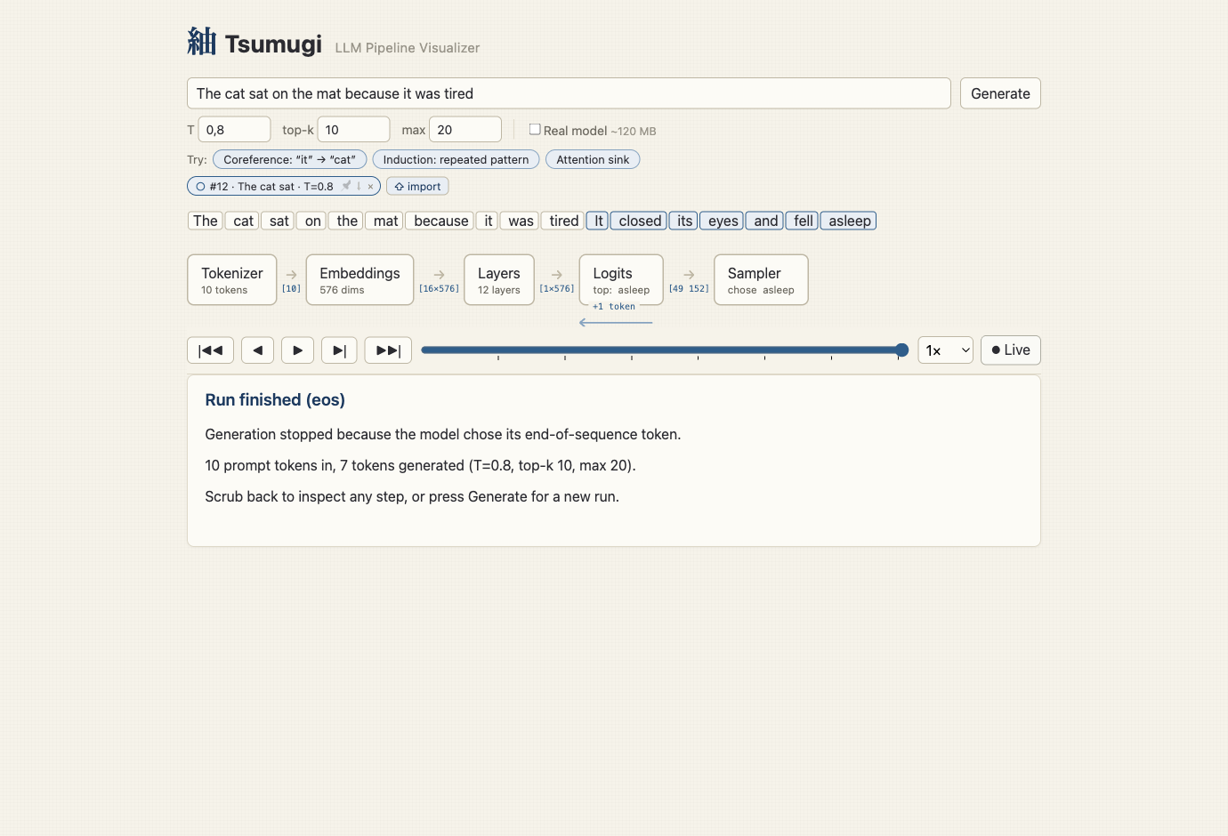
Tsumugi is a single-page app that visualizes how a prompt flows through an LLM's autoregressive generation loop — tokenize → embed → transformer layers → logits → softmax → sample → append → repeat. Built for developers and CS students who are comfortable with code but want to see what happens between typing a prompt and getting tokens back: tokenization, embeddings, per-layer activations, attention patterns, logits, probability distributions, and sampling.
You type a prompt, hit generate, and watch the pipeline stages light up as each token is produced — live, or one step at a time via manual playback controls.
Modes
- Simulated (default) — instant, fully offline, no model download. Uses a small real tokenizer (falling back to a built-in tokenizer if the Hugging Face tokenizer files can't be fetched) plus synthetic-but-realistic activations, logits, and sampling, so the pipeline stages behave the way a real model would without needing to run one.
- Real — runs an actual small model in-browser via
transformers.js, in a
Web Worker. It first tries a custom export of SmolLM2-135M-Instruct with
real per-layer attention outputs
(
saigyo-hoshi/smollm2-135m-attn-onnx, ~240 MB, downloaded once and cached): the Layers stage then shows measured attention heatmaps, with head roles (previous-token, attention-sink, induction, coreference) detected statistically from the weights on your prompt and labeled with their evidence scores. If that download fails it falls back to the stockHuggingFaceTB/SmolLM2-135M-Instructexport (~120 MB, schematic layers). Prefers WebGPU, falls back to WASM automatically.
One matrix, end to end — the residual stream
The pipeline stages look like separate machines, but there is only one
object flowing through the whole pipeline: a matrix X of shape
[seq_len × d_model] — one 576-dimensional vector per token position
(SmolLM2's numbers). This is the residual stream, and it answers every
"what happens between the stages" question:
- Embeddings → Layers: no hand-off, no conversion. The embedding stage's output — one vector per token, looked up from the embedding table — is layer 0's input, verbatim. The row strip in the Embeddings panel is a row of exactly the matrix that enters the first layer.
- Layer → Layer: each layer edits this matrix and passes it on —
and it edits by addition:
X ← X + attention(X), thenX ← X + MLP(X). Each token's vector accumulates refinements layer by layer, like a document going through thirty rounds of margin notes; the original embedding is still in there, with the corrections added on top. Inside a layer the jobs are strictly divided: attention is the only place information moves between token positions (the heatmap row for token i is the mixing recipe — row "it" = 65% "cat" means the vector at "it" gets a large dose of "cat"'s vector added in), while the MLP transforms each position's vector in isolation. - Layers → Logits: take only the last token's row of the final
matrix — one vector — normalize it, and multiply by the unembedding
matrix (
d_model × vocab, essentially the embedding table transposed). Each logit is literally a dot product: how similar is the final state of the last position to vocabulary token v's direction? That single matrix multiply is the Logits stage; softmax and sampling just turn the ~49k scores into a choice.
So the causal chain to the probabilities runs: attention weights decide
which vectors get blended into the last position's vector; the layers'
accumulated edits shape that vector; the logits read it out against
every vocabulary direction. The app shows this carrier explicitly — the
tensor-shape labels on the pipeline arrows (watch [10×576] narrow to
[1×576] before Logits), the layer-anatomy diagram in the Layers panel,
and the readout formula in the Logits panel.
The name of the app tells the same story: each token is a thread, attention decides which existing threads get twisted into the new one at each layer, and at the end the finished strand is held up against 49k reference threads to see which it resembles most.
What an embedding is — a lookup, then geometry
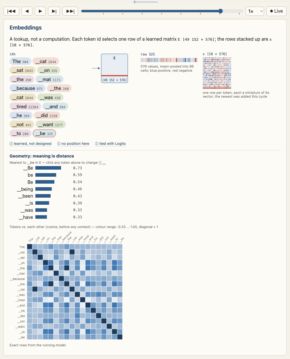
The Embeddings stage is the least mysterious step in the pipeline and the one most often hand-waved. The card makes two points, in order.
It is a lookup, not a computation. A token id selects one row of a
learned matrix E [49152 × 576]; the rows of the current sequence stacked
up are the residual stream x [n × 576] that the layers then edit. Click
any token chip to see its row. Three things worth knowing ride along as
hover notes: the rows are learned, not designed (nobody chose what
dimension 17 means); no position is added here — SmolLM2 applies rotary
position embeddings inside attention instead; and the same matrix is
reused at the Logits stage to read the answer back out (tied weights).
Meaning is distance. Similar tokens have similar rows. The card shows the eight nearest vocabulary neighbours of the selected token by cosine similarity, and a similarity matrix of the visible tokens against each other — what the model "knows" about these tokens before any context is applied, a useful contrast with the attention heatmaps one stage later.
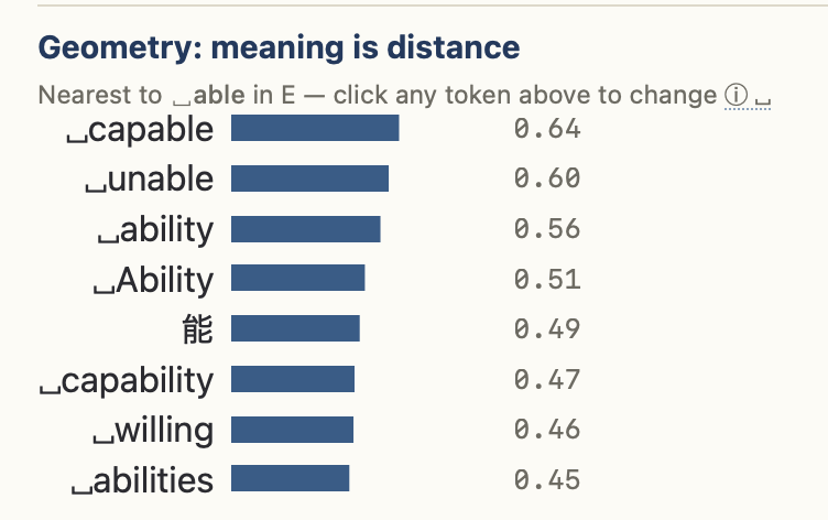
A specimen worth pausing on: the neighbours of able. Two lessons sit in
one list. First, distance knows no language — 能, the Chinese/Japanese
character for "can, ability", lands among the English ability words. It
has its own token because it is frequent enough in the training mix, and it
occurs in the same kinds of contexts as able and ability do, so training
pushed its row toward theirs; nobody told the model these are translations.
Second, unable is the second-closest neighbour: embedding similarity is
about shared contexts, not agreement in meaning. Antonyms are near-perfect
substitutes distributionally, so they sit side by side here, and the
negation has to be resolved later, by the layers. (The ␣ marks a leading
space — byte-level BPE keeps able and able as different tokens, and the
card shows both kinds side by side with their own similarities.)
In real mode the rows are the exact vectors from the running model (the
custom ONNX export exposes the embedding lookup as inputs_embeds). In
simulated mode, and for archived runs, they come from a small
vocabulary-geometry asset published next to the model on the Hugging Face
Hub: exact nearest neighbours computed offline over the full 576-dim table,
plus a PCA-64 int8 copy of every row for the similarity matrix — the caption
says which you are looking at.
Reading the attention heatmaps
The Layers stage shows attention heatmaps (simulated mode): a triangular grid per attention head, where row i shows how much the token at position i attends to each earlier token — every row sums to 100%. Mechanically these weights are the mixing recipe of the residual stream's attention step described above: they decide whose vectors get blended into each position. Real attention heads show strikingly legible patterns, and the simulated heads reproduce the canonical ones:
- Previous-token head — a bright diagonal stripe: this head mostly copies from the token just before. Local syntax.
- Attention sink — a bright first column: many heads dump most of their attention on the first token as a learned "do nothing" default. A famous, counterintuitive phenomenon invisible in any other view of the model.
- Induction head — with a repeated pattern in the prompt ("one two three one …"), attention jumps from a repeated token to whatever followed its previous occurrence. This is the circuit that interpretability research credits for in-context learning.
- Coreference — in "The cat sat on the mat because it was tired", watch the row for "it" attend back to "cat": the mechanism by which the model resolves what a pronoun refers to. SmolLM2-135M really has such a head (layer 13, head 8 — see the spike note); real mode finds it by asking which head's pronoun rows point most sharply at one earlier word, so check for yourself whether that word is the right referent.
The example chips under the prompt input load prompts crafted so these patterns visibly connect to the input; each head's caption says what to look for.
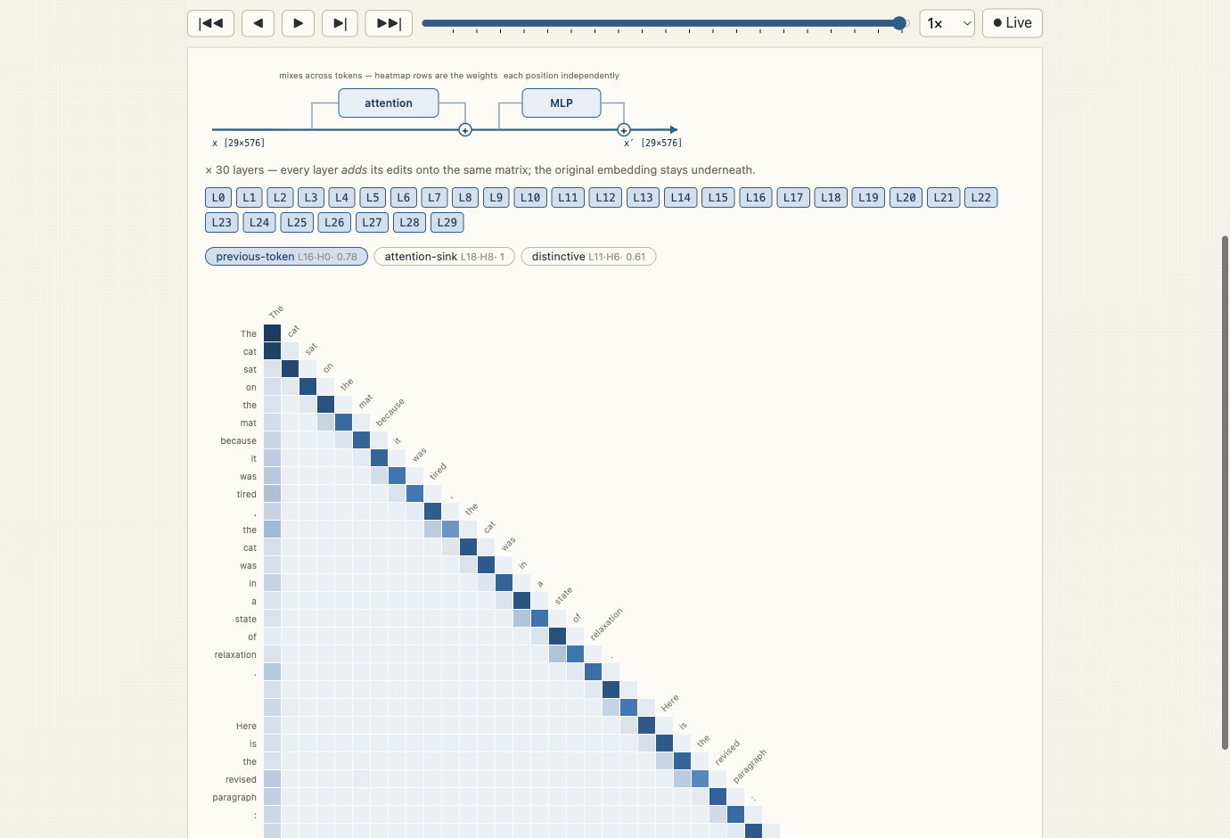
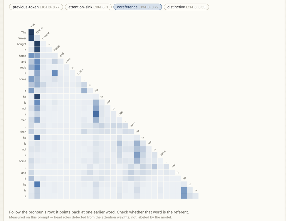
A specimen from the coreference head, on "The farmer bought a horse and
rode it home." and what the model wrote next ("If he is not a man, then he
is not a horse, and if he is a…"). Three things in one matrix. The prompt's
it row puts its weight on horse, the object, not on the subject — so
this is reference resolution, not just "look at the first noun". Every
generated he row goes back to farmer, the last one twenty tokens
away, with nothing in between competing. And between pronouns the head
chains: the rows for "is not a man" attend to the he just before them,
not to farmer, so the head tracks the most recent mention of the entity
and hops back to the noun only at the pronoun itself. Nobody labeled any of
this; the chip says coreference · 0.72 because that head's pronoun rows
are the most sharply pointed at one earlier content word of all 270 heads.
In real mode the detected chips are only the textbook specimens — the model has 30 layers × 9 heads = 270 heads in total, and Explore all heads opens a small-multiples grid of every one of them (mean-pooled thumbnails of the attention accumulated over the whole run, plus a per-layer average column). Sort by the detection scores to surface heads the chips missed, and click any thumbnail to pin its exact matrix into the viewer above.
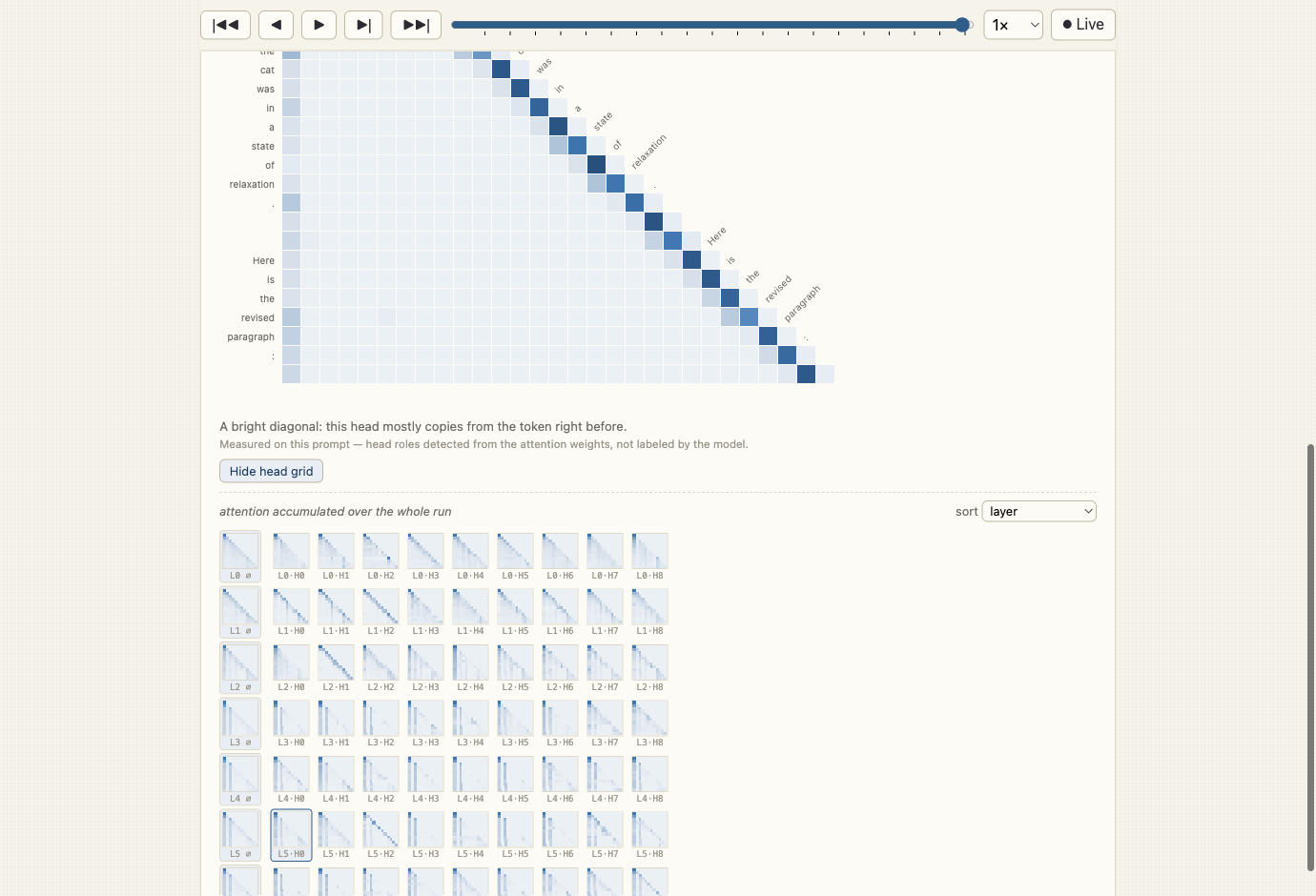
Two honest caveats. First, simulated mode's heatmaps are illustrative — deterministic, hand-shaped patterns of the kinds real models exhibit — while real mode shows measured weights from the custom model export (the footer under each heatmap says which you're looking at; head roles in real mode are detected from the weights, not labeled by the model). Second, even real attention weights are not explanations — they show what the mechanism computes, not why the model produced its output (Jain & Wallace, "Attention is not Explanation", 2019). Read them as "how information flows", never as "why the model answered X".
Comparing runs
Every completed run is kept on a run shelf under the prompt bar — generation stops being fire-and-forget. Runs survive page reloads (IndexedDB), the eight most recent are kept automatically, a pin (📌) protects a run from falling off, and any run can be exported as a JSON trace file and imported back later — on another machine, or into a bug report.
Select two runs (⇄ compare, then click a second chip) and everything below the shelf becomes a comparison view: both runs' parameters with differences highlighted, the two token streams aligned cycle by cycle, and — for runs with the same prompt — the fork marked: the first cycle where the two runs chose different tokens. Click any cycle (on the ruler or a word chip) to inspect it:
- Paired distributions — both runs' top-k probabilities at that cycle, with the sampled token marked. This is where sampling becomes visible: at the fork of two same-prompt runs the two distributions are often identical — same beliefs, different draw. Compare different temperatures on one prompt to watch the distribution itself change instead.
- Paired attention — the detected heads of both runs at that cycle, side by side. Where only one run promoted a head to a full-resolution snapshot, the other side falls back to its run-level thumbnail — an asymmetry that is itself informative (that run's content didn't activate the circuit strongly enough to win a chip).
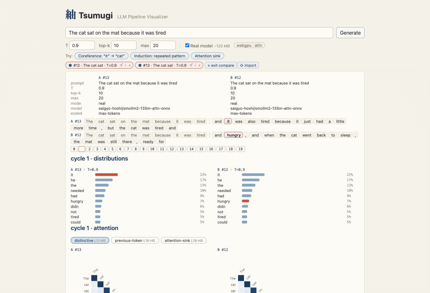
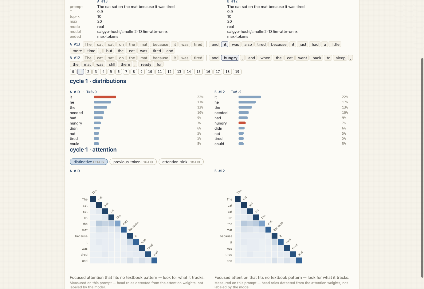
Comparison is pure trace inspection — no playback, no model in the loop — so it works identically for live, reloaded, and imported runs.
(The screenshots in this README are regenerated with npm run screenshots
— a headed-Chromium Playwright script that drives sim and real mode;
the first run downloads the model into a cached local profile.)
Running it
npm install
npm run dev
Then open the printed local URL (defaults to http://localhost:5173).
Testing
npm test      # unit tests (vitest)
npm run e2e   # end-to-end smoke test (playwright, chromium)
The end-to-end test drives the app in simulated mode only — it never
downloads or runs the real model, so it works fully offline and in CI. Run
npx playwright install chromium once before the first npm run e2e.
Docs
Ideas for future milestones are collected in
docs/BACKLOG.md.
The original design spec and implementation plan live under
docs/superpowers/:
specs/2026-08-26-llm-pipeline-visualizer-design.mdplans/2026-08-26-llm-pipeline-visualizer.mdspecs/2026-09-02-embeddings-explained-design.mdplans/2026-09-02-embeddings-explained.md
License
Contributors

150 commits
Similar repos


Languages
TypeScript
79.8%
Python
12.8%
CSS
5.5%
JavaScript
1.9%
Visualizes an LLM pipeline either as simulation or with a real LLM running in the browser. Created with Claude Code using Fable 5 and Superpowers.
0
stars
150
commits
TypeScript
primary language
Sep 3, 2026
updated
README
紬 Tsumugi — An LLM Pipeline Visualizer
Tsumugi (紬) is a traditional Japanese cloth woven from raw silk, prized for its rough, hand-spun texture. The name plays on the related verb 紡ぐ (tsumugu) — to spin, to weave: an LLM pipeline weaves its output token by token into text, each new thread pulled from the probability distribution the model spins over its vocabulary.
Tsumugi is a single-page app that visualizes how a prompt flows through an LLM's autoregressive generation loop — tokenize → embed → transformer layers → logits → softmax → sample → append → repeat. Built for developers and CS students who are comfortable with code but want to see what happens between typing a prompt and getting tokens back: tokenization, embeddings, per-layer activations, attention patterns, logits, probability distributions, and sampling.
You type a prompt, hit generate, and watch the pipeline stages light up as each token is produced — live, or one step at a time via manual playback controls.
Modes
- Simulated (default) — instant, fully offline, no model download. Uses a small real tokenizer (falling back to a built-in tokenizer if the Hugging Face tokenizer files can't be fetched) plus synthetic-but-realistic activations, logits, and sampling, so the pipeline stages behave the way a real model would without needing to run one.
- Real — runs an actual small model in-browser via
transformers.js, in a
Web Worker. It first tries a custom export of SmolLM2-135M-Instruct with
real per-layer attention outputs
(
saigyo-hoshi/smollm2-135m-attn-onnx, ~240 MB, downloaded once and cached): the Layers stage then shows measured attention heatmaps, with head roles (previous-token, attention-sink, induction, coreference) detected statistically from the weights on your prompt and labeled with their evidence scores. If that download fails it falls back to the stockHuggingFaceTB/SmolLM2-135M-Instructexport (~120 MB, schematic layers). Prefers WebGPU, falls back to WASM automatically.
One matrix, end to end — the residual stream
The pipeline stages look like separate machines, but there is only one
object flowing through the whole pipeline: a matrix X of shape
[seq_len × d_model] — one 576-dimensional vector per token position
(SmolLM2's numbers). This is the residual stream, and it answers every
"what happens between the stages" question:
- Embeddings → Layers: no hand-off, no conversion. The embedding stage's output — one vector per token, looked up from the embedding table — is layer 0's input, verbatim. The row strip in the Embeddings panel is a row of exactly the matrix that enters the first layer.
- Layer → Layer: each layer edits this matrix and passes it on —
and it edits by addition:
X ← X + attention(X), thenX ← X + MLP(X). Each token's vector accumulates refinements layer by layer, like a document going through thirty rounds of margin notes; the original embedding is still in there, with the corrections added on top. Inside a layer the jobs are strictly divided: attention is the only place information moves between token positions (the heatmap row for token i is the mixing recipe — row "it" = 65% "cat" means the vector at "it" gets a large dose of "cat"'s vector added in), while the MLP transforms each position's vector in isolation. - Layers → Logits: take only the last token's row of the final
matrix — one vector — normalize it, and multiply by the unembedding
matrix (
d_model × vocab, essentially the embedding table transposed). Each logit is literally a dot product: how similar is the final state of the last position to vocabulary token v's direction? That single matrix multiply is the Logits stage; softmax and sampling just turn the ~49k scores into a choice.
So the causal chain to the probabilities runs: attention weights decide
which vectors get blended into the last position's vector; the layers'
accumulated edits shape that vector; the logits read it out against
every vocabulary direction. The app shows this carrier explicitly — the
tensor-shape labels on the pipeline arrows (watch [10×576] narrow to
[1×576] before Logits), the layer-anatomy diagram in the Layers panel,
and the readout formula in the Logits panel.
The name of the app tells the same story: each token is a thread, attention decides which existing threads get twisted into the new one at each layer, and at the end the finished strand is held up against 49k reference threads to see which it resembles most.
What an embedding is — a lookup, then geometry
The Embeddings stage is the least mysterious step in the pipeline and the one most often hand-waved. The card makes two points, in order.
It is a lookup, not a computation. A token id selects one row of a
learned matrix E [49152 × 576]; the rows of the current sequence stacked
up are the residual stream x [n × 576] that the layers then edit. Click
any token chip to see its row. Three things worth knowing ride along as
hover notes: the rows are learned, not designed (nobody chose what
dimension 17 means); no position is added here — SmolLM2 applies rotary
position embeddings inside attention instead; and the same matrix is
reused at the Logits stage to read the answer back out (tied weights).
Meaning is distance. Similar tokens have similar rows. The card shows the eight nearest vocabulary neighbours of the selected token by cosine similarity, and a similarity matrix of the visible tokens against each other — what the model "knows" about these tokens before any context is applied, a useful contrast with the attention heatmaps one stage later.
A specimen worth pausing on: the neighbours of able. Two lessons sit in
one list. First, distance knows no language — 能, the Chinese/Japanese
character for "can, ability", lands among the English ability words. It
has its own token because it is frequent enough in the training mix, and it
occurs in the same kinds of contexts as able and ability do, so training
pushed its row toward theirs; nobody told the model these are translations.
Second, unable is the second-closest neighbour: embedding similarity is
about shared contexts, not agreement in meaning. Antonyms are near-perfect
substitutes distributionally, so they sit side by side here, and the
negation has to be resolved later, by the layers. (The ␣ marks a leading
space — byte-level BPE keeps able and able as different tokens, and the
card shows both kinds side by side with their own similarities.)
In real mode the rows are the exact vectors from the running model (the
custom ONNX export exposes the embedding lookup as inputs_embeds). In
simulated mode, and for archived runs, they come from a small
vocabulary-geometry asset published next to the model on the Hugging Face
Hub: exact nearest neighbours computed offline over the full 576-dim table,
plus a PCA-64 int8 copy of every row for the similarity matrix — the caption
says which you are looking at.
Reading the attention heatmaps
The Layers stage shows attention heatmaps (simulated mode): a triangular grid per attention head, where row i shows how much the token at position i attends to each earlier token — every row sums to 100%. Mechanically these weights are the mixing recipe of the residual stream's attention step described above: they decide whose vectors get blended into each position. Real attention heads show strikingly legible patterns, and the simulated heads reproduce the canonical ones:
- Previous-token head — a bright diagonal stripe: this head mostly copies from the token just before. Local syntax.
- Attention sink — a bright first column: many heads dump most of their attention on the first token as a learned "do nothing" default. A famous, counterintuitive phenomenon invisible in any other view of the model.
- Induction head — with a repeated pattern in the prompt ("one two three one …"), attention jumps from a repeated token to whatever followed its previous occurrence. This is the circuit that interpretability research credits for in-context learning.
- Coreference — in "The cat sat on the mat because it was tired", watch the row for "it" attend back to "cat": the mechanism by which the model resolves what a pronoun refers to. SmolLM2-135M really has such a head (layer 13, head 8 — see the spike note); real mode finds it by asking which head's pronoun rows point most sharply at one earlier word, so check for yourself whether that word is the right referent.
The example chips under the prompt input load prompts crafted so these patterns visibly connect to the input; each head's caption says what to look for.
A specimen from the coreference head, on "The farmer bought a horse and
rode it home." and what the model wrote next ("If he is not a man, then he
is not a horse, and if he is a…"). Three things in one matrix. The prompt's
it row puts its weight on horse, the object, not on the subject — so
this is reference resolution, not just "look at the first noun". Every
generated he row goes back to farmer, the last one twenty tokens
away, with nothing in between competing. And between pronouns the head
chains: the rows for "is not a man" attend to the he just before them,
not to farmer, so the head tracks the most recent mention of the entity
and hops back to the noun only at the pronoun itself. Nobody labeled any of
this; the chip says coreference · 0.72 because that head's pronoun rows
are the most sharply pointed at one earlier content word of all 270 heads.
In real mode the detected chips are only the textbook specimens — the model has 30 layers × 9 heads = 270 heads in total, and Explore all heads opens a small-multiples grid of every one of them (mean-pooled thumbnails of the attention accumulated over the whole run, plus a per-layer average column). Sort by the detection scores to surface heads the chips missed, and click any thumbnail to pin its exact matrix into the viewer above.
Two honest caveats. First, simulated mode's heatmaps are illustrative — deterministic, hand-shaped patterns of the kinds real models exhibit — while real mode shows measured weights from the custom model export (the footer under each heatmap says which you're looking at; head roles in real mode are detected from the weights, not labeled by the model). Second, even real attention weights are not explanations — they show what the mechanism computes, not why the model produced its output (Jain & Wallace, "Attention is not Explanation", 2019). Read them as "how information flows", never as "why the model answered X".
Comparing runs
Every completed run is kept on a run shelf under the prompt bar — generation stops being fire-and-forget. Runs survive page reloads (IndexedDB), the eight most recent are kept automatically, a pin (📌) protects a run from falling off, and any run can be exported as a JSON trace file and imported back later — on another machine, or into a bug report.
Select two runs (⇄ compare, then click a second chip) and everything below the shelf becomes a comparison view: both runs' parameters with differences highlighted, the two token streams aligned cycle by cycle, and — for runs with the same prompt — the fork marked: the first cycle where the two runs chose different tokens. Click any cycle (on the ruler or a word chip) to inspect it:
- Paired distributions — both runs' top-k probabilities at that cycle, with the sampled token marked. This is where sampling becomes visible: at the fork of two same-prompt runs the two distributions are often identical — same beliefs, different draw. Compare different temperatures on one prompt to watch the distribution itself change instead.
- Paired attention — the detected heads of both runs at that cycle, side by side. Where only one run promoted a head to a full-resolution snapshot, the other side falls back to its run-level thumbnail — an asymmetry that is itself informative (that run's content didn't activate the circuit strongly enough to win a chip).
Comparison is pure trace inspection — no playback, no model in the loop — so it works identically for live, reloaded, and imported runs.
(The screenshots in this README are regenerated with npm run screenshots
— a headed-Chromium Playwright script that drives sim and real mode;
the first run downloads the model into a cached local profile.)
Running it
npm install
npm run dev
Then open the printed local URL (defaults to http://localhost:5173).
Testing
npm test      # unit tests (vitest)
npm run e2e   # end-to-end smoke test (playwright, chromium)
The end-to-end test drives the app in simulated mode only — it never
downloads or runs the real model, so it works fully offline and in CI. Run
npx playwright install chromium once before the first npm run e2e.
Docs
Ideas for future milestones are collected in
docs/BACKLOG.md.
The original design spec and implementation plan live under
docs/superpowers/:
specs/2026-08-26-llm-pipeline-visualizer-design.mdplans/2026-08-26-llm-pipeline-visualizer.mdspecs/2026-09-02-embeddings-explained-design.mdplans/2026-09-02-embeddings-explained.md
License
Similar repos
Contributors
150 commits
Languages
TypeScript
79.8%
Python
12.8%
CSS
5.5%
JavaScript
1.9%