
A year long journey with ai from data, exploring adjacent techs
Jupyter Notebook
50
960 commits
updated Dec 26, 2025
README




[!note]
I'll share progress and demos on linkedin and twitter.
I won’t post daily or raw learns, updates will be for specific topics, concise, and focused on what i actually built or explored. plan is 4–5 posts per week.
This journey is about AI from scratch with data, not my entire learning history. I’ll keep building in public while also learning other adjacent techs beyond AI.
Projects Completed
| Projects | Description | Deployment |
|---|---|---|
| Football Players Market Value Prediction | A 10-day end-to-end machine learning capstone project involving data scraping, cleaning, feature engineering, model training, and deployment. Achieved 94% accuracy using gradient boosting algorithms. | Live Demo 👆🏽 |
| Movie Recommender System | An end-to-end content-based movie recommender system leveraging a dataset of 5000 movies from Kaggle. Built with cosine similarity and TF-IDF vectorization. | Live Demo 👆🏽 |
| Cat vs Dog Classifier | A deep learning model leveraging VGG16 architecture, trained on an RTX 3050 Ti for 30 epochs, achieving 95% accuracy using the Kaggle Dogs vs Cats dataset. | Live Demo 👆🏽 |
| Guess The Footballer By Eyes | An interactive game where users compete against AI to recognize 25 famous footballers by their eyes alone. Built with ResNet18 achieving ~70% accuracy. Features scoring system and streak tracking. | Demo 👆🏽 |
| Seq2Seq Chatbot | A sequence-to-sequence chatbot trained on Cornell Movie-Dialogs Corpus using encoder-decoder architecture with Luong attention mechanism. Built from scratch in PyTorch. | Live Demo 👆🏽 |
| GPT from Scratch | Complete implementation of GPT transformer architecture from scratch following Karpathy's tutorial. Includes bigram model, self-attention, multi-head attention, and complete transformer blocks. | Notebook 📓 |
| Image Captioning | An end-to-end image captioning project using the Flickr8k dataset. Explored the "Show, Attend & Tell" paper, built vocabulary, extracted features with ResNet-18, and trained a transformer decoder. Achieved a BLEU-4 score of 0.18 and deployed a Streamlit demo app. | Live Demo 👆🏽 |
| cineRank - A movie ranker app | Community-driven movie leaderboard app with trending picks, sentiment reviews, and personal watchlists. Built using IMDb reviews, advanced text cleaning, EDA, vectorization (BoW, TF-IDF, GloVe, BERT), and BERT fine-tuning for sentiment classification. Features leaderboard, watchlists, and real-time updates. | Live Demo 👆🏽 |
| Choose Your Own Adventure | Inspired by interactive fiction like AI Dungeon, this app lets you become the protagonist in a personalized adventure story. Enter any theme—haunted mansions, space exploration, and more—and AI generates a unique branching narrative with multiple paths and endings. Features include an interactive visual map, concise story nodes (~40 words), meaningful choices, and a clean black-and-white interface for all devices. Explore different decision paths and control your own dynamic storytelling experience. | Project Demo 👆🏽 |
| Projects-Based-GenAI | Hands-on GenAI projects including text generation, multimodal models, and advanced LLM fine-tuning. Explore practical implementations of state-of-the-art generative AI techniques. | Project folder |
| Project-Based-AgenticAI | Applied agentic AI projects focusing on autonomous agents, multi-agent systems, and real-world agentic workflows using LangGraph and LangChain. | Project folder |
Resources
Progress
| Days | Date | Topics | Resources |
|---|---|---|---|
| Day1 | 2024‑12‑14 | Basics of Linear Algebra | 3blue1brown |
| Day2 | 2024-12-15 | Decomposition, Derivation, Integration, and Gradient Descent | 3blue1brown |
| Day3 | 2024-12-16 | Supervised Learning, Regression and classification | Machine Learning Specialization |
| Day4 | 2024-12-17 | Unsupervised Learning: Clustering and dimensionality reduction | Machine Learning Specialization |
| Day5 | 2024-12-18 | Univariate linear Regression | Machine Learning Specialization |
| Day6 | 2024-12-19 | Cost Functions | Machine Learning Specialization |
| Day7 | 2024-12-20 | Gradient Descent | CampusX, Machine Learning Specialization |
| Day8 | 2024-12-21 | Effect of learning Rate, Cost function and Data on GD | CampusX, Machine Learning Specialization |
| Day9 | 2024-12-22 | Linear Regression with multiple features, Vectorization | Machine Learning Specialization |
| Day10 | 2024-12-23 | Feature Scaling, Visualization of Multiple Regression and Polynomial Regression | Machine Learning Specialization |
| Day11 | 2024-12-24 | Feature Engineering, Polynomial Regression | Machine Learning Specialization |
| Day12 | 2024-12-25 | Scikit-Learn revision, Linear Regression using Scikit Learn | Machine Learning Specialization |
| Day13 | 2024-12-26 | LR lab, Classification | Machine Learning Specialization |
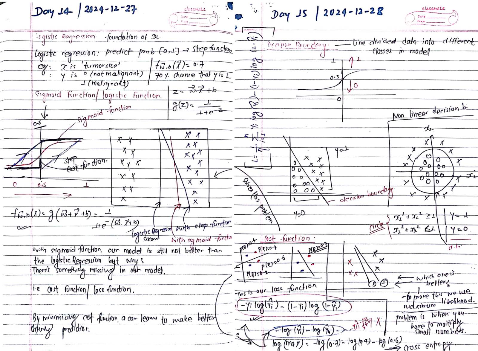
| Day14 | 2024-12-27 | Logistic Regression, Sigmoid Function | Machine Learning Specialization , CampusX |
| Day15 | 2024-12-28 | Decision Boundary, Cost Function | Machine Learning Specialization , CampusX |
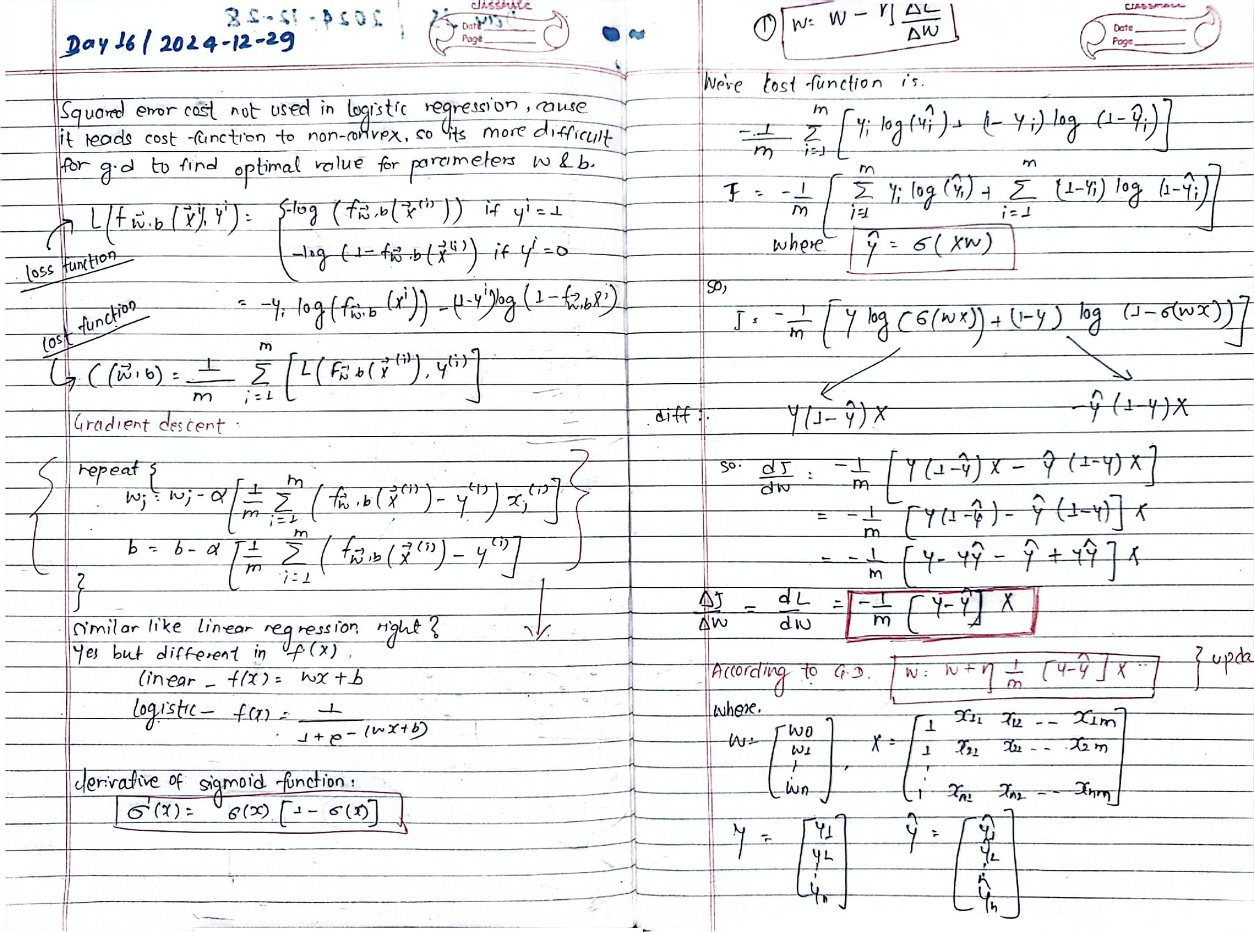
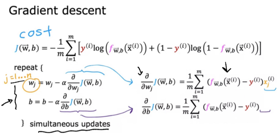
| Day16 | 2024-12-29 | Gradient Descent for logical regression | Machine Learning Specialization , CampusX |
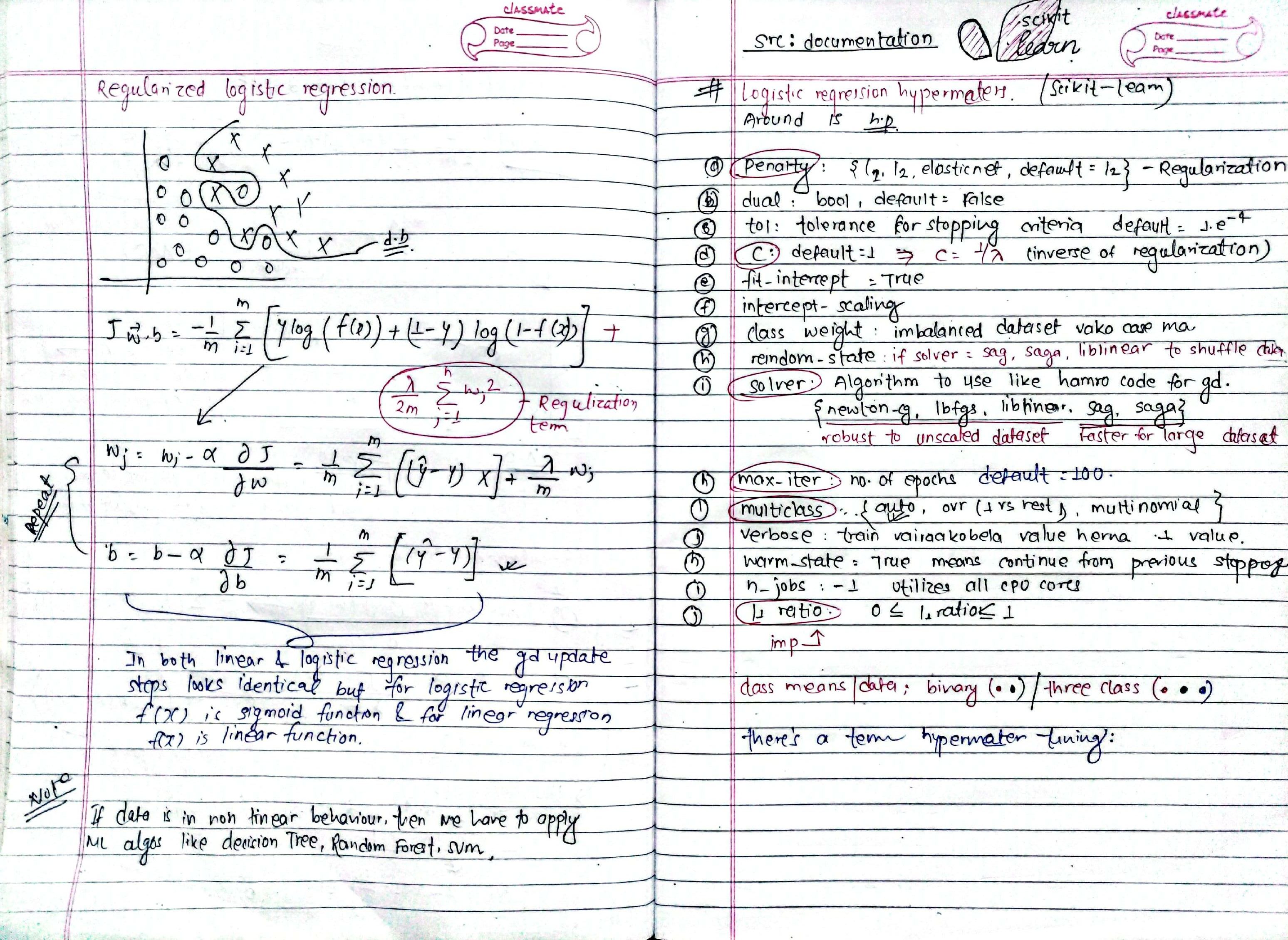
| Day17 | 2024-12-30 | Underfitting, Overfitting, Regularization Polynomial Features, Hyperparameters | Machine Learning Specialization |
| Day18 | 2024-12-31 | Neurons, Neural Netowrk, Forward Propagation | Machine Learning Specialization |
| Day19 | 2025-01-01 | Forward Propagation, Tensorflow implementations | Machine Learning Specialization |
| Day20 | 2025-01-02 | Building and comparing models (Binary Classification) | Machine Learning Specialization |
| Day21 | 2025-01-03 | Vectorization, Model training using Tensoflow | Machine Learning Specialization |
| Day22 | 2025-01-04 | Activation Functions, Softmax Intution | Machine Learning Specialization |
| Day23 | 2025-01-05 | Implementing Softmax | Machine Learning Specialization |
| Day24 | 2025-01-06 | Backpropagaton, What and how?? | Machine Learning Specialization |
| Day25 | 2025-01-07 | Backpropagation - Why? Advices for applying machine Learning | Machine Learning Specialization |
| Day26 | 2025-01-08 | Model selection, training test, cross validation, Bias and Variance, Learning curves | Machine Learning Specialization |
| Day27 | 2025-01-09 | Machine Learning Development Process, ML workflow | Machine Learning Specialization |
| Day28 | 2025-01-10 | Implementing ML model: Error Analysis and Transfer Learning | Notebook: Implementation, Machine Learning Specialization |
| Day29 | 2025-01-11 | Error Metrices, Encoding of Categorical Data, Transoformers | Machine Learning Specialization , CampusX |
| Day30 | 2025-01-12 | Scikit-Learn Pipelines & Ridge Regression (L2 Regularization) | Documentation: Scikit-Learn , CampusX |
| Day31 | 2025-01-13 | Lasso Regression (L1 Regularization), Elastic Net Regularization | ML playlist @CampusX |
| Day32 | 2025-01-14 | Decision Tree Emtropy and Information Gain | ML playlist @CampusX |
| Day33 | 2025-01-15 | Hyperparameters of Decision Tree with Scikit Learn, Regression Trees | ML playlist @CampusX , Visualize Yourself>> |
| Day34 | 2025-01-16 | Visualization Using DtreeViz(), Ensemble Learning | Github Repo: Dtreeviz, ML playlist @CampusX |
| Day35 | 2025-01-17 | Voting Ensemble >> Classification and Regression | ML playlist @CampusX , Visualize Yourself |
| Day36 | 2025-01-18 | Bagging Ensemble > Classification and Regression | ML playlist @CampusX |
| Day37 | 2025-01-19 | Random Forest: Intution, Working and difference with bagging, Random Forest Hyperparameters | ML playlist @CampusX |
| Day38 | 2025-01-20 | Boosting Ensemble: Adaboost Boosting | ML playlist @CampusX |
| Day39 | 2025-01-21 | Understanding GradientBoosting with Regression | ML playlist @CampusX |
| Day40 | 2025-01-22 | Gradient Boosting with Classification | ML playlist @CampusX , Vlog Link |
| Day41 | 2025-01-23 | XGboost Introduction | ML playlist @CampusX |
| Day42 | 2025-01-24 | XGBoost for Regression and Classification, Catboost Vs XGboost Vs LightGBM | ML playlist @CampusX ,Research Paper |
| Day43 | 2025-01-25 | Stacking Ensemble, Understanding Blending and K fold | ML playlist @CampusX |
| Day44 | 2025-01-26 | K-Nearest Neighbor, Coding KNN from Scratch | ML playlist @CampusX |
| Day45 | 2025-01-27 | Support Vector Machine | ML playlist @CampusX |
| Day46 | 2025-01-28 | K-Means Clustering, DBSCAN | Notebook: K-Means clustering Demo , Notebook: DBSCAN demo |
| Day47 | 2025-01-29 | Hierarchical Clustering, Silhouette Score | Kaggle, ML playlist @CampusX |
| Day49 | 2025-01-30 | PCA (Principle Component Analysis), Implementing with MNIST dataset | Notebook: Applying PCA on MNIST dataset |
| Day50 | 2025-02-01 | Visualizing and Comparing PCA, t-SNE, UMAP, and LDA + Revision with the course ML specialization | Machine Learning Specialization |
| Day51 | 2025-02-02 | Anomaly Detection | Machine Learning Specialization, Notebook: Anomaly Detection |
| Day52 | 2025-02-03 | Collaborative Filtering | Machine Learning Specialization |
| Day53 | 2025-02-04 | Project @ Football Players Market Value Prediction - Introduction and Planning | Project Plan |
| Day54 | 2025-02-05 | Project @ Football Players Market Value Prediction - Collecting Data (Scraping) | Notebook |
| Day55 | 2025-02-06 | Project @ Football Players Market Value Prediction - Cleaning Data | Notebook |
| Day56 | 2025-02-07 | Project @ Football Players Market Value Prediction - EDA | Notebook |
| Day57 | 2025-02-08 | Project @ Football Players Market Value Prediction - Feature Engineering: (Creating features, Transforming Features) | Notebook |
| Day58 | 2025-02-09 | Project @ Football Players Market Value Prediction - ML: (Linear Regression with Refined Features and deploying with Streamlit) | Notebook |
| Day59 | 2025-02-10 | Project @ Complete Streamlit setup for Linear Regression | Streamlit Documentation |
| Day60 | 2025-02-11 | Project @ Testing Ridge, Lasso, and Decision Trees | Project @ Football Players Market Value Prediction |
| Day61 | 2025-02-12 | Project @ Had to hit reset from Feature Engineering | Project @ Football Players Market Value Prediction |
| Day62 | 2025-02-13 | Project @ Finalizing Project and Deploying it | Project @ Football Players Market Value Prediction |
| Day63 | 2025-02-14 | Content-Based Movie Recommender System - Preprocessing | Notebook |
| Day64 | 2025-02-15 | Content-Based Movie Recommender System - Building and Deployment | Live Demo |
| Day65 | 2025-02-16 | Diving into Deep Learning | Intro to Deep Learning @MIT |
| Day66 | 2025-02-17 | Perceptrons | Deep learning playlist @ CampusX |
| Day67 | 2025-02-18 | Perceptron, Loss function and gradient Descent | Deep learning playlist @ CampusX , Grokking Deep Learning @Andrew W. Trask |
| Day68 | 2025-02-19 | Multilayer Perceptron | Deep learning playlist @ CampusX |
| Day69 | 2025-02-20 | MLP notation, Forward Propagation | Deep learning playlist @ CampusX |
| Day70 | 2025-02-21 | Loss Functions for deep learning | Deep learning playlist @ CampusX |
| Day71 | 2025-02-22 | Backpropagation, deep diving this time | Deep learning playlist @ CampusX |
| Day72 | 2025-02-23 | Implementing Backpropagation for Regression | Notebook: Backpropagation Regression |
| Day73 | 2025-02-24 | Implementing Backpropagation for Classification | Notebook: Implementation Backprop Classification |
| Day74 | 2025-02-25 | Revising old days, Memoization | Deep learning playlist @ CampusX |
| Day75 | 2025-02-26 | Vanishing Gradient, Exploding Gradient | Deep learning playlist @ CampusX |
| Day76 | 2025-02-27 | Implementing artificial neural networks (ann) for different datasets | Deep learning playlist @ CampusX |
| Day77 | 2025-02-28 | Improving Neural Networks | Deep learning playlist @ CampusX |
| Day78 | 2025-03-01 | Sequence Modeling / RNNs - Just Overview | Intro to Deep Learning @MIT |
| Day79 | 2025-03-02 | Transformers Attention - Just Overview | Intro to Deep Learning @MIT |
| Day80 | 2025-03-03 | CNNs - Just Overview Part 1 | Intro to Deep Learning @MIT |
| Day81 | 2025-03-04 | CNNs - Just Overview Part 2 | Intro to Deep Learning @MIT |
| Day82 | 2025-03-05 | Deep Generative Modeling - Just Overview | Intro to Deep Learning @MIT |
| Day83 | 2025-03-06 | Reinforcement Learning - Just Overview | Intro to Deep Learning @MIT |
| Day84 | 2025-03-07 | Deep Learning: Challenges & New Frontiers - Just Overview | Intro to Deep Learning @MIT |
| Day85 | 2025-03-08 | Early Stopping & Normalizing Inputs, Droput | Deep learning playlist @ CampusX, Grokking Deep Learning @Andrew W. Trask |
| Day86 | 2025-03-09 | Regularization, Quantization | Deep learning playlist @ CampusX |
| Day87 | 2025-03-10 | Activation Functions - Revisited | Deep learning playlist @ CampusX |
| Day88 | 2025-03-11 | Weight Initialization | Deep learning playlist @ CampusX |
| Day89 | 2025-03-12 | Deep Learning Optimizers | Deep learning playlist @ CampusX |
| Day90 | 2025-03-13 | Keras Tuner | Deep learning playlist @ CampusX |
| Day91 | 2025-03-14 | Deep Diving into CNNs | Deep learning playlist @ CampusX |
| Day92 | 2025-03-15 | Understanding Paddings and Strides | Deep learning playlist @ CampusX |
| Day93 | 2025-03-16 | Backpropagation in CNNs: A Quick Breakdown | Deep learning playlist @ CampusX, Grokking Deep Learning @Andrew W. Trask |
| Day94 | 2025-03-17 | LeNet5, Cat Vs Dog Classification | Deep learning playlist @ CampusX, Grokking Deep Learning @Andrew W. Trask |
| Day95 | 2025-03-18 | GPU slow than CPU - well in my case? | Deep learning playlist @ CampusX |
| Day96 | 2025-03-19 | Data Augmentation, Pretrained Models | Deep learning playlist @ CampusX, Grokking Deep Learning @Andrew W. Trask |
| Day97 | 2025-03-20 | Visualizing Convolutional Layers, Transfer Learning | Deep learning playlist @ CampusX, Grokking Deep Learning @Andrew W. Trask |
| Day98 | 2025-03-21 | Keras Functional API | Deep learning playlist @ CampusX , Article |
| Day99 | 2025-03-21 | Finalizing Dog Cat Classifier Project | Project - Live Demo |
| Day100 | 2025-03-23 | Hidden Markov Model, Quantum Machine Learning | Medium Article: Understanding Hidden Markov Models |
| Day101 | 2025-03-24 | Exploring Pytorch Surfacely | DL with Pytorch - Datacamp |
| Day102 | 2025-03-25 | Training a neural network with pytorch | DL with Pytorch - Datacamp |
| Day103 | 2025-03-26 | Evaluating and improving models | DL with Pytorch - Datacamp |
| Day104 | 2025-03-27 | Crawling through DL with pytroch | Deep Learning for Coders -Fast.Ai, @CampusX |
| Day105 | 2025-03-28 | Starting chapter 2 : from model to production | Deep Learning for Coders -Fast.Ai, @CampusX |
| Day106 | 2025-03-29 | Exploring Autograd and Portfolio Tweaks | Deep Learning for Coders -Fast.Ai, @CampusX |
| Day107 | 2025-03-30 | Refining Portfolio whole day | Deep Learning for Coders -Fast.Ai, @CampusX |
| Day108 | 2025-03-31 | Autograd in PyTorch: Deeper Understanding | Deep Learning for Coders -Fast.Ai, @CampusX |
| Day109 | 2025-04-01 | PyTorch Training Pipeline (Manual + Using nn.Module) | Deep Learning for Coders -Fast.Ai, @CampusX |
| Day110 | 2025-04-02 | Dataset & DataLoader Class in PyTorch | Deep Learning for Coders -Fast.Ai, @CampusX |
| Day111 | 2025-04-03 | ANN on Fashion MNIST, GELU | Deep Learning for Coders -Fast.Ai, @CampusX |
| Day112 | 2025-04-04 | ANN on larger FMNIST dataset with GPU (local), GELU/SiLU history | Deep Learning for Coders -Fast.Ai, @CampusX |
| Day113 | 2025-04-05 | Optimizing FMNIST NN using Dropouts, Regularization and Batch Normalization in Pytorch | Notebook |
| Day114 | 2025-04-08 | RNNs revisited, Karpathy's blog, Project Planning | Karpathy Blog |
| Day115 | 2025-07-08 | Classifying Footballers with their Eyes - Day 1 | Project Notebook |
| Day116 | 2025-07-09 | Classifying Footballers with their Eyes – Day 2 | Project Notebook |
| Day117 | 2025-07-10 | YOLO (You Only Look Once) | YOLO Paper |
| Day118 | 2025-07-11 | LSTM, GRU & Encoder-Decoder Architecture | Colah's Blog |
| Day119 | 2025-07-12 | Bahdanau Attention and Luong Attention | Bahdanau Paper |
| Day120 | 2025-07-13 | Building a Seq2Seq Chatbot – Data Preparation & Preprocessing | PyTorch Tutorial |
| Day121 | 2025-07-14 | Building a Seq2Seq Chatbot - Defining Model (encoder, attention, decoder) | Notebook |
| Day122 | 2025-07-15 | Building a Seq2Seq Chatbot – Evaluation / Deployment | Live Demo |
| Day123 | 2025-07-20 | Transformers – Deep Dive into Attention and Architecture | Attention Paper |
| Day124 | 2025-07-21 | Transformers – Vitals [understanding everything] | Transformer Guide |
| Day125 | 2025-07-22 | GPT from Scratch - Project Setup | Karpathy's Tutorial |
| Day126 | 2025-07-23 | GPT from Scratch - Bigram Language Model | Notebook |
| Day127 | 2025-07-24 | GPT from Scratch - Self-Attention | Notebook |
| Day128 | 2025-07-25 | GPT from Scratch – Complete Transformer | Notebook |
| Day129 | 2025-07-26 | Image Captioning – Kickoff | Notebook |
| Day130 | 2025-07-27 | Image Captioning – Feature Extraction & Pipeline | Notebook |
| Day131 | 2025‑07‑28 | Image Captioning – Training & Deployment | Build a Large Language Model from Scratch |
| Day132 | 2025‑07‑29 | Tokenizer Tricks (Subword, Byte-Pair Encoding) + Comparing Architectures | Build a Large Language Model from Scratch |
| Day133 | 2025‑07‑30 | Implementing seq2seq (Diff Approach of Visualizations) | Build a Large Language Model from Scratch |
| Day134 | 2025‑07‑31 | Implementing Transformer Encoder/Decoder Again | Build a Large Language Model from Scratch |
| Day135 | 2025‑08‑01 | Pretraining on Unlabeled Data, Evaluating, Loading Pretrained Weights | Build a Large Language Model from Scratch |
| Day136 | 2025‑08‑02 | Finetuning – Classification | Build a Large Language Model from Scratch |
| Day137 | 2025‑08‑03 | Finetuning – Teaching LLMs to Follow Prompts and Perform Complex Tasks, Visualizations | Build a Large Language Model from Scratch |
| Day137 | 2025‑08‑03 | Finetuning – Teaching LLMs to Follow Prompts and Perform Complex Tasks, Visualizations | Build a Large Language Model from Scratch |
| Day138 | 2025‑08‑04 | LLM Fine-Tuning & Evaluation | Build a Large Language Model from Scratch |
| Day139 | 2025‑08‑05 | Exploring Hugging Face Transformers | Build a Large Language Model from Scratch |
| Day140 | 2025‑08‑06 | Project – Sentiment Analysis [Planning] + Exploring ViT | Notebook, Kaggle Code |
| Day141 | 2025‑08‑07 | Project – Sentiment Analysis [Preprocessing] + ViT Architecture | Kaggle Code |
| Day142 | 2025‑08‑08 | Project – Sentiment Analysis [EDA + Testing GloVe] | Notebook, Notebook, Kaggle Code |
| Day143 | 2025‑08‑09 | Project – Sentiment Analysis [Advanced Architectures] | Notebook, Notebook, Kaggle Code |
| Day144 | 2025‑08‑10 | Project – Sentiment Analysis [App Deployment] | Live Demo, Code |
| Day145 | 2025‑08‑11 | Diving Deep into Vision Transformers (ViTs) | Blog |
| Day146 | 2025‑08‑12 | Diving into Diffusion Models | Video |
| Day147 | 2025‑08‑13 | Diffusion Model Deep Dive | Paper |
| Day148 | 2025‑08‑15 | Naive Bayes & Gaussian Mixture Models | Langchain Playlist |
| Day149 | 2025‑08‑17 | Introduction to Langchain | Langchain Playlist |
| Day150 | 2025‑08‑18 | Introduction to Langchain Components | Langchain Playlist |
| Day151 | 2025‑08‑19 | Deep Dive into Langchain Models | Langchain Playlist |
| Day152 | 2025‑08‑20 | Langchain Prompts and Building a Simple Chatbot | Langchain Playlist |
| Day153 | 2025‑08‑21 | Structured Output with Langchain | Langchain Playlist |
| Day154 | 2025‑08‑23 | Langchain Output Parsers | Langchain Playlist |
| Day155 | 2025‑08‑24 | Langchain Chain Fundamentals (Simple, Sequential, Parallel, Conditional Chains) | Langchain Playlist |
| Day156 | 2025‑08‑25 | Langchain Runnables (Modular Components, Composable Workflows) | Langchain Playlist |
| Day157 | 2025‑08‑26 | Runnable Modules Deep Dive (Sequence, Parallel, Passthrough, Lambda, Branch) | Langchain Playlist |
| Day158 | 2025‑08‑27 | Document Loaders & Text Splitters (RAG Foundations) | Langchain Playlist |
| Day159 | 2025‑08‑28 | Vector Stores in Langchain (Chroma, CRUD Operations, Similarity Search) | Langchain Playlist |
| Day160 | 2025‑08‑29 | Retrievers & Few-Shot Learning (Wikipedia, Vector, MMR, MultiQuery, Contextual) | Langchain Playlist |
| Day161 | 2025‑08‑30 | RAG Application for UCL Draw (Text Splitting, Vector Embeddings, Response Generation) | Langchain Playlist |
| Day162 | 2025‑08‑31 | Langchain Tools (Built-in & Custom, Tool Calling & Binding) | Langchain Playlist |
| Day163 | 2025‑09‑01 | Langchain Agents (Zero-Shot, Conversational, ReAct DocStore, Self-Ask) | Langchain Playlist |
| Day164 | 2025‑09‑02 | Local Agent with Ollama & Langchain (ChromaDB, RAG) | Langchain Playlist |
| Day165 | 2025‑09‑03 | Introduction to LangGraph (Stateful Agent Workflows) | Langgraph Playlist |
| Day166 | 2025‑09‑04 | Agentic AI Fundamentals (Autonomy, Components, Planning, Memory) | Langchain Playlist |
| Day167 | 2025‑09‑05 | LangChain vs LangGraph Comparison (State Management, Chatbot Example) | Langgraph Playlist |
| Day168 | 2025-09-06 | Building a Branching Chatbot | Langgraph Playlist |
| Day169 | 2025-09-07 | Persistence with Checkpoints | Langgraph Playlist |
| Day170 | 2025-09-08 | Exploring LangSmith | Langgraph Playlist |
| Day171 | 2025-09-11 | Contextual Q&A with Memory | Langchain Playlist |
| Day172 | 2025-09-12 | Bhagavad Gita Expert Chatbot | Langgraph Playlist |
| Day173 | 2025-09-13 | Multi-Agent Debating System | Langgraph Playlist |
| Day174 | 2025-09-14 | Debate Agent App Completion | Langgraph Playlist |
| Day175 | 2025-09-15 | Introduction to FastAPI for ML | FastAPI Documentation |
| Day176 | 2025-09-16 | FastAPI Implementation | FastAPI Documentation |
| Day177 | 2025-09-17 | HTTP Request Methods and REST Architecture | FastAPI Documentation |
| Day178 | 2025-09-18 | FastAPI Parameters and Request Body | FastAPI Documentation |
| Day179 | 2025-09-19 | Mini Project with FastAPI | FastAPI Documentation |
| Day180 | 2025-09-20 | Building Industry-Ready APIs with FastAPI | FastAPI Documentation |
| Day181 | 2025-09-23 | Containerizing FastAPI Applications | FastAPI Documentation |
| Day182 | 2025-09-24 | fastapi deployment on aws | aws docs |
| Day183 | 2025-09-25 | project setup – choose your own adventure | project repo |
| Day184 | 2025-09-26 | database design and core components | project repo |
| Day185 | 2025-09-27 | api implementation and background tasks | project repo |
| Day186 | 2025-09-28 | backend completion and debugging | project repo |
| Day187 | 2025-09-29 | frontend integration and project completion | project repo |
| Day188 | 2025-10-01 | concurrency patterns in fastapi | starlette concurrency |
| Day189 | 2025‑10‑02 | self-supervised learning – foundations | Lil'Log SSL Blog |
| Day190 | 2025‑10‑03 | mcp and lazy week | Masked Conditional Prediction |
| Day191 | 2025‑10‑04 | ssrl – image & video approaches | Lil'Log SSRL |
| Day192 | 2025‑10‑05 | wrapping up ssl + fun reads | Postgres vs SQLite, GPT Speculations |
| Day193 | 2025‑10‑06 | llama2 fine-tuning with qlora | QLoRA Fine-Tuning Guide |
| Day194 | 2025‑10‑12 | gemma 2 fine-tuning using unsloth | Gemma2 Fine-tuning Notebook |
| Day195 | 2025‑10‑13 | saving & loading lora adapters, explored "lora without regret" | LoRA Blog Post |
| Day196 | 2025‑10‑14 | attempted RAG evaluation, faced compatibility issues | MCP Documentation |
| Day197 | 2025‑10‑16 | built a custom MCP server, integrated with Cursor | Custom Implementation |
| Day198 | 2025‑10‑18 | studied RL fundamentals: policies, MDPs, rewards | HuggingFace RL Course |
| Day199 | 2025‑10‑20 | explored Q-learning & Deep Q-learning, lunar lander env | HuggingFace RL Course |
| Day200 | 2025‑10‑21 | trained PPO agent on LunarLander-v3 using SB3 | HuggingFace RL Course |
Day 01: Basics of Linear Algebra
linear algebra is used to represent data, perform matrix operations, and solve equations in algorithms like regression, pca, and neural networks.
-
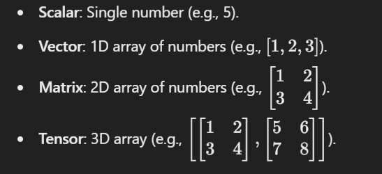
Scalars, Vectors, Matrices, Tensors: Basic data structures for ML.
-
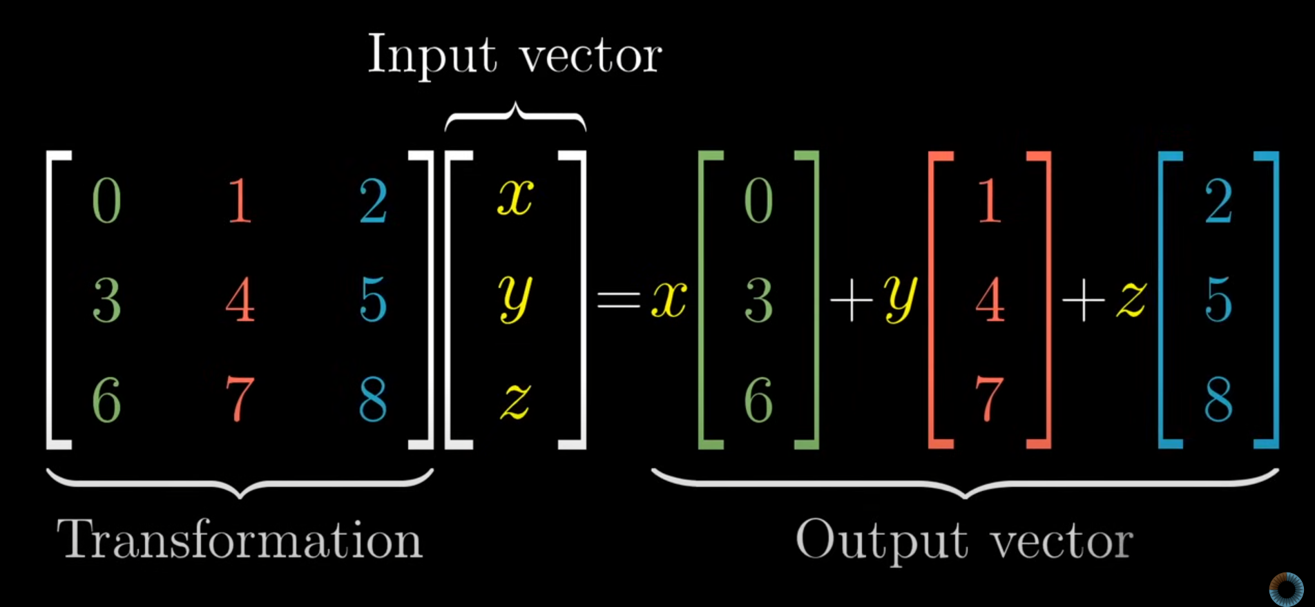
Linear Combination and Span: Representing data points as weighted sums. Used in Linear Regression and neural networks.
-
Determinants: Matrix invertibility, unique solutions in linear regression.
-
Dot and Cross Product: Similarity (e.g., in SVMs) and vector transformations.

Slow progress right?? but consistent wins the race!
Day 02: Decomposition, Derivation, Integration, and Gradient Descent
-
Identity and Inverse Matrices: Solving equations (e.g., linear regression) and optimization (e.g., gradient descent).
-
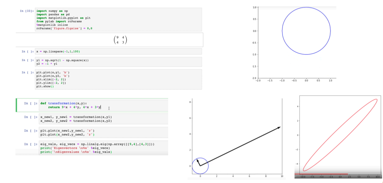
Eigenvalues and Eigenvectors: PCA, SVD, feature extraction; eigenvalues capture variance.
-
Singular Value Decomposition (SVD): PCA, image compression, and collaborative filtering.
Calculus Overview:
-
Functions & Graphs: Relationship between input (e.g., house size) and output (e.g., house price).
-
Derivatives: Adjust model parameters to minimize error in predictions (e.g., house price).
-
Partial Derivatives: Measure change with respect to one variable, used in neural networks for weight updates.
-
Gradient Descent: Optimization to minimize the cost function (error).
-
Optimization: Finding the best values (minima/maxima) of a function to improve predictions.
-
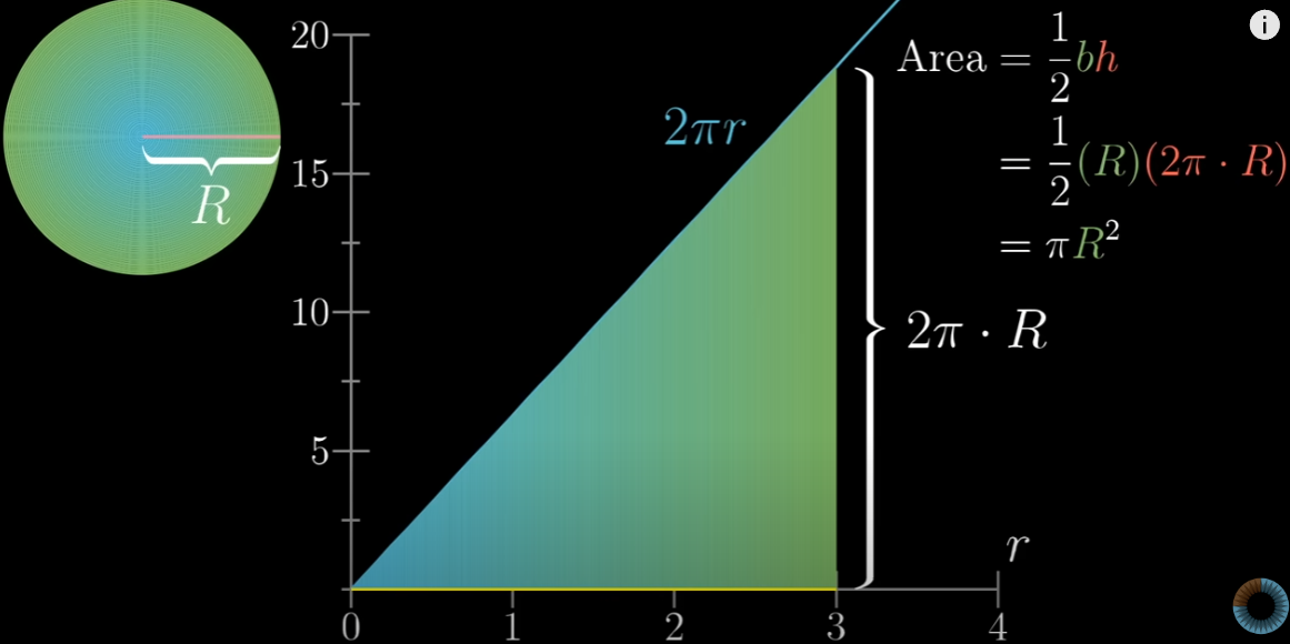
Integrals: Calculate area under a curve, used in probabilistic models (e.g., Naive Bayes).
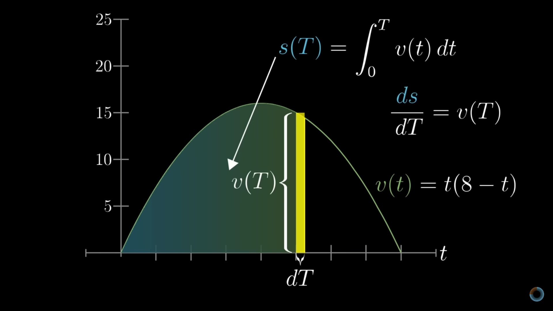
Revised statistics and probability concepts. Ready for the ML Specialization course!
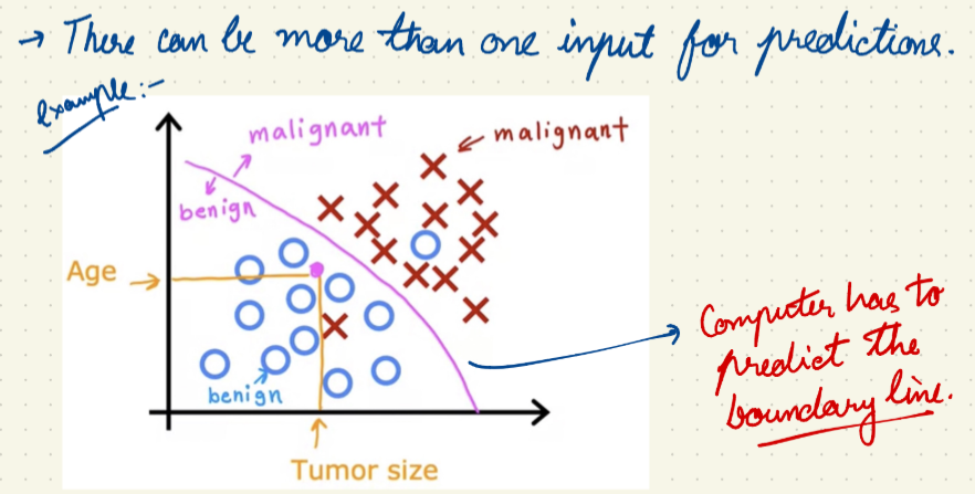
Day 03: Supervised Machine Learning: Regression and Classificaiton
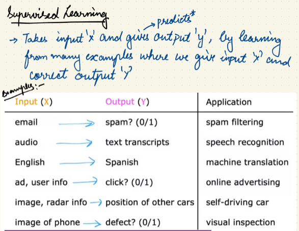
- Supervised Learning:

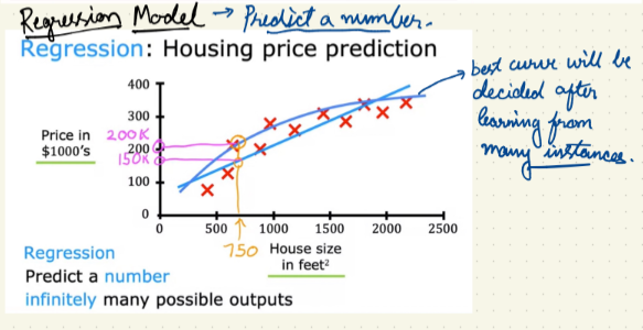
- Regression:
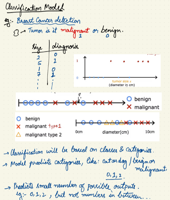
- Classification:
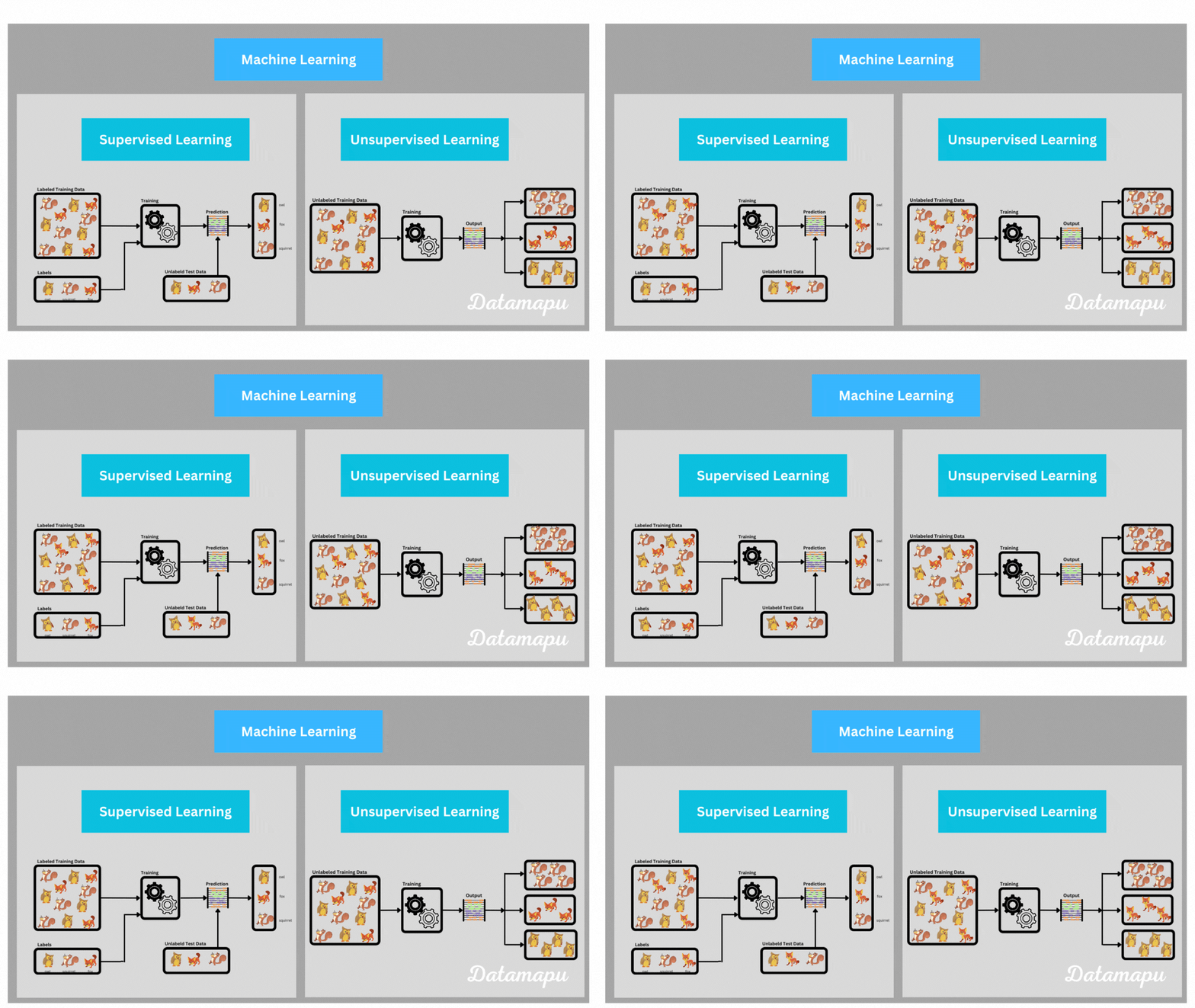
Day 04: Unsupervised Learning: Clustering, dimensionality reduction
data only comes with input x, but not output labels y. Algorithm has to find structure in data.
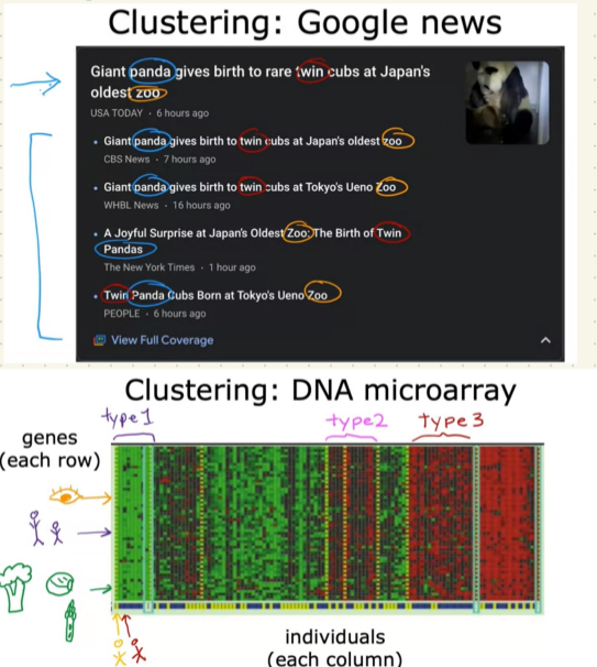
- Clustering: group similar data points together
- dimensionality reduction: compress data using fewer numbers eg image compression
- anomaly detection: find unusual data points eg fraud detection
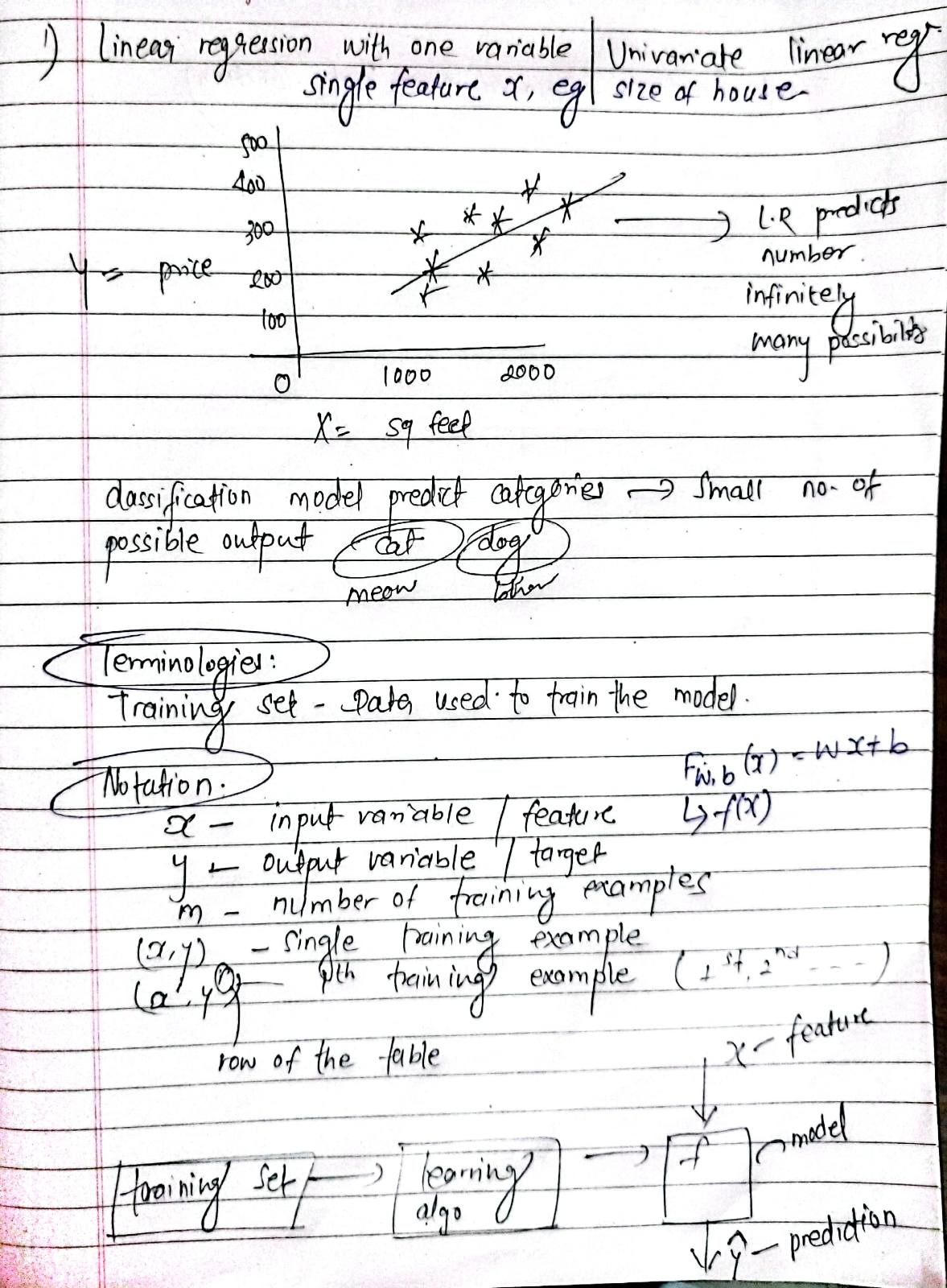
Day 05: Univariate Linear Regression:
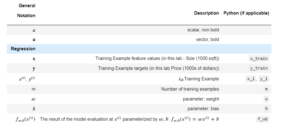
- Learned univariate linear regression and practiced building a model to predict house prices using size as input, including defining the hypothesis function, making predictions, and visualizing results.
Notebook: Model Representation
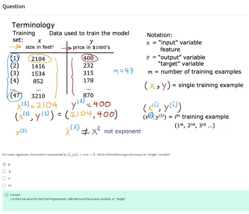
 - Univariate Linear Regression Quiz
Day 06: Cost Function:
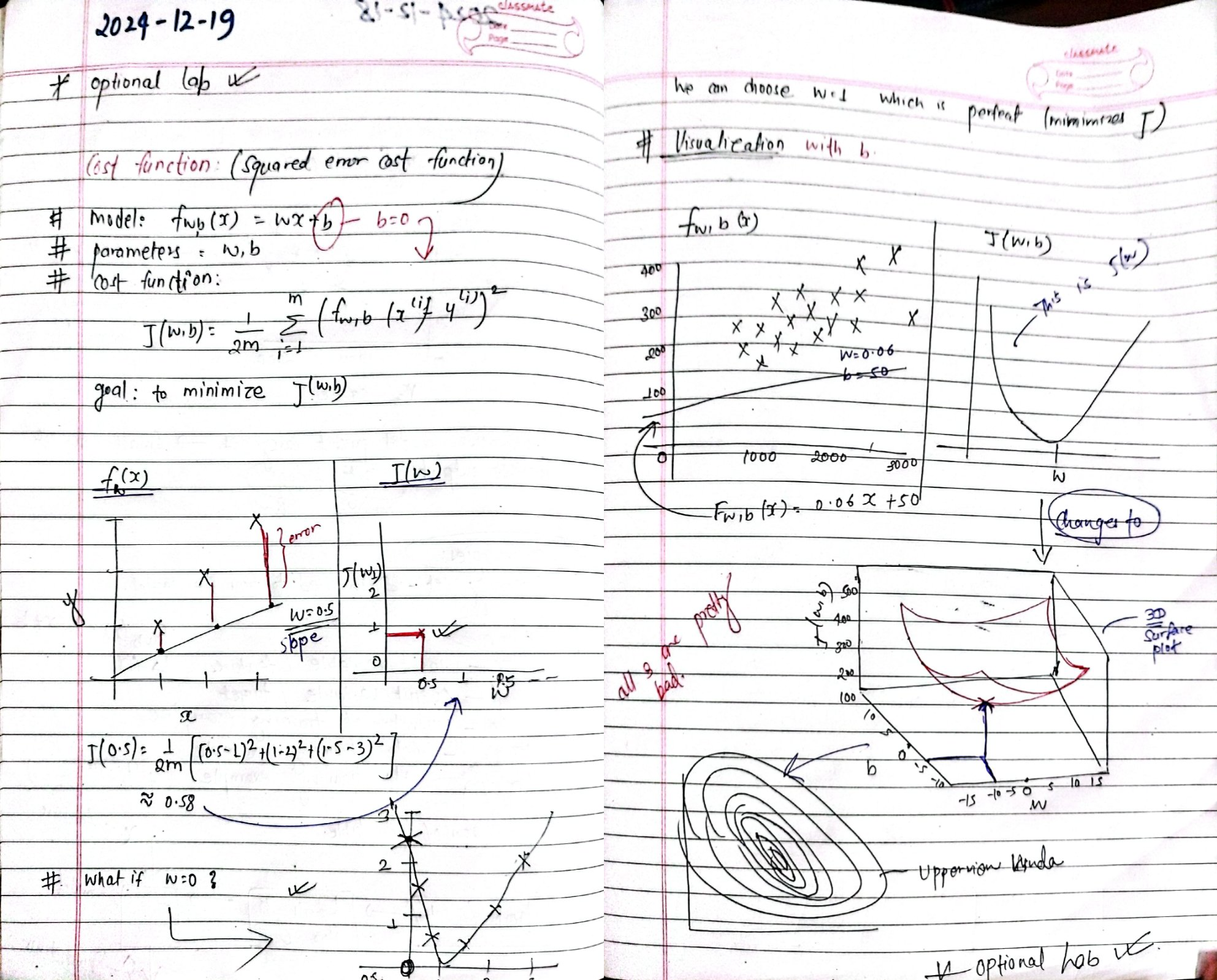 Visualization of cost function:
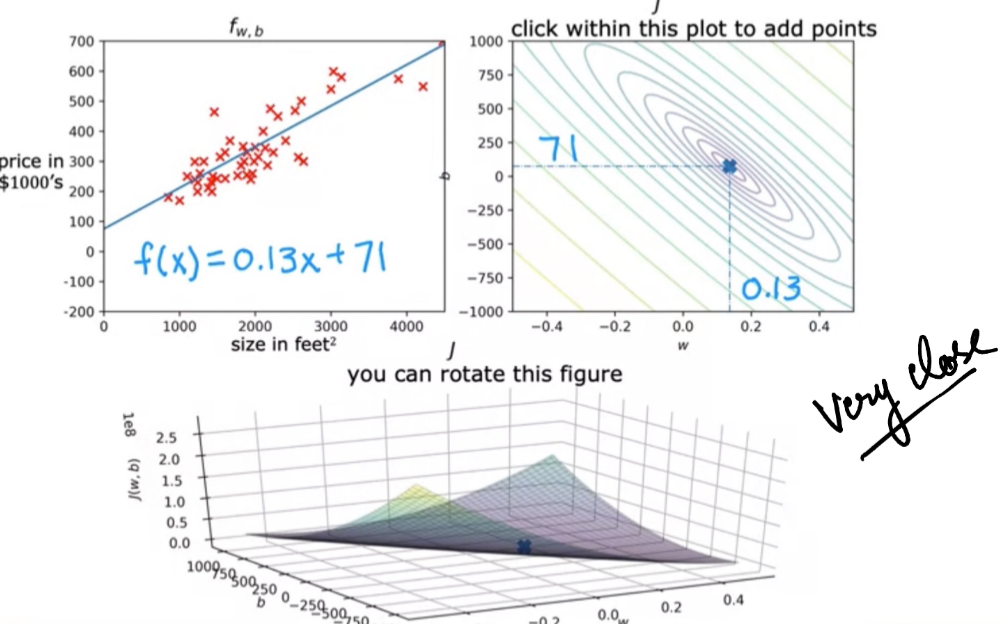
- manually reading these contour plot is not effective or correct, as the complexity increases, we need an algorithm which figures out the values w, b (parameters) to get the best fit time, minimizing cost function
Notebook: Model Representation
Gradient descent is an algorithm which does this task
Day 07: Gradient Descent
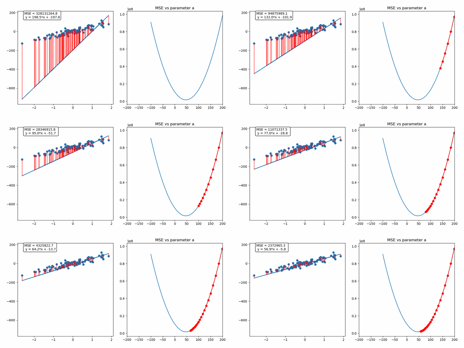 learned the basics by assuming slope constant and with only the vertical shift.
later learned GD with both the parameters w and b.
learned the basics by assuming slope constant and with only the vertical shift.
later learned GD with both the parameters w and b.
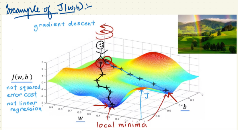
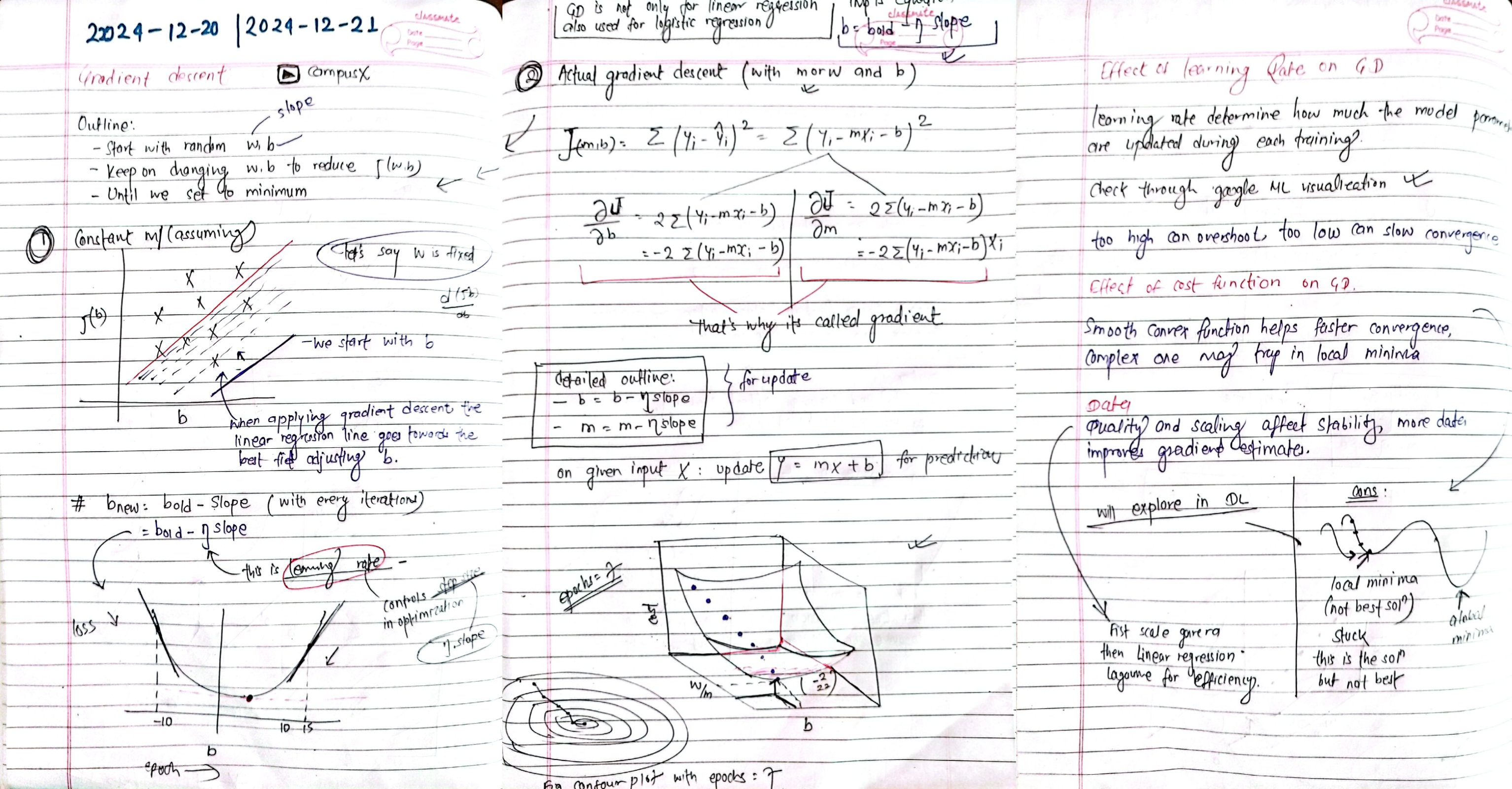
Day 08: Effect of learning Rate, Cost function and Data on GD
- learning rate on GD:Affects the step size; too high can overshoot, too low can slow convergence
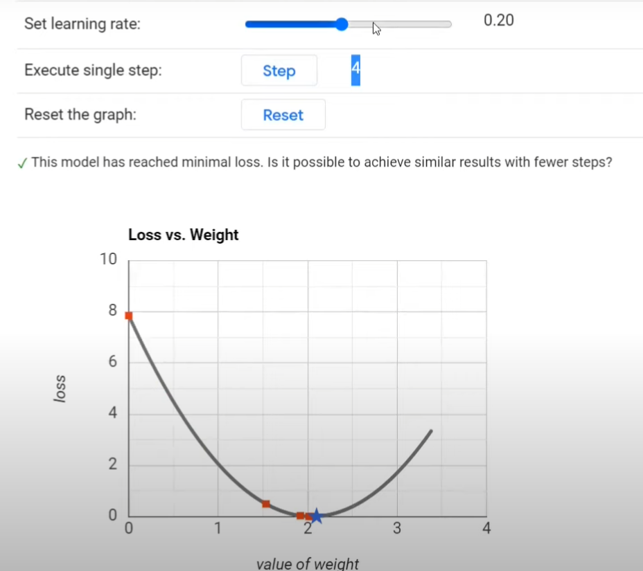
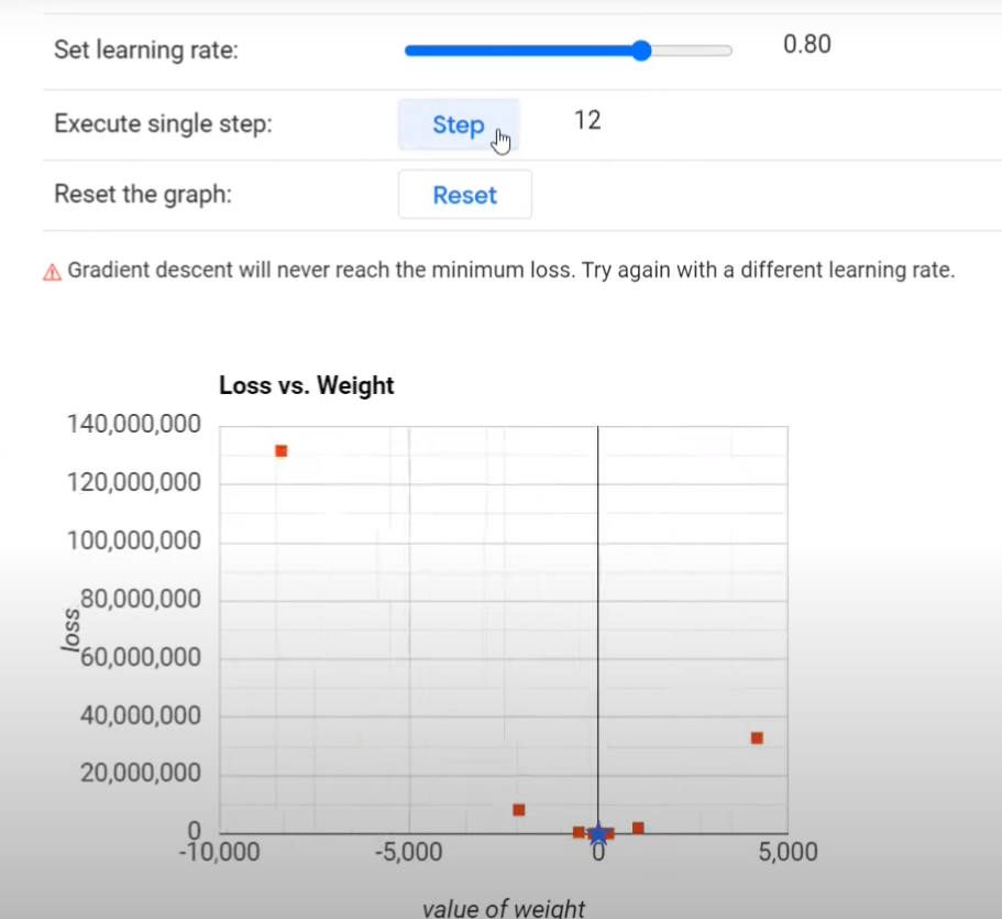 - cost function on GD:Smooth, convex functions help faster convergence; complex ones may trap in local minima
- Data on GD:Quality and scaling affect stability; more data improves gradient estimates
Notebook: gradient descent animation 3d
Day 09: Linear Regression with multiple features, Vectorization
Predicts target using multiple features, minimizing error.
- Vectorization: Matrix operations replace loops for faster calculations.

Day10: Feature Scaling
Today, I learned about feature scaling and how it helps improve predictions. There are multiple methods for feature scaling, including
- Min-Max Scaling
- Mean Normalization
- Z-Score Normalization
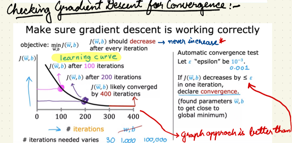
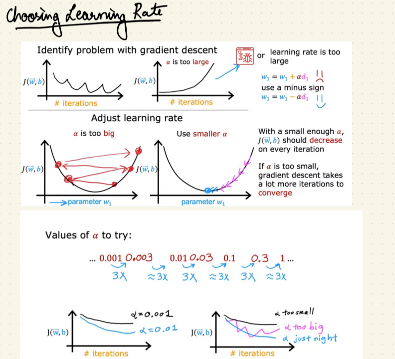
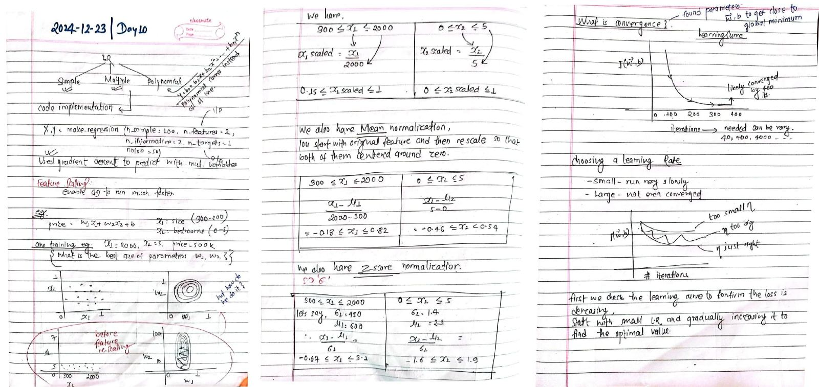 To ensure proper convergence:
check the learning curve to confirm the loss is decreasing.
Start with a small learning rate and gradually increase to find the optimal value.
To ensure proper convergence:
check the learning curve to confirm the loss is decreasing.
Start with a small learning rate and gradually increase to find the optimal value.
Day 11: Feature engineering and Polynomial Regression
feature engineering improves features to better predict the target.
eg If we need to predict the cost of flooring and have length and breadth of the room as features, we can use feature engineering to create a new feature, area (length × breadth), which directly impacts the flooring cost.
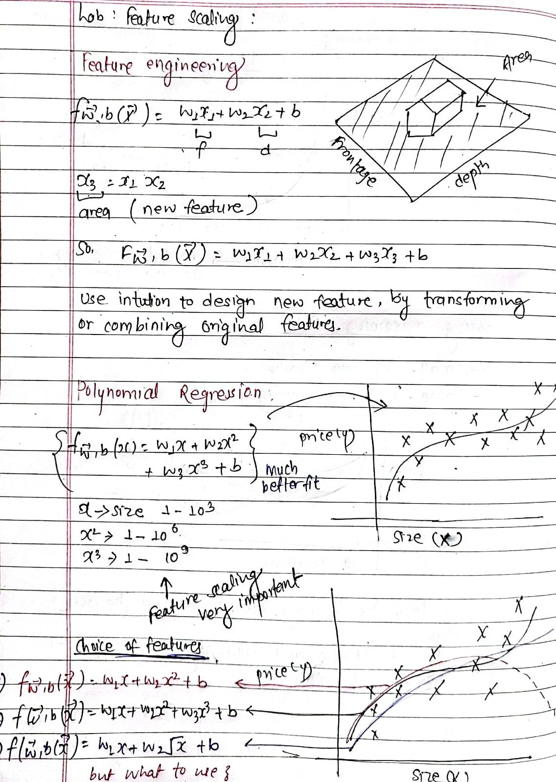 

explored polynomial regression that models the relationship between variables as a polynomial curve instead of a straight line
Equation:
y = b₀ + b₁x + b₂x² + ... + bₙxⁿ
It is useful for capturing nonlinear relationships in data.
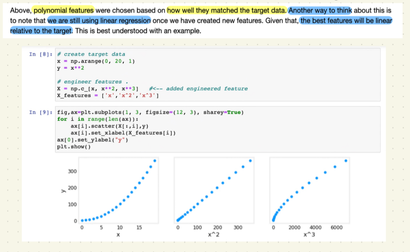
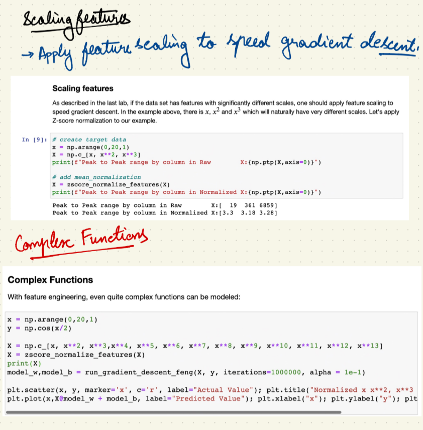
Lab1: Feature Scaling and Learning Rate
Lab2: Feature Engineering and PolyRegression
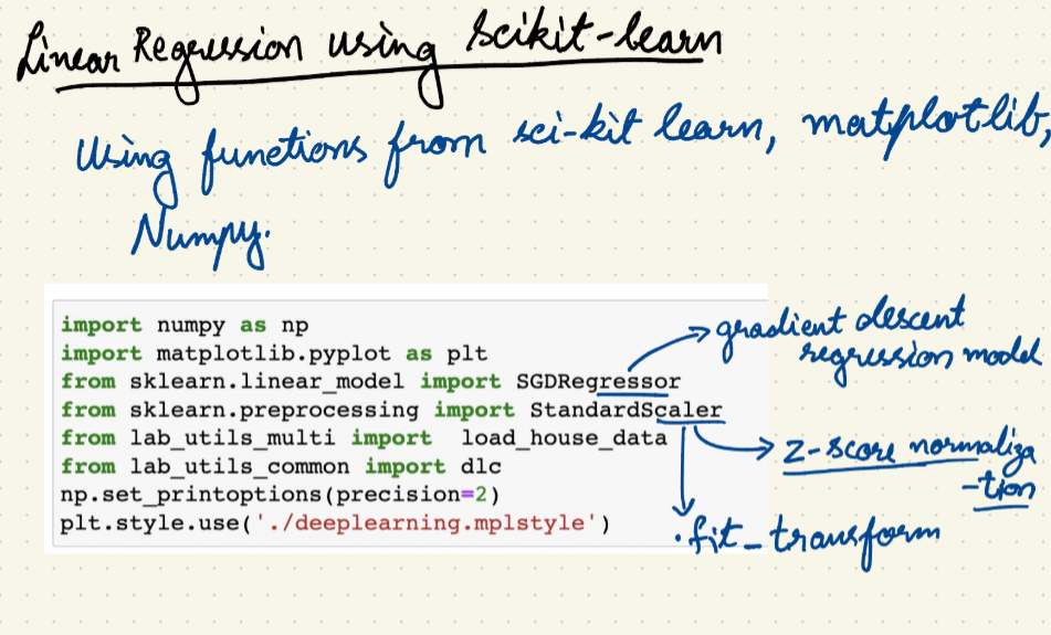
Day 12: Linear Regression using Scikit Learn
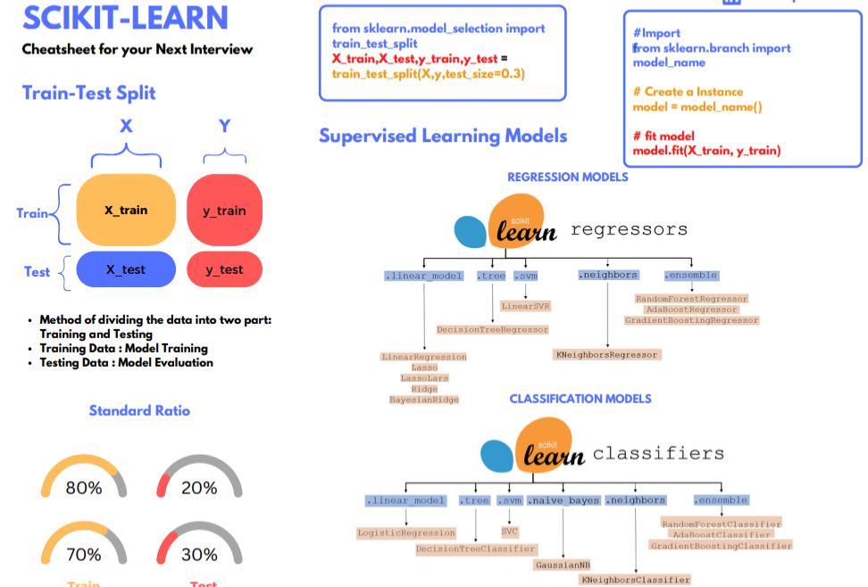
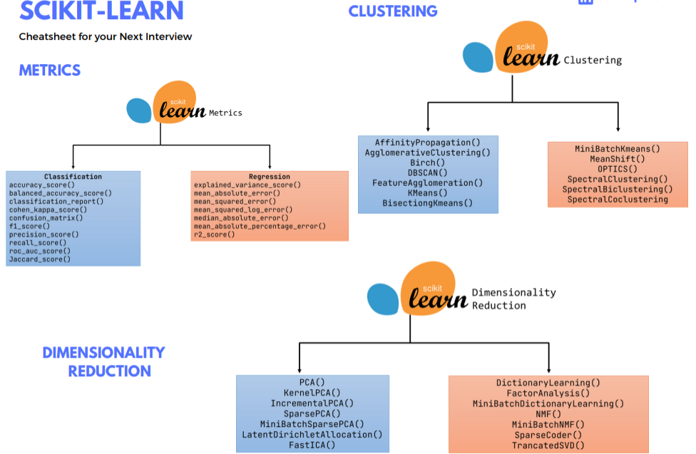
Had a productive session with linear regression in scikit learn. The lab helped me get a better grasp of the process, though I need more practice with tuning models. Also revisited the Scikit-Learn models ,more comfortable with them now
- Scikit-learn is an open-source Python library used for machine learning that provides simple and efficient tools for data analysis, including algorithms for classification, regression, clustering, and dimensionality reduction.

Day 13: Classification
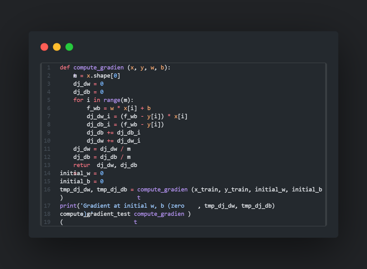
Notebook: Graded Lab
Notebook: Classification solution
- Classification is the process of categorizing items into different groups based on shared characteristics, like classifying tumors into benign (non-cancerous) and malignant (cancerous) based on their growth behavior and potential to spread.
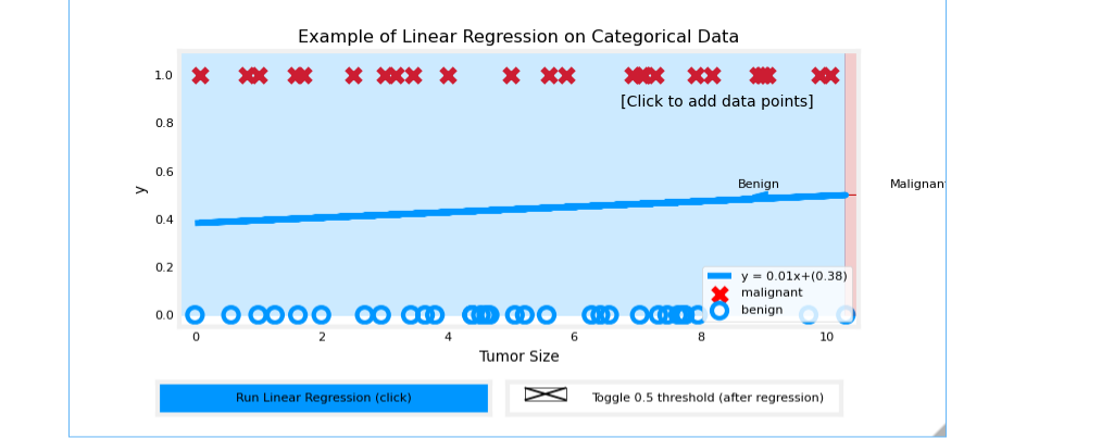 The example above demonstrates that the linear model is insufficient to model categorical data. The model can be extended as described in the following lab.
Day 14: Logistic Regression, Sigmoid Function
- Logistic Regression: A classification algorithm used to predict probabilities of binary outcomes.
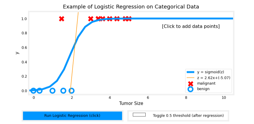
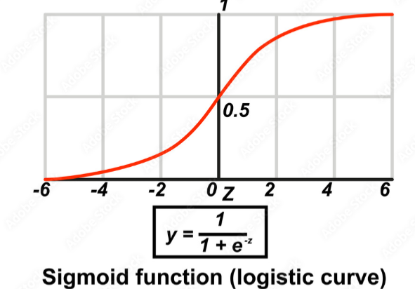
- Sigmoid Function: A mathematical function that maps any input to a value between 0 and 1, used in logistic regression to model probabilities.
Day 15: Decision Boundary, Cost Function
- Decision Boundary: A line or surface that separates different classes in a classification problem based on the model’s predictions.
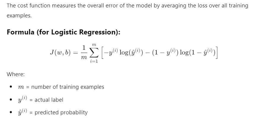
- cost function:
Day 16: Gradient Descent for Logical Regression
Notebook: Gradient Descent Model implementation
Notebook: GD with Scikit-learn
Learned logistic regression cost, gradient descent, and sigmoid derivatives through step-by-step derivations and comparisons with linear regression.
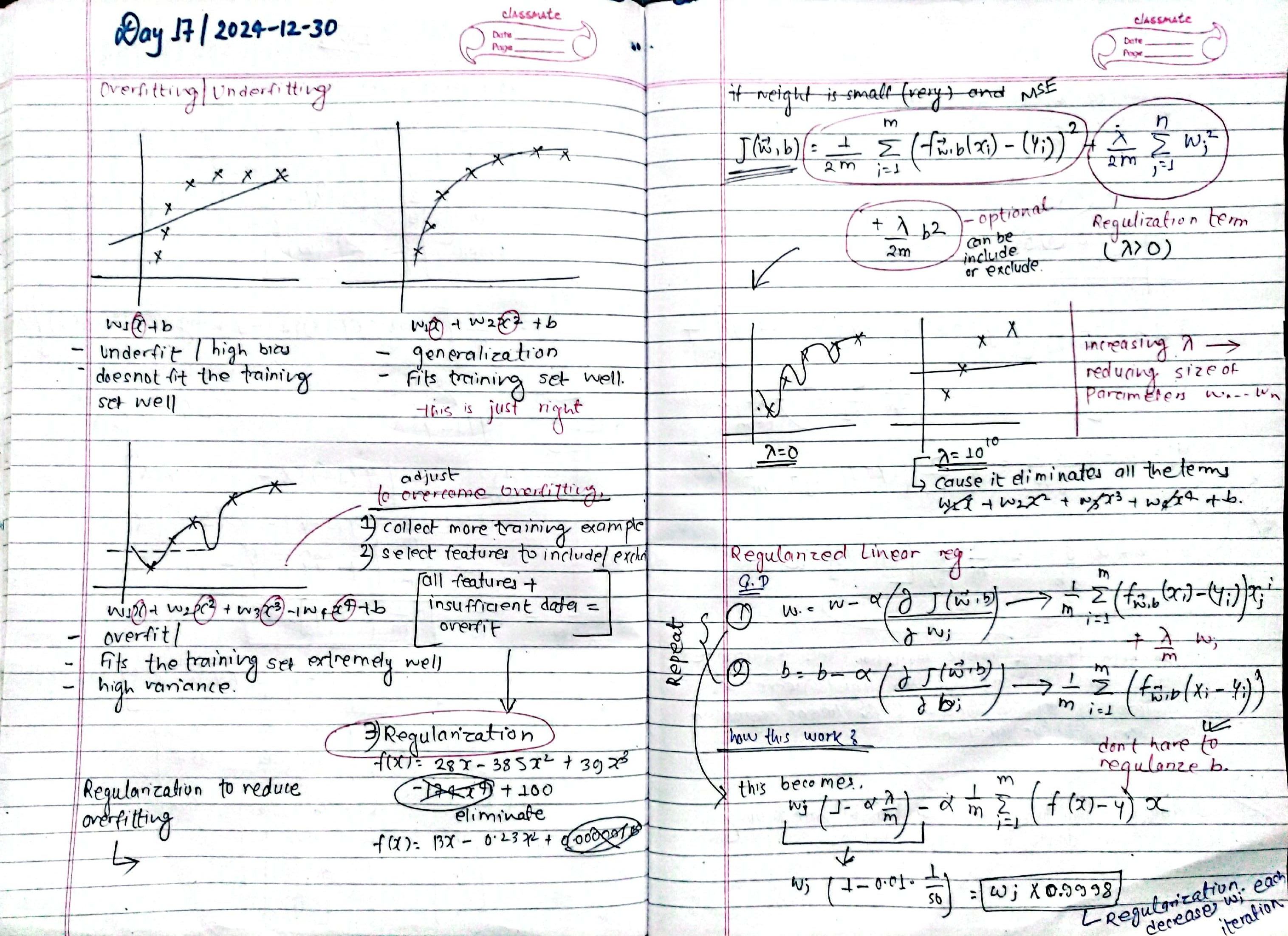
Day 17: Underfitting, Overfitting
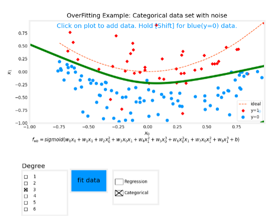
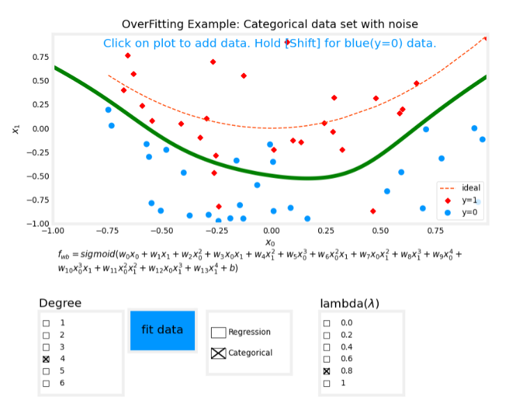
Today, explored teh concepts, overfitting (high variance), underfitting (high bias) and generalization(just right). Regularization to reduce Overfitting. Explored Regularized logistic regression.
- If the data is in non linear behaviour then we have to appply Ml algos like decision tree, random forest and svm.
Explored hypermeters of logistic regression, and gained some knowledge.
Day 18: Neurons, Layer, Neural netowrk, forward propagation
-
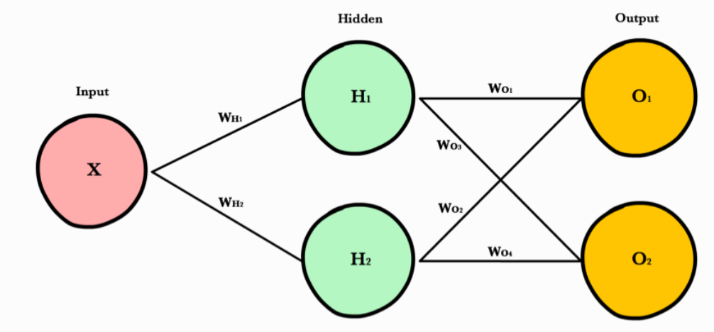
neural network: neural networks are machine learning algorithms that model complex patterns using multiple hidden layers and non-linear activation functions. they take inputs, pass them through hidden layers of neurons, and output a prediction.
-
Neurons: a neuron takes weighted inputs, applies an activation function, and outputs a result. inputs can be features or outputs from previous neurons, with weights adjusting their influence.
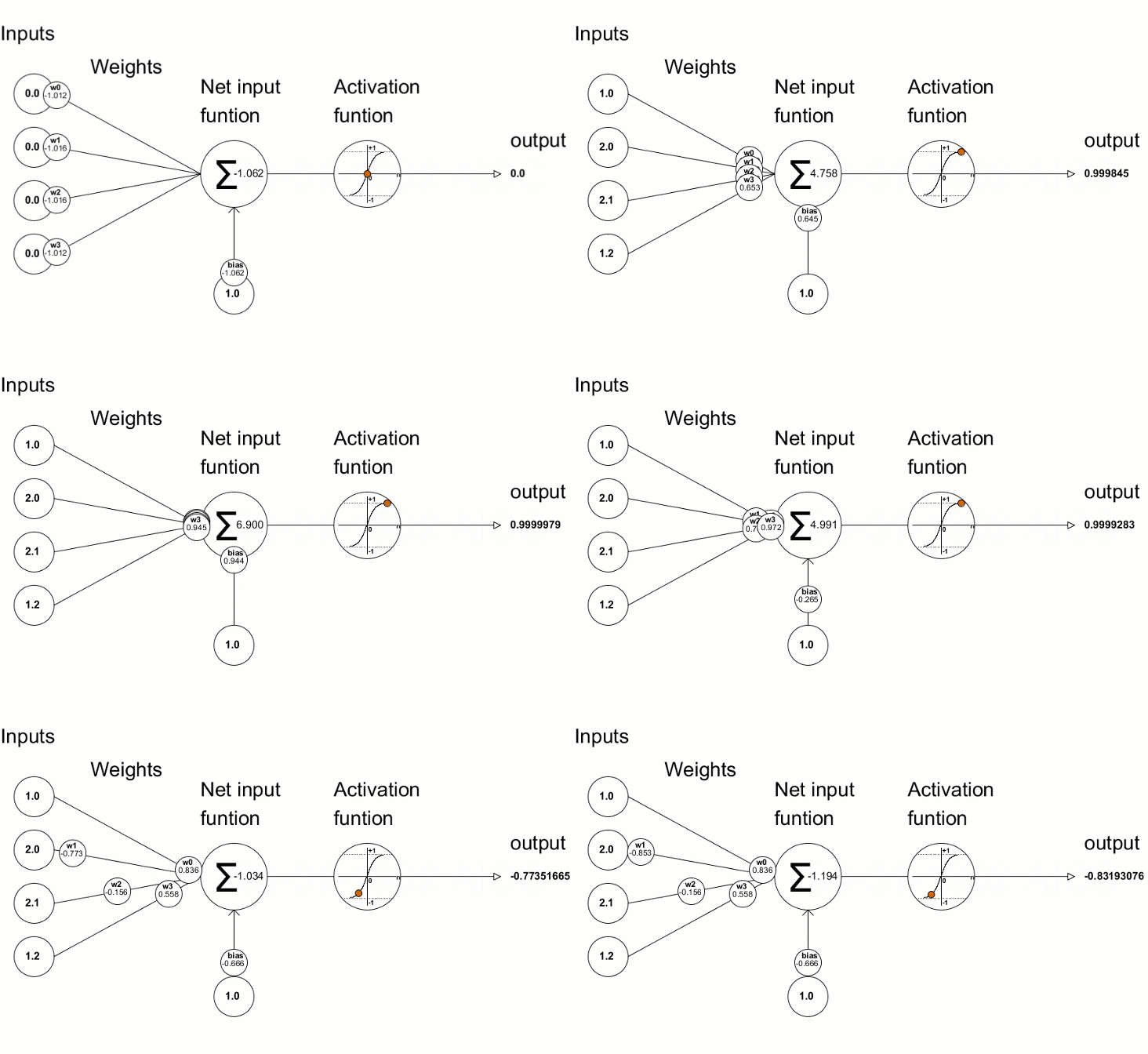 fig: single neuron in action
 -
Synapse: synapses connect neurons and carry the weighted inputs. each connection has a weight that adjusts during training.
-
weights: weights control the strength of connections between neurons. they are multiplied by inputs to influence the output, and are adjusted during training.
Popular activation functions include relu and sigmoid.
-
Bias: bias is a constant added to the weighted input before applying the activation function, helping the model represent patterns that don’t pass through the origin.
-
Layers:
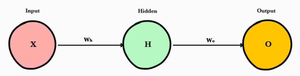
- input layer: holds the data for the model, with each neuron representing an attribute.
- hidden layer: applies activation functions to the inputs and passes results to the next layer.
- output layer: receives input from the last hidden layer and returns the model’s prediction.
Day 19: Forward Propagation
- Forward Propagation: Input data is “forward propagated” through the network layer by layer to the final layer which outputs a prediction.
Notes for today:
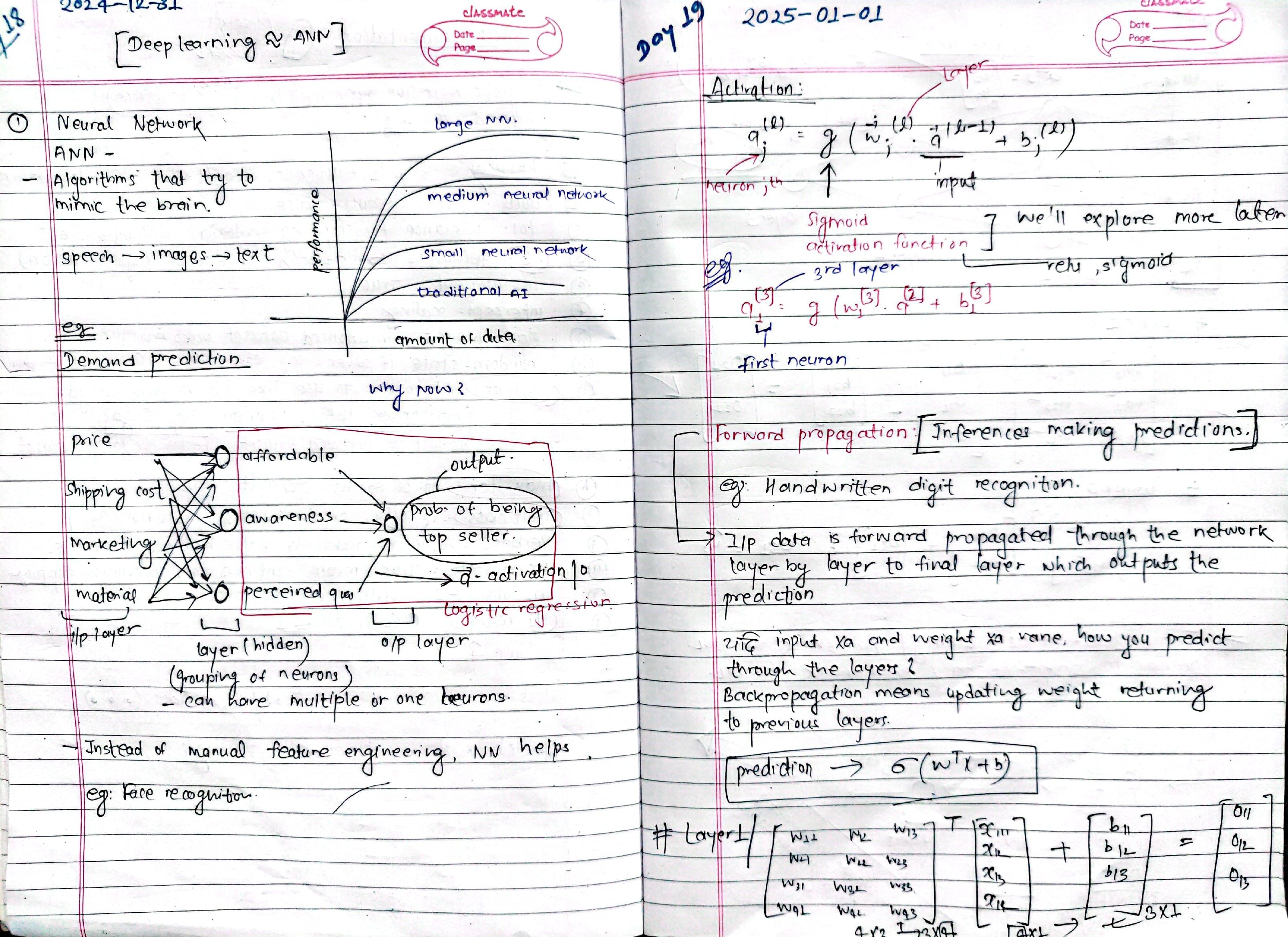
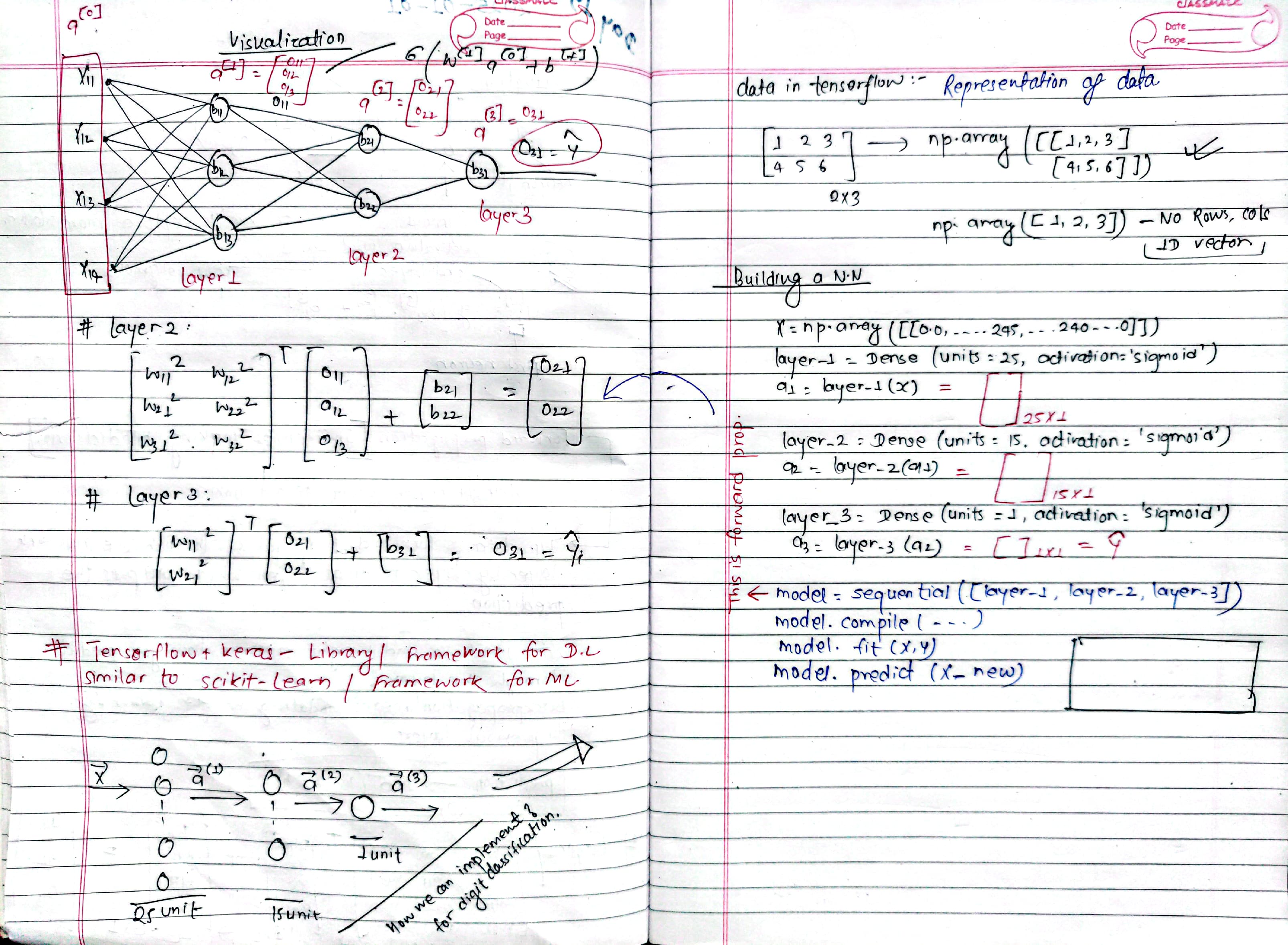
Matrix Representation:
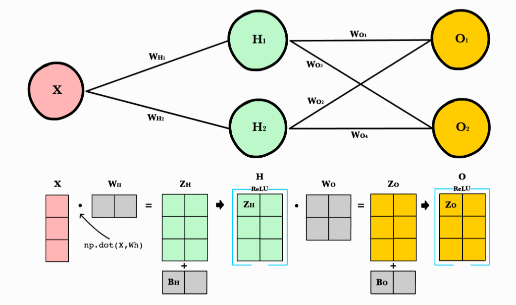 How forward Prop works for digit classification??
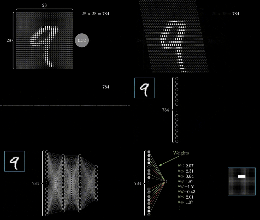 Notebook: Neurons and Layers
Notebook: A small Neural Netowrk using tensoflow
Notebook: Neurons and Layers
Notebook: A small Neural Netowrk using tensoflow
- tensorflow basics:
-
representation of data:numpy arrays used for input (e.g., 2D arrays).
x = np.array([[1, 2, 3], [4, 5, 6]]) -
building a neural network:
-
define layers:
layer1 = dense(units=25, activation='sigmoid') layer2 = dense(units=15, activation='sigmoid') layer3 = dense(units=1, activation='sigmoid') -
stack layers in a model:
model = sequential([layer1, layer2, layer3]) -
compile and train:
model.compile(optimizer='adam', loss='binary_crossentropy')
model.fit(x, y, epochs=10)
-
-
visualization:neurons connect layer by layer, with weights and biases computed at each step (refer to attached gif).
-
Day 20: Python Implementation from Scratch
Implemented forward propagation to compute predictions and backpropagation to optimize weights for binary classification.
- AGI: An advanced AI capable of generalizing across tasks like humans.
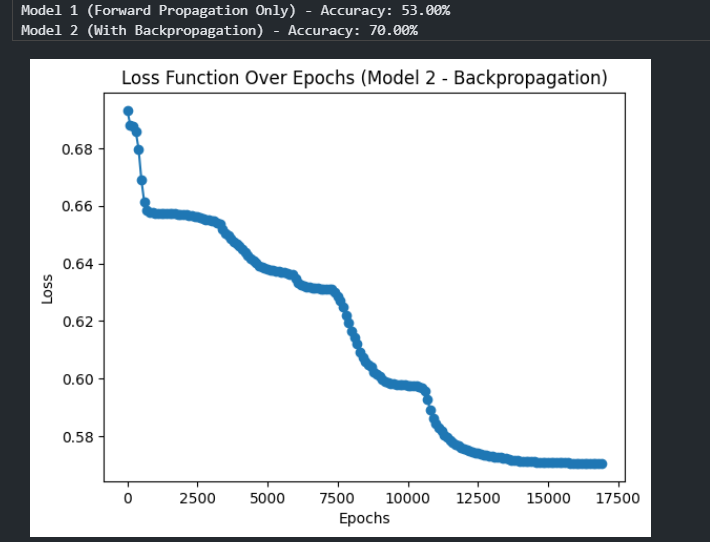
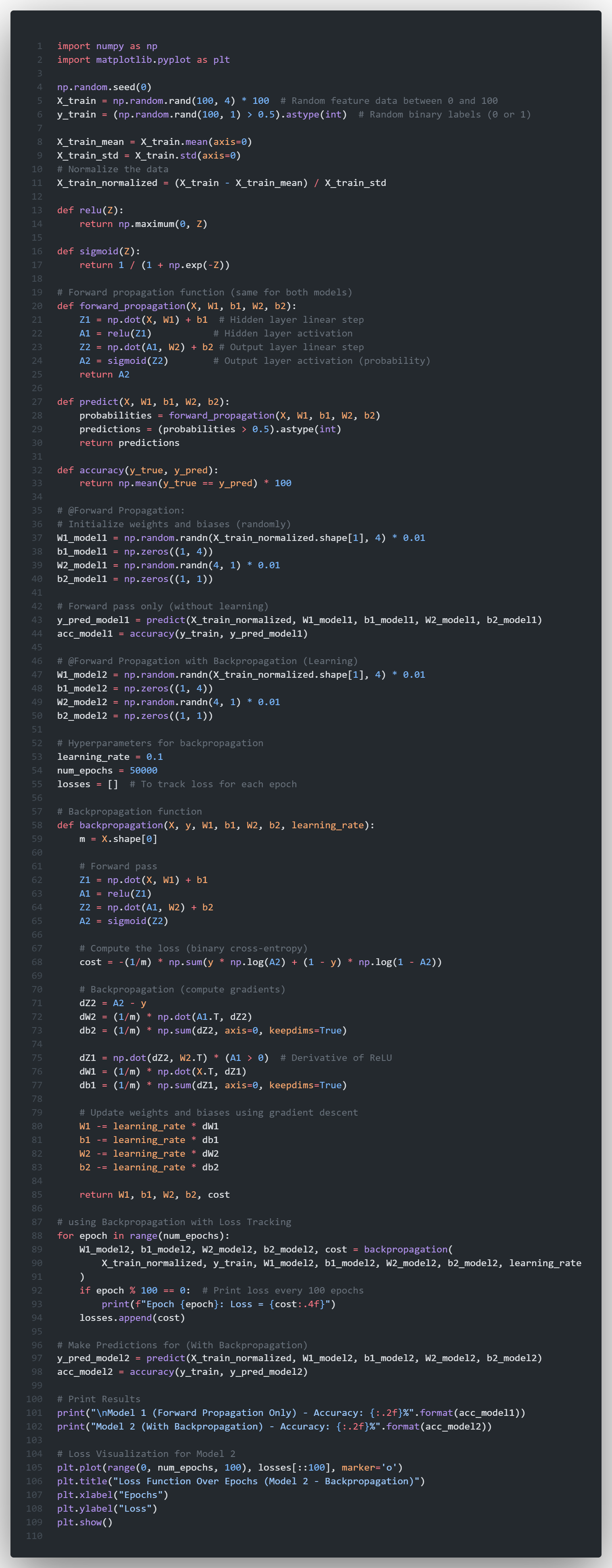
Day 21: Vectorization, Model Training
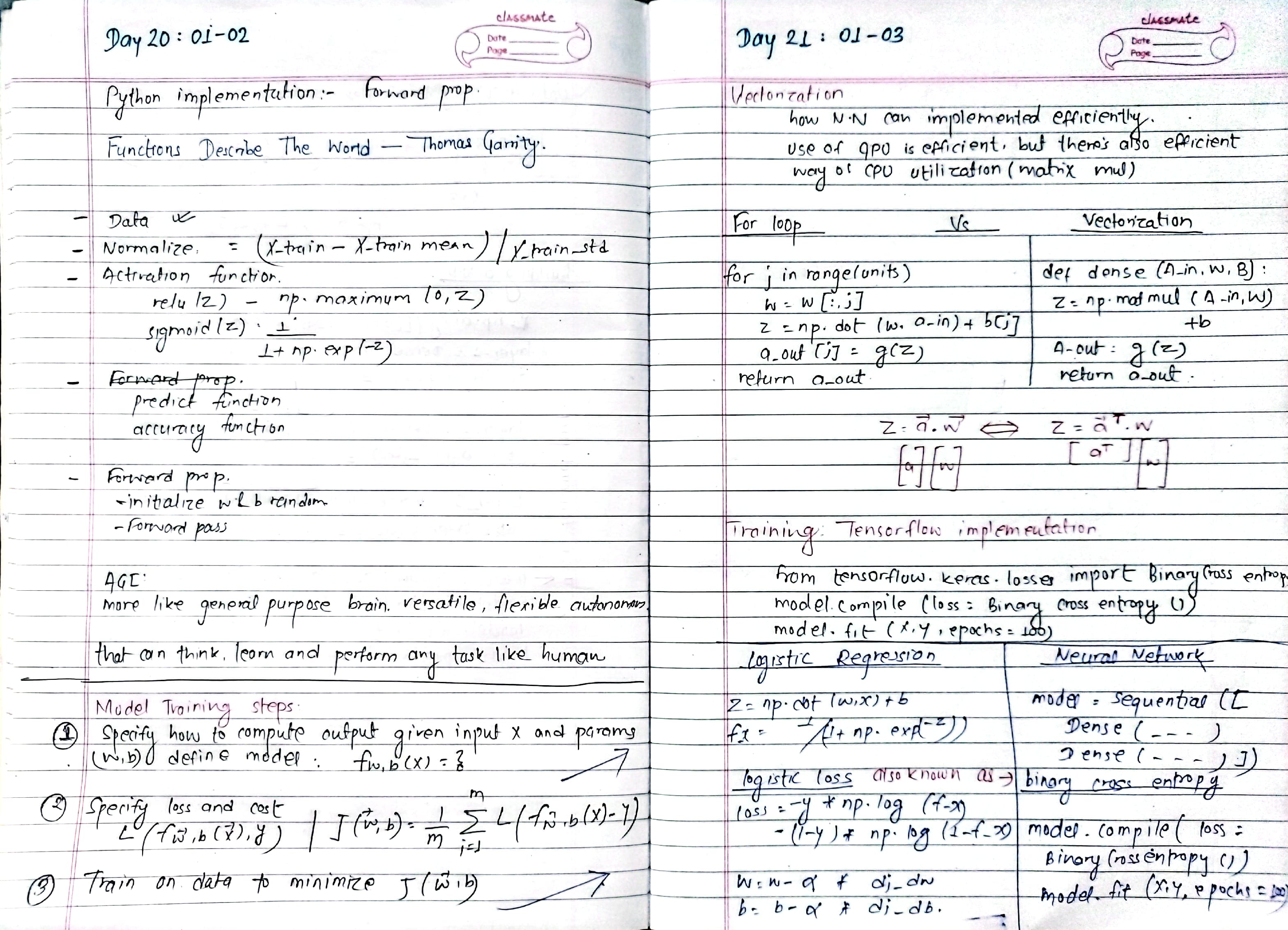
Exploredd Vectorization for efficient computation
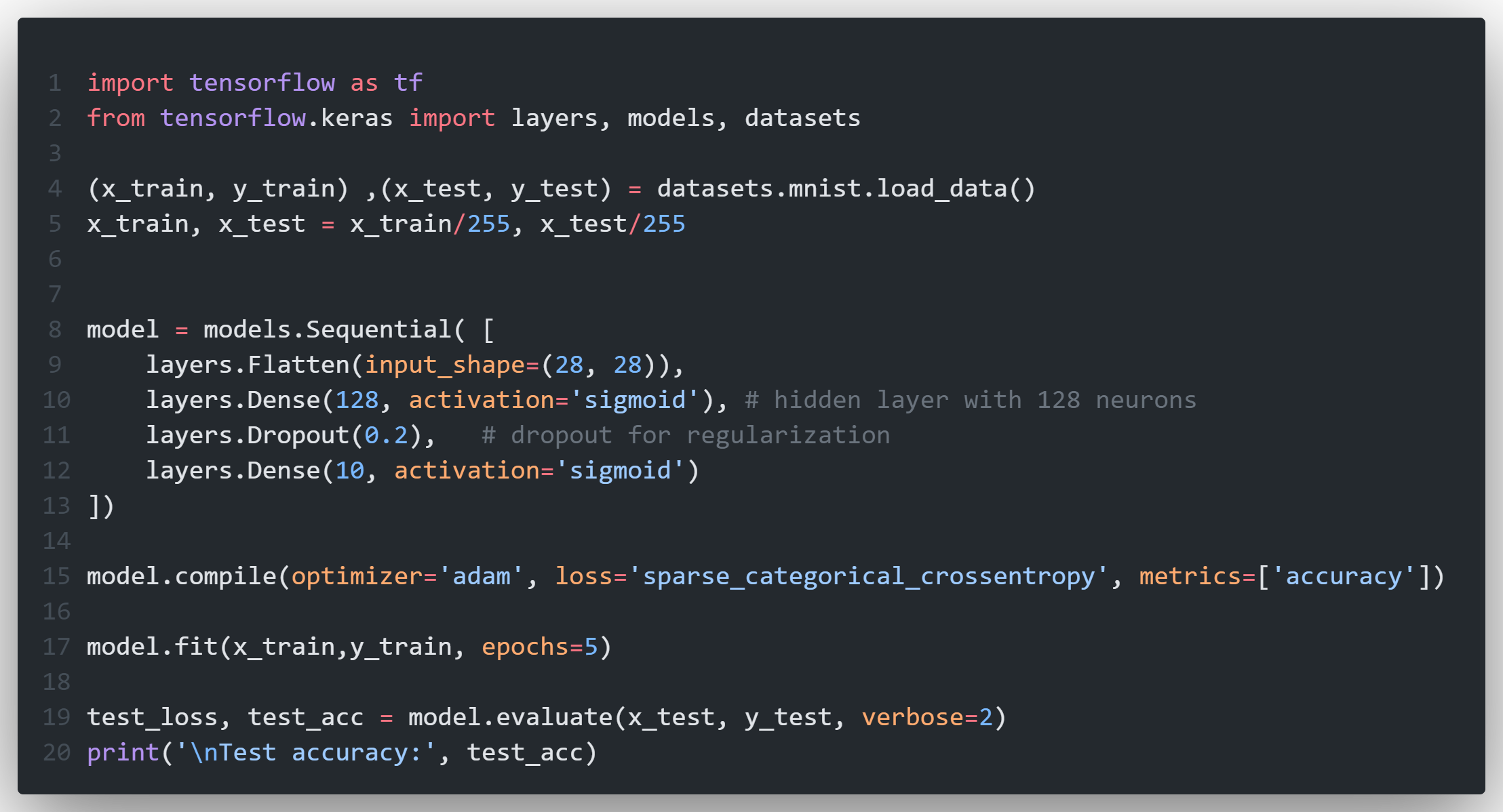
- Tensorflow: model.compile, binary_crossentropy, model.fit trained a binary classification model and tested its accuracy
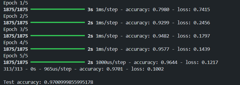 Training Model with tensorflow:
 Notes for today:
Day 22: Activation Functions, Softmax
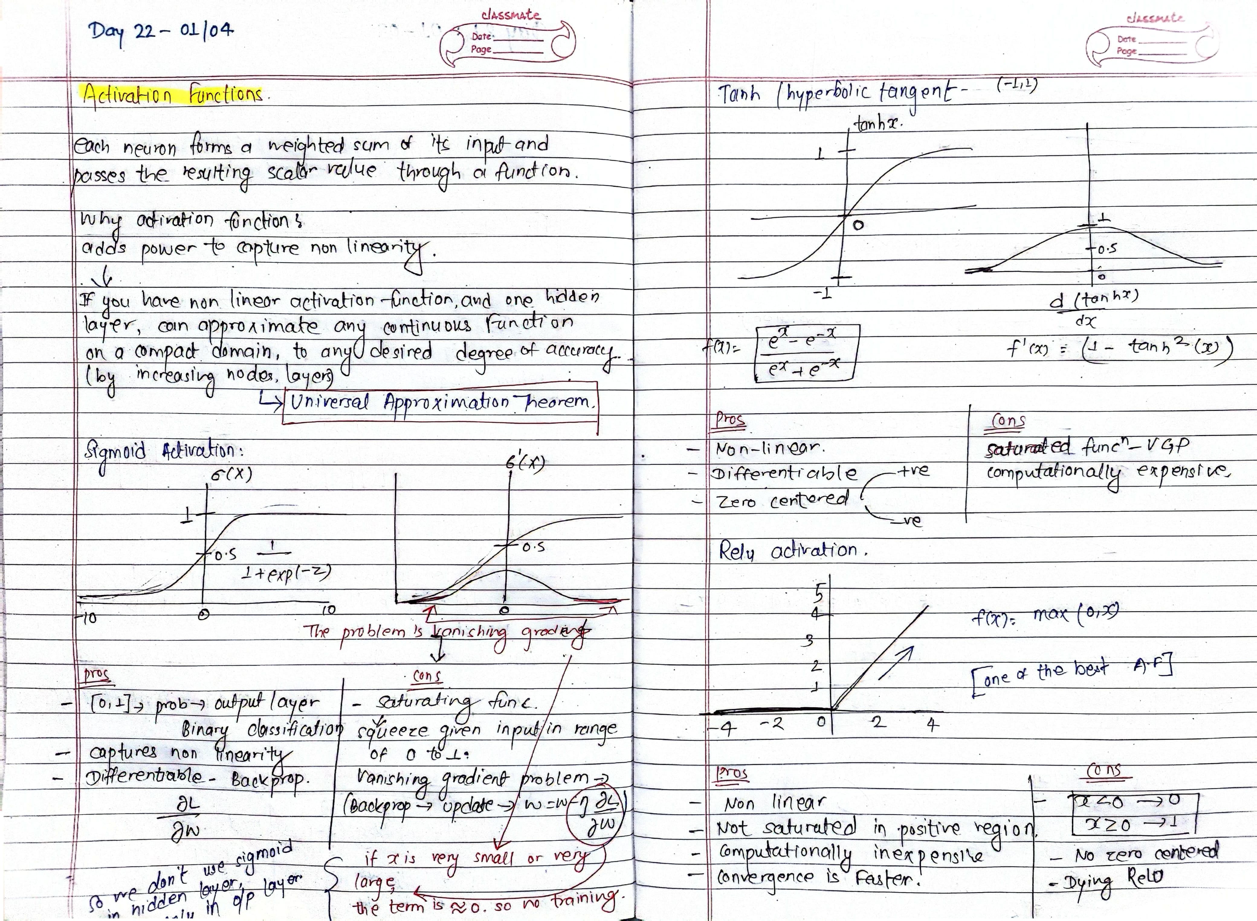
the universal approximation theorem explains that a neural network with enough hidden neurons and non-linear activations like sigmoid or relu can approximate almost any function, even complex patterns like wavy graphs.
Activation Functions:
commonly used activation functions include:
- sigmoid: squashes values between 0 and 1, often used for binary classification.
- relu: outputs 0 for negatives and the input itself for positives, commonly used in hidden layers.
- tanh: outputs between -1 and 1, useful for centered data.
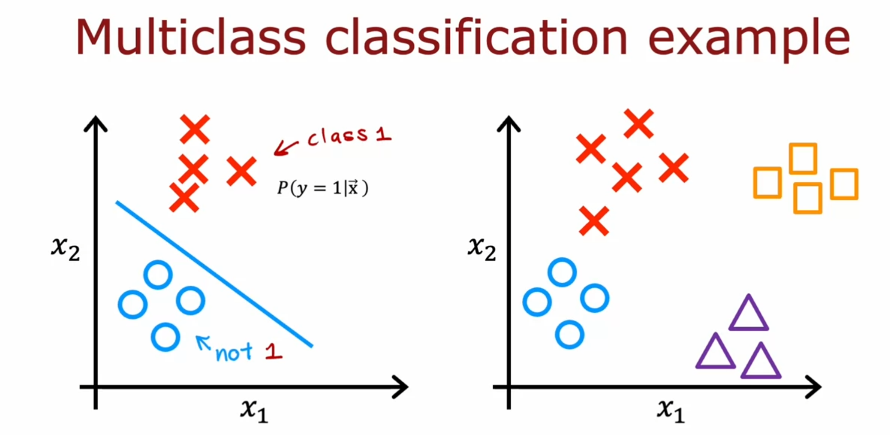
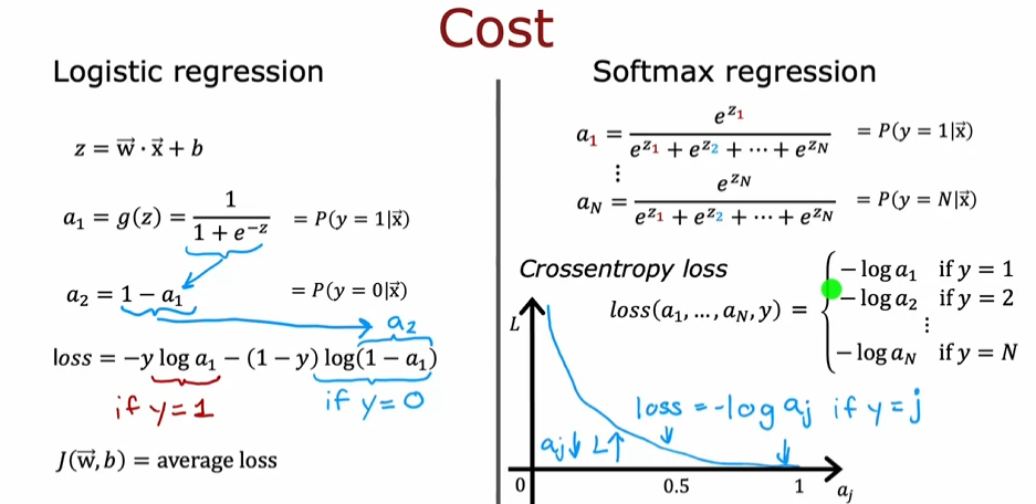
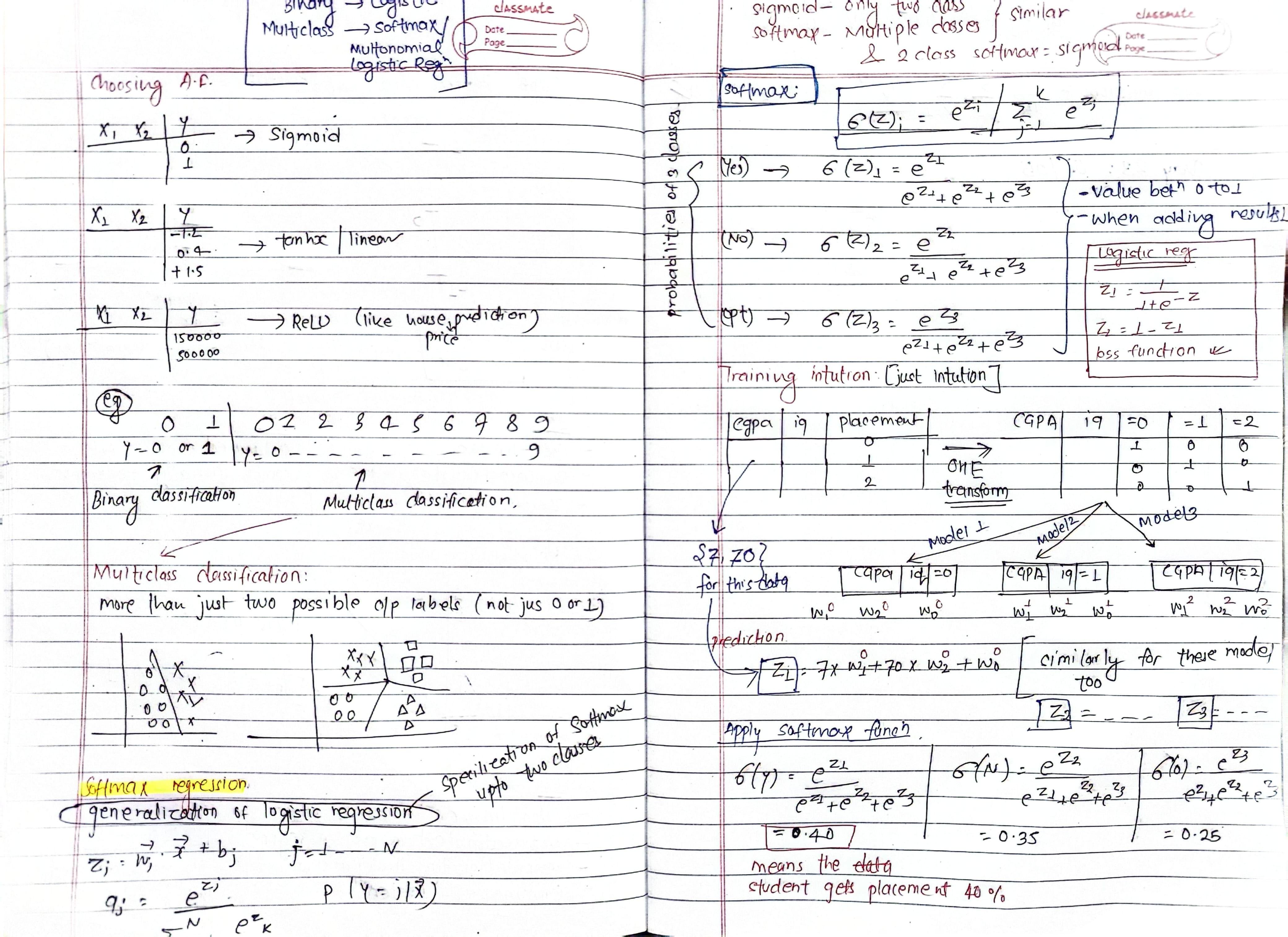
for multiclass classification, softmax is ideal in the output layer as it converts logits into probabilities that sum to 1. during training, the model adjusts weights to maximize the correct class probability, using categorical cross-entropy loss. softmax generalizes logistic regression, which is typically used for binary classification. in both, activation and loss functions differ based on the output type.
Logistic Vs softmax:
Notes:
Day 23: Implementation of Softmax Regression
- Classification with multiple Outputs: PS: there's difference between multiclass classificaiton and multilabel classification Notebook: Softmax/Multinomial in Iris dataset- Multilabel
NOTE: softmax regression is a classification algorithm that calculates probabilities for multiple classes using a linear combination of inputs and the softmax function. the class with the highest probability is chosen as the prediction
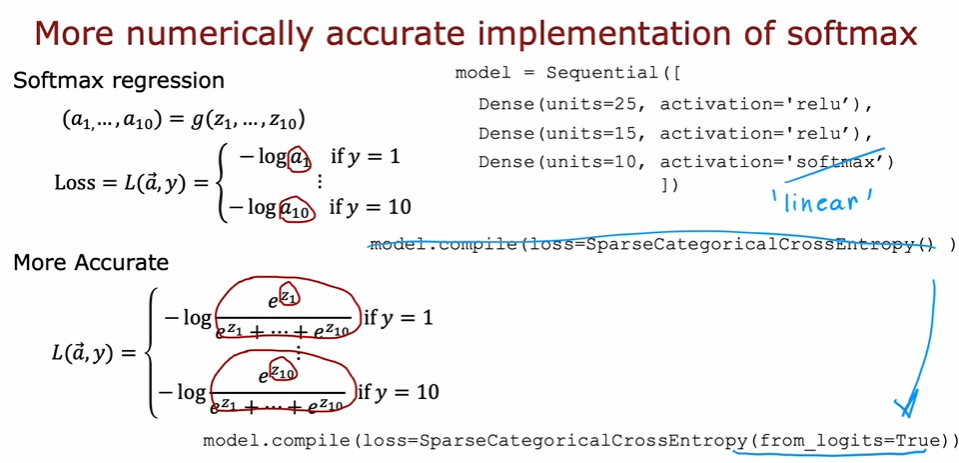
Improved Implementation of Softmax:
Tensorflow implementation:
model = Sequential(
    [
        Dense(25, activation = 'relu'),
        Dense(15, activation = 'relu'),
        Dense(4, activation = 'softmax')    # < softmax activation here

        ##         Dense(4, activation = 'linear')   #<-- Note
    ]
)
model.compile(
    loss=tf.keras.losses.SparseCategoricalCrossentropy(),
    ##     loss=tf.keras.losses.SparseCategoricalCrossentropy(from_logits=True),  #<-- Note ---- This is preferred model softmax and loss are combined for more accurate result.
    optimizer=tf.keras.optimizers.Adam(0.001),
)

model.fit(
    X_train,y_train,
    epochs=10
)
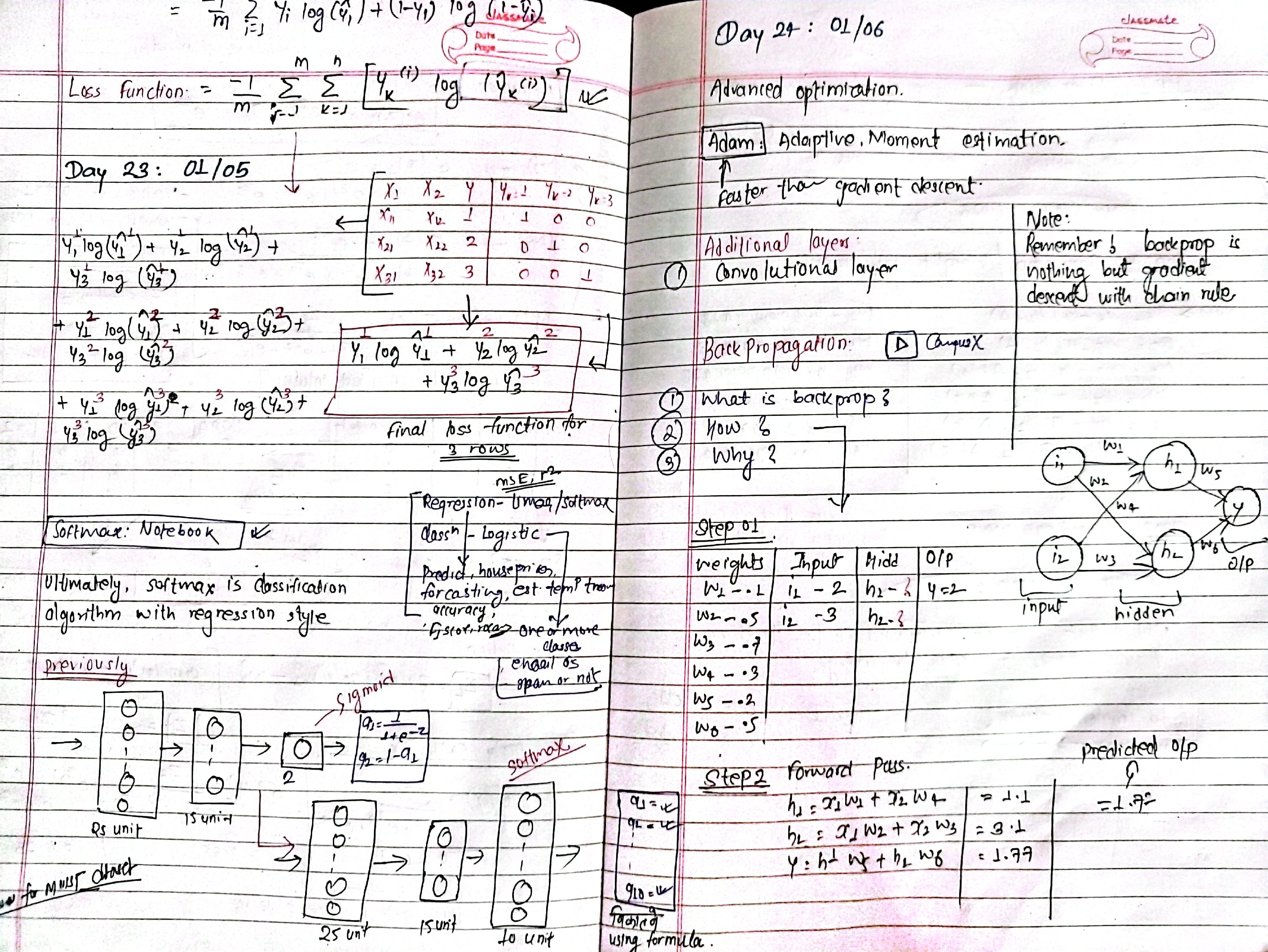
Day 24: Backpropagation - what and how ?
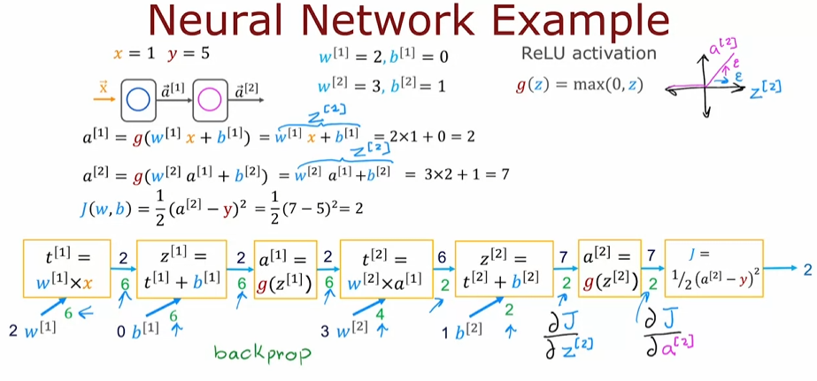
- what? Backpropagation adjusts nneural network weights by propagating errors backward using the chain rule and optimizing them with gradient descent.
- how? Forward pass to compute outputs, Calculate errors, propagate them backward, and update weights iteratively. Take a look at document below.
Backpropagation example with Neural Network:
Notes:
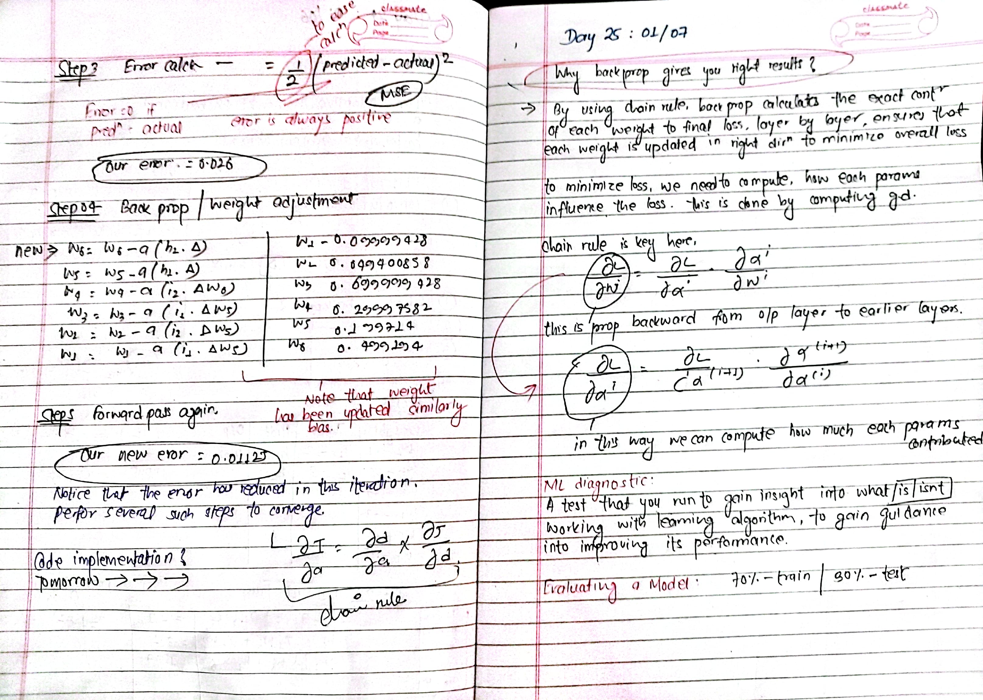
Day 25: Backpropagation - Why? Advices for applying machine Learning
Today, I dived into the reasons behind backpropagation's effectiveness in training neural networks. It's not just about adjusting weights; it's the gradients that guide optimization, helping the model minimize error and improve predictions. The backpropagation process makes sure that the error gets distributed in a way that leads to better learning.
How????
- Gradients: they ensure efficient error minimization by guiding weight updates.
- Optimization: properly tuned gradients lead to smoother optimization and faster convergence.
- Model Evaluation: evaluating model performance becomes easier with backpropagation because of the systematic error propagation and weight adjustments.
Notes:
Day 26: Model selection and training/cross validation/test sets, Bias and Variance
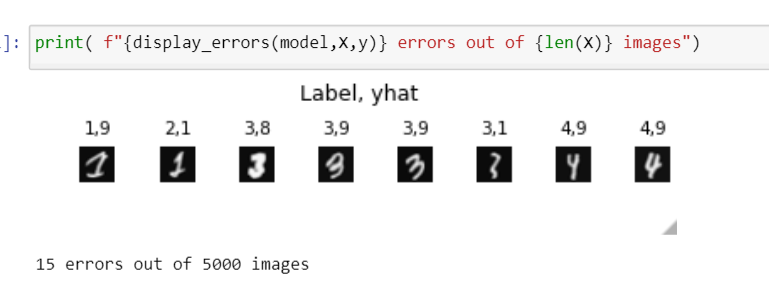
mnist dataset: Label and our prediction after training
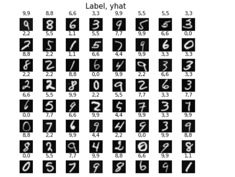 Errors in our prediction:
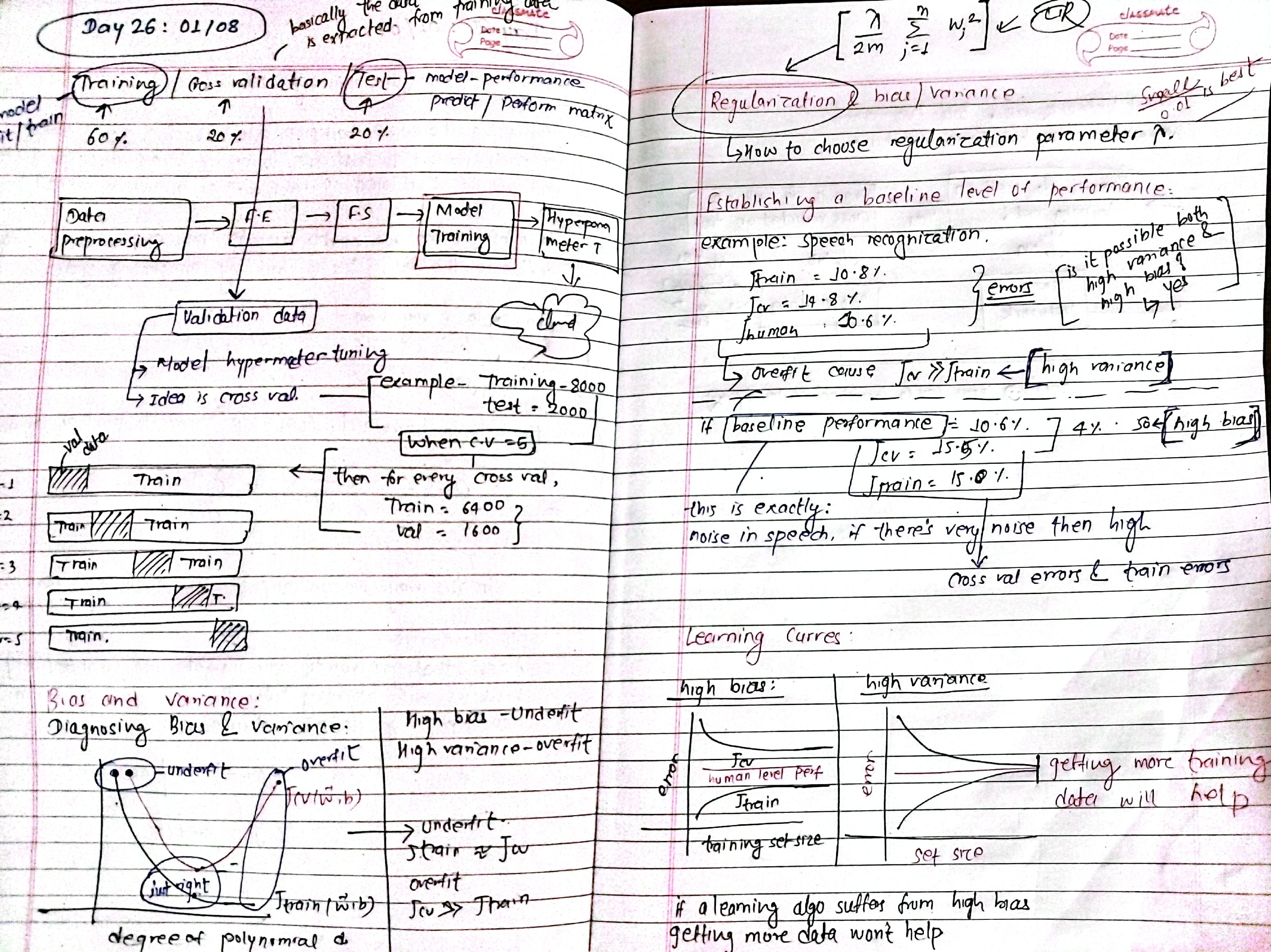
- the importance of splitting data into training, validation, and test sets cross-validation and its role in hyperparameter tuning.
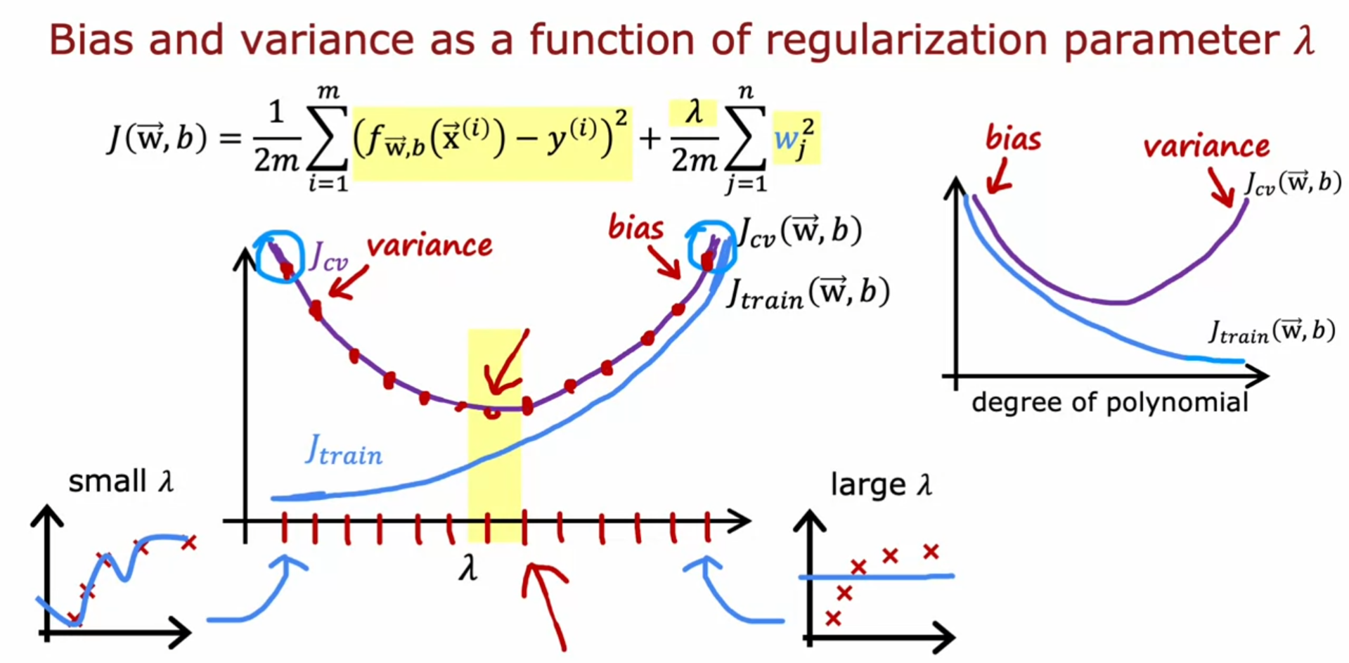
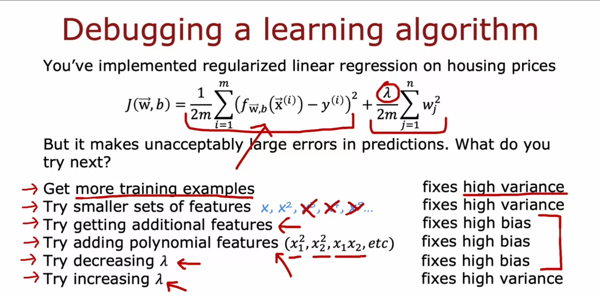
- Diagnosing bias and variance with error trends: high bias = underfit, high variance = overfit.
- regulariaztion to handle the tradeoff between bias and variance.
- how learning curves reveal insights about model performance and whether gathering more data will help.
Notes:
Notebook: Practice Lab: Neural Networks for Handwritten Digit Recognition, Multiclass
Notebook: Diagnosing Bias and Variance
Notebook: Model Evaluation and selection
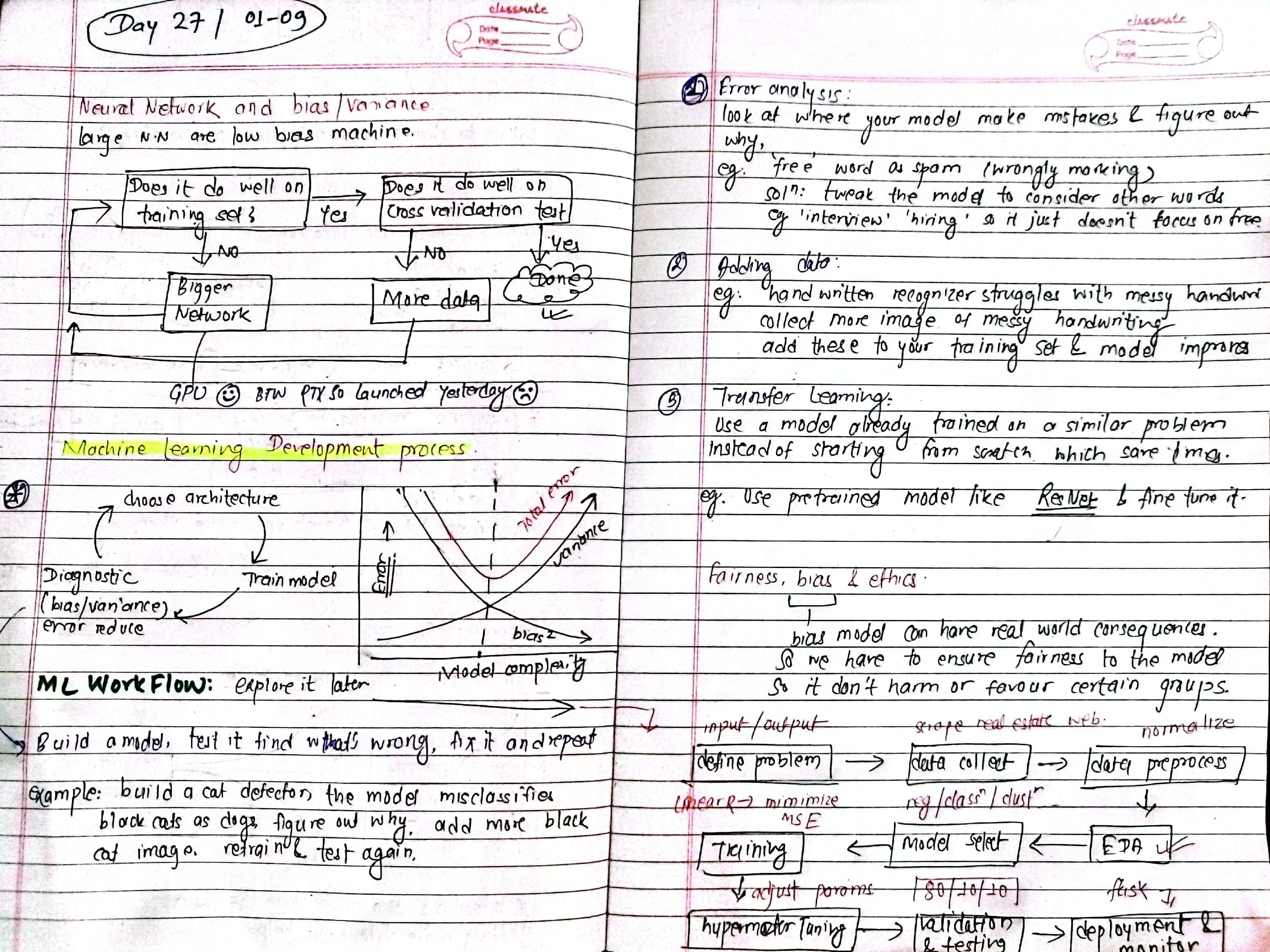
Day 27: Machine Learning Development Process, ML workflow
machine learning development process
- ml development is iterative, involving:
- choosing model and data architecture.
- training the model.
- diagnosing bias, variance, and errors.
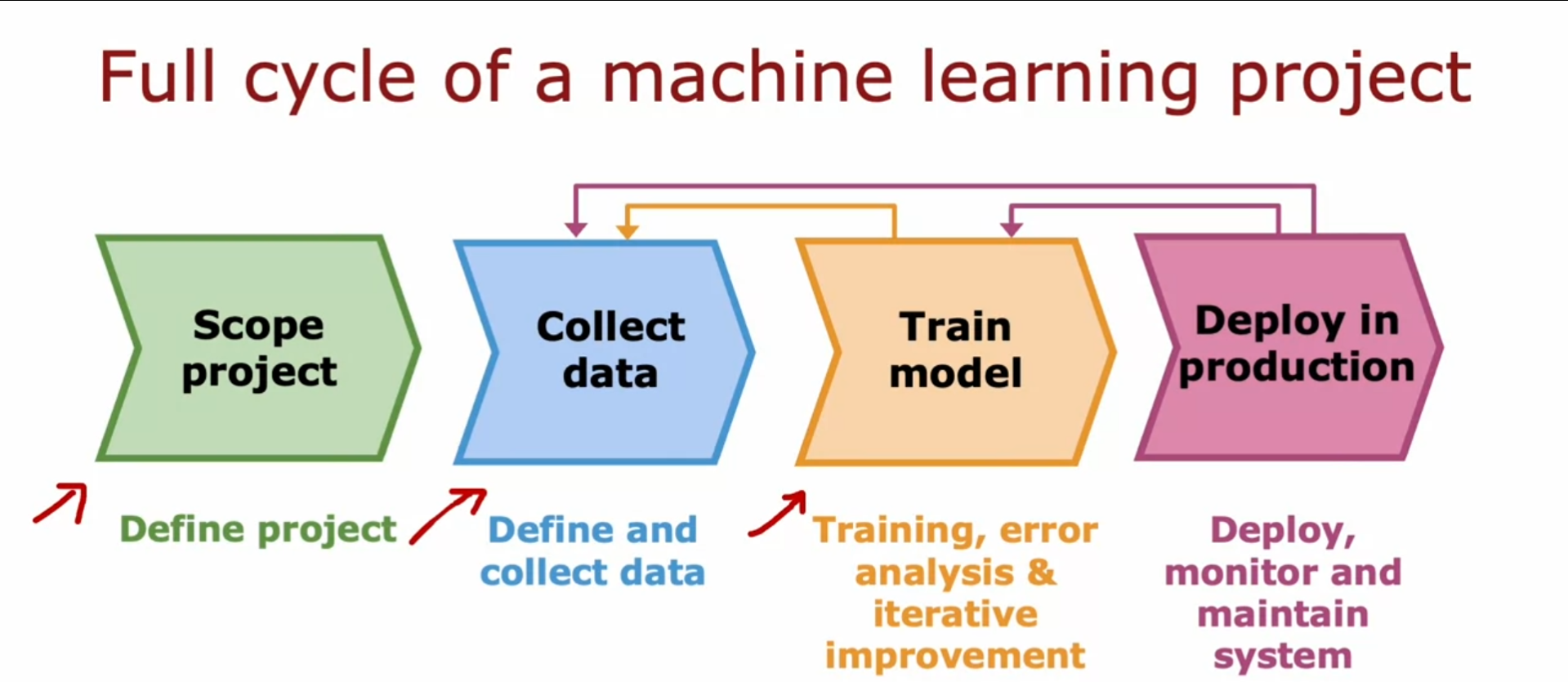 2. error analysis: identify and fix patterns in model failures.
3. adding data:
- data augmentation: modify existing data (e.g., distortions).
- data synthesis: create artificial data.
-
transfer learning:
- reuse pre-trained models for similar tasks.
- fine-tune them with your own data.
-
ml projects follow these steps:
- data collection.
- preprocessing.
- modeling.
- evaluation.
- deployment.
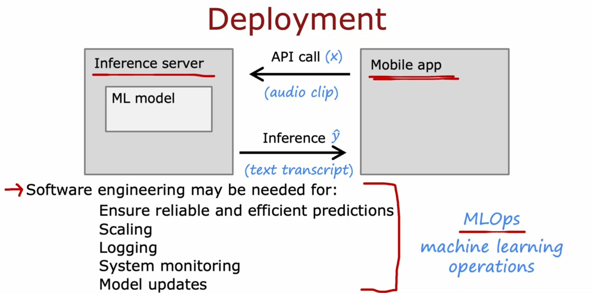
- monitoring.
-
ethics and fairness -
ensure ethical use by:- avoiding biased decisions in loans, jobs, etc.
- preventing harmful applications like deepfakes.
Notes:
Day 28: Machine Learning Model: Error Analysis and Transfer Learning
Notebook: Code Implementation from Scratch
-
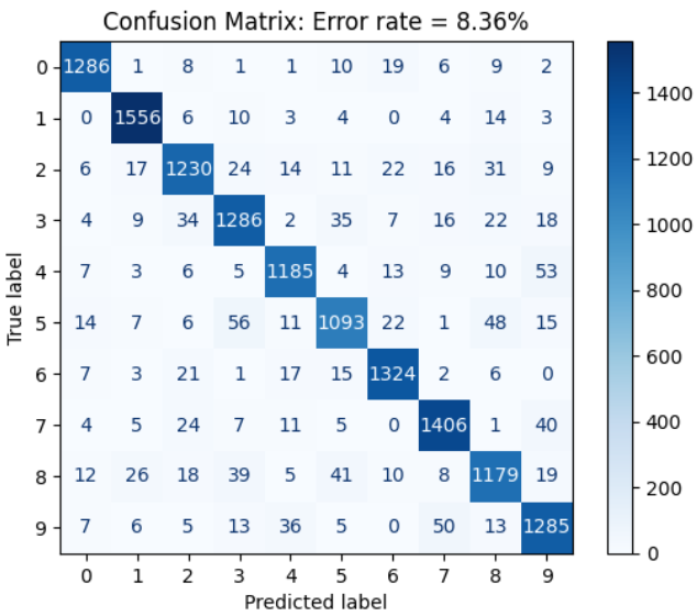
Confusion Matrix Analysis: the most frequent error is misclassifying 5 as 3. overall, the error rate is around 8%.
-
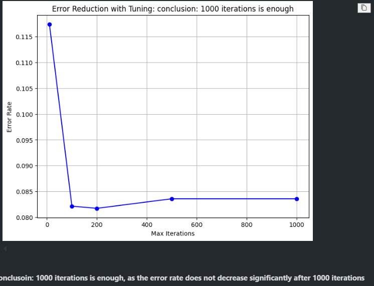
Iterations Insight: after 200 iterations, the error rate does not decrease significantly, suggesting that 200 iterations are enough for the model to converge.
-
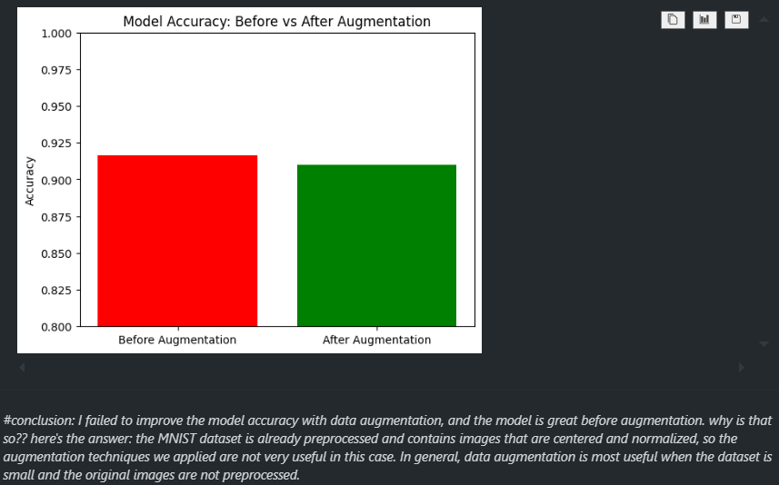
Data Augmentation Insight: despite applying data augmentation, there was no improvement in accuracy. this is because the MNIST dataset is already preprocessed, with centered and normalized images, making the augmentation techniques less effective. in general, data augmentation works best when the dataset is smaller or images are not preprocessed.
-
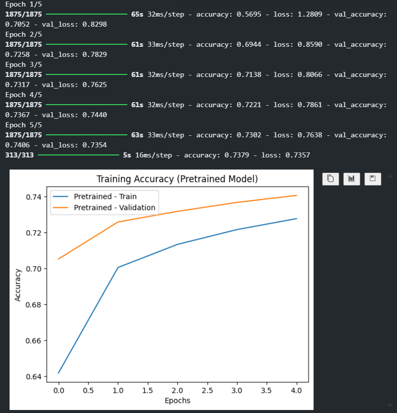
Transfer Learning with MobileNetV2:
- Training set accuracy improved from 56.95% to 73.02%.
- Validation accuracy increased from 70.52% to 74.06%.
- Loss decreased consistently for both training and validation sets, signaling better learning and generalization.
- The model shows significant improvement over epochs.
- Using transfer learning, the model started with an initial accuracy of 74% (pre-trained on ImageNet). As training progressed, the model continued to adapt, improving with each epoch. transfer learning was effective, yielding good results with fewer epochs.
Day 29: Error Metrices, Encoding of Categorical Data, Transoformers
Notebook: Lab week 3: Improving Model
Precision vs. Recall Trade-Off:
- High Precision: Only hire candidates you’re sure are good. Result: Fewer bad hires, but you might miss some great ones. Example: You hire 5 people, all are good, but you missed 10 other good ones.
- High Recall: Hire as many as possible to ensure no good candidate is missed. Result: You catch all great candidates but end up with some bad hires too. Example: You hire 50 people, 20 are good, but 30 are bad.
- When to Focus on Each?
-
Precision: When mistakes (bad hires) are costly. Example: Hiring a brain surgeon.
-
Recall: When missing good candidates is worse. Example: Hiring for a customer service team.
Encoding of Categoriical Data:
| Encoding Type | Use When | Example |
|---|---|---|
| Label Encoding | Small, unordered categories | Colors: [Red, Blue] |
| Ordinal Encoding | Ordered categories | Education: [Low, High] |
| One-Hot Encoding | Nominal data, fewer unique categories | Days: [Mon, Tue, Wed] |
Types of Transformers:
| Transformer | Purpose | Example Use Case | Input | Output |
|---|---|---|---|---|
| Column Transformer | Apply different transformations to different columns (e.g., scaling and encoding). | Scale age and one-hot encode city names. | Age: [25, 35, 45], City: [NY, LA, CHI] | [-1.22, 0, 0, 1], [0, 1, 0, 0], [1.22, 0, 1, 0] |
| Function Transformer | Apply a mathematical function (e.g., log or sqrt) to all values. | Apply logarithmic transformation to data. | [1, 10, 100] | [0.69, 2.39, 4.61] |
| Power Transformer | Normalize and reduce skewness in data, making it more Gaussian-like. | Stabilize variance in highly skewed data. | [1, 10, 100] | [-1.22, 0.0, 1.22] |
Day 30: Scikit-Learn Pipelines & Ridge Regression (L2 Regularization)
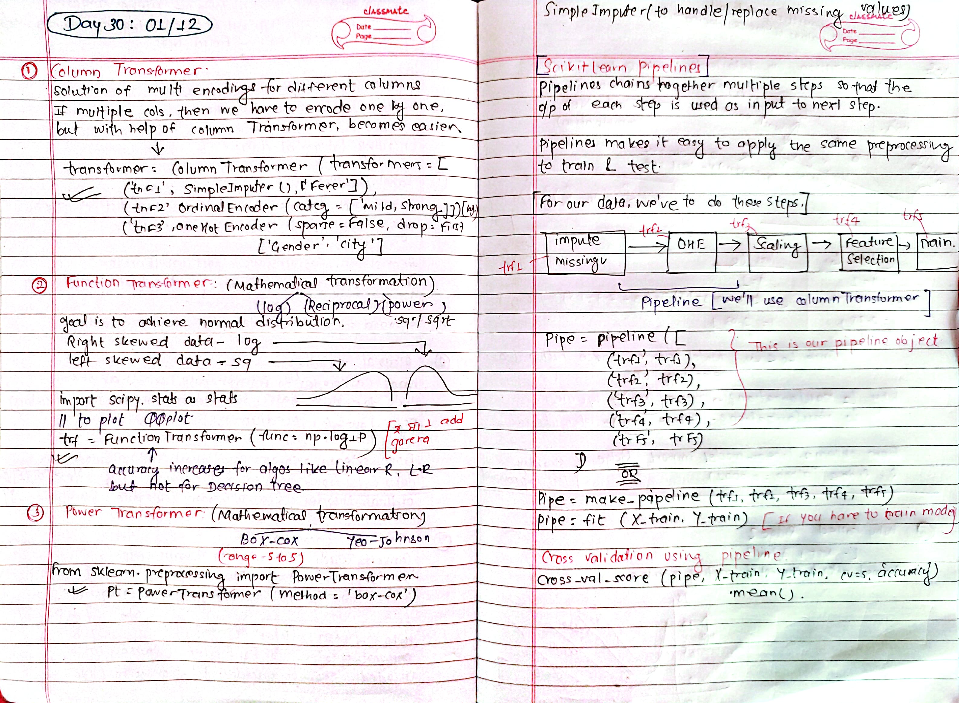
I explored how to create pipelines in Scikit-learn to streamline the process of combining multiple steps (like preprocessing, model fitting, and regularization) into a single object. This simplifies workflows and ensures reproducibility.
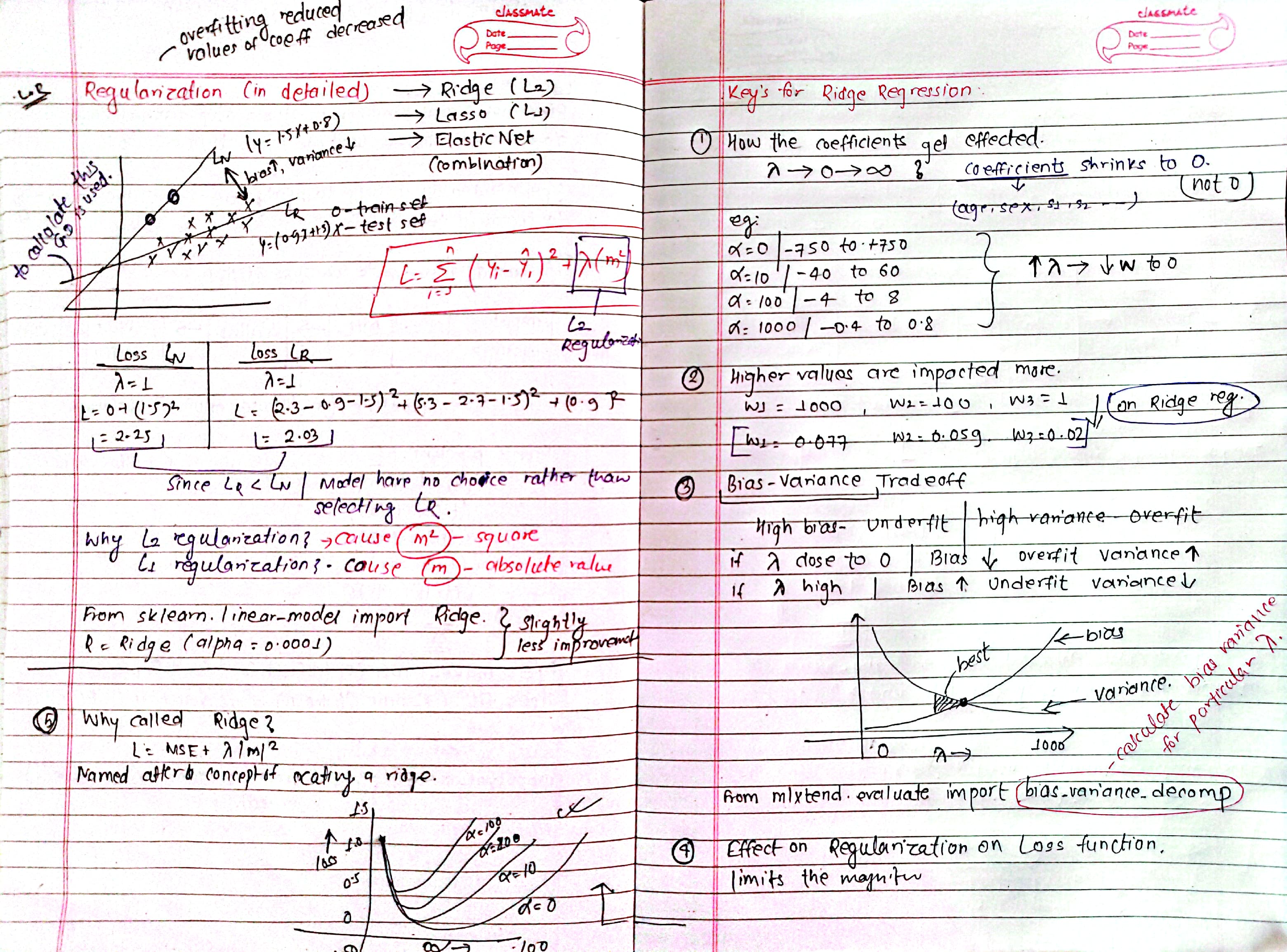
There are three techniques of regularization:
- Ridge (L2)
- Lasso (L1)
- Elastic Net (Combination)
Key Understanding of Ridge Regression:
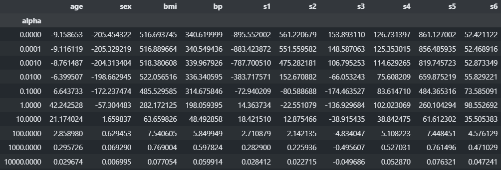
- How the coefficient Get affected?
- Regularization shrinks the coefficients, preventing them from becoming too large, which reduces overfitting.
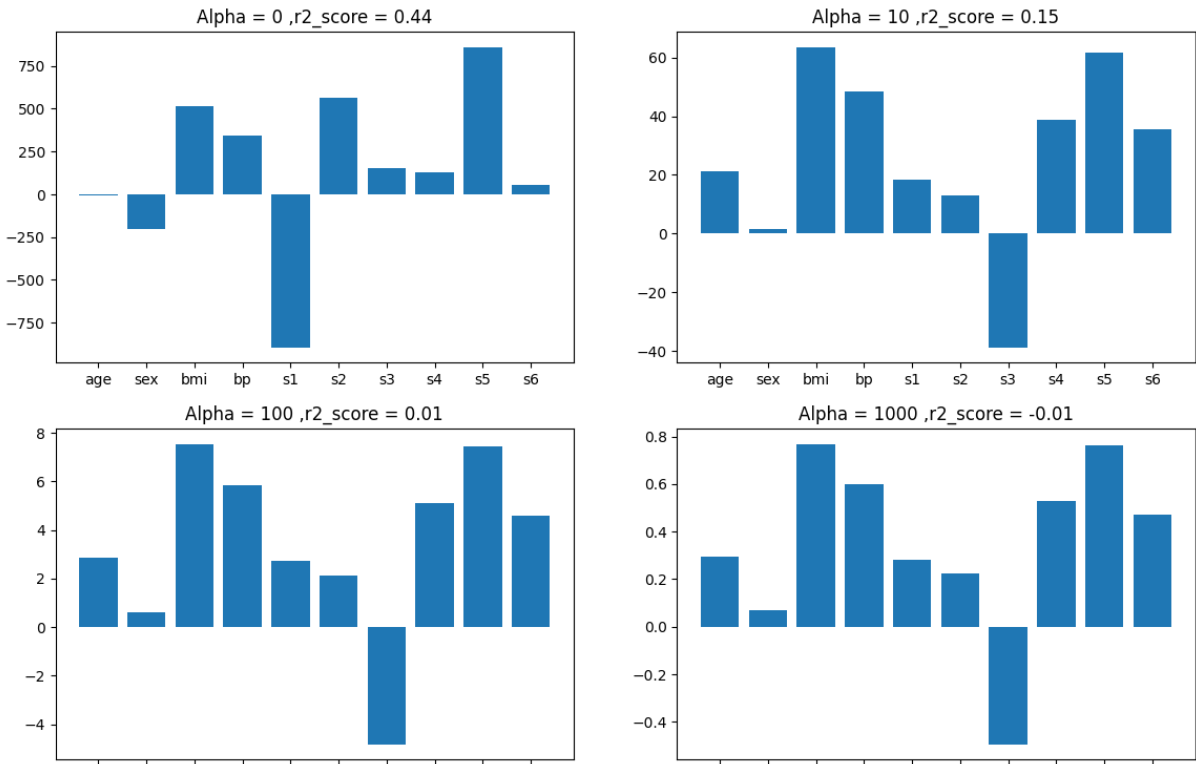
- Higher Values are impacted more
- The larger the regularization value (alpha), the more the coefficients are reduced.
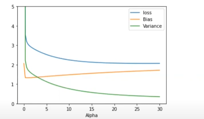
- Impact on Bias Variance Tradeoff
- Higher regularization increases bias but reduces variance, making the model more generalizable.
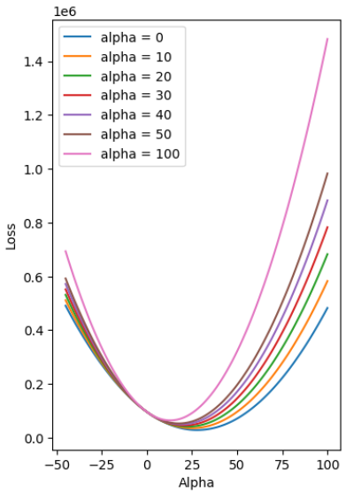
- Effect on Loss Function
- adds a penalty term that limits the magnitude of the coefficients.
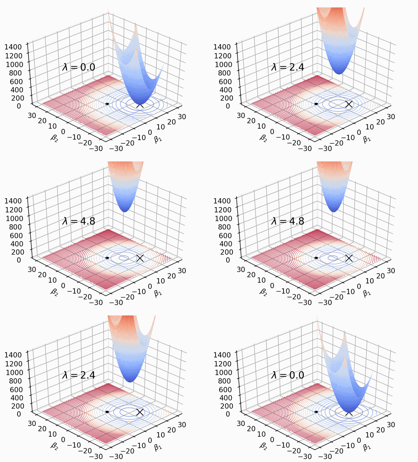
- Why Ridge Regression is called so?
- Named after the concept of creating a "ridge" or constraint on the model’s coefficients, preventing them from growing too large.
Notes:
Notebook: Key Understandings of ridge Regression
Day 31: Lasso Regression (L1 Regularization), Elastic Net Regularization
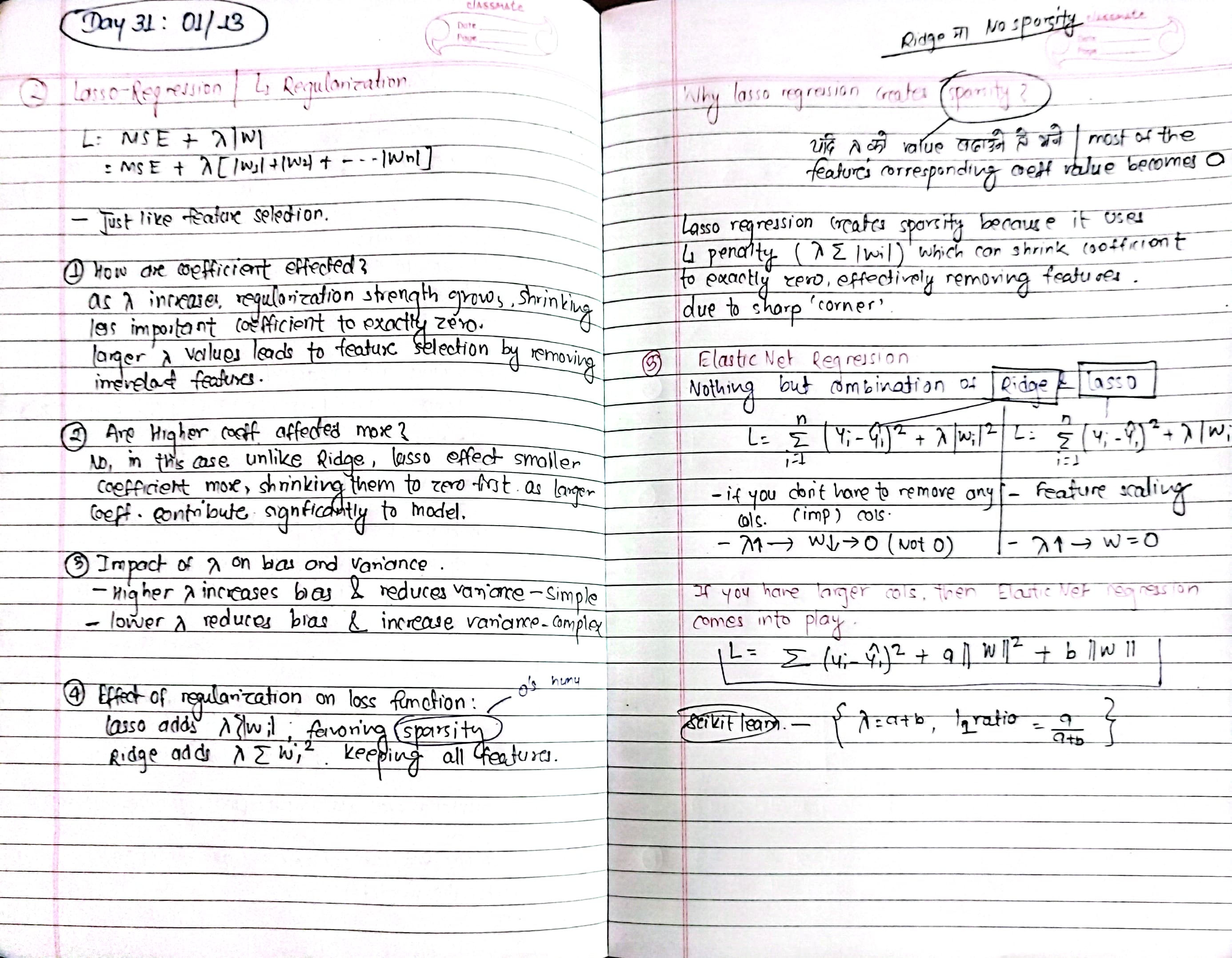
Lasso Regression:
-
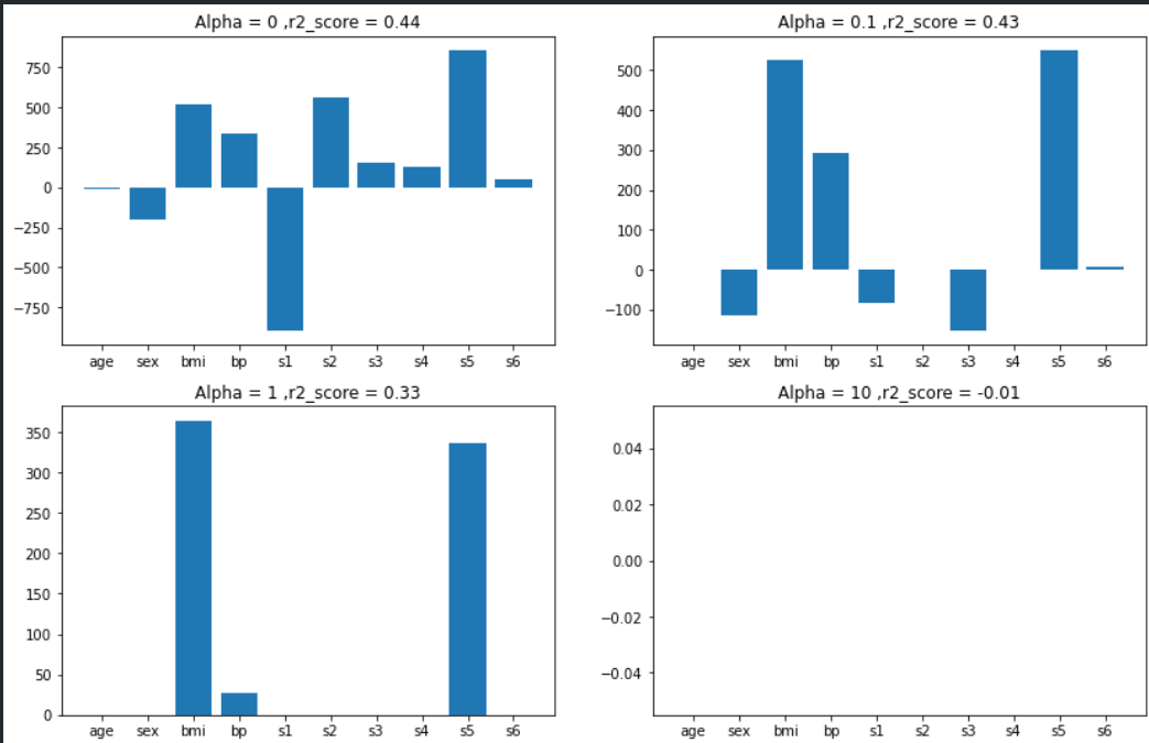
How are coefficients affected by λ (alpha)? As λ increases, regularization strength grows, shrinking less important coefficients to exactly zero. Larger λ values lead to feature selection by removing irrelevant features.
-
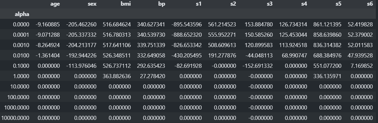
Are higher coefficients affected more? No. Lasso affects smaller coefficients more, shrinking them to zero first. Larger coefficients remain relatively unaffected if they contribute significantly to the model.
-
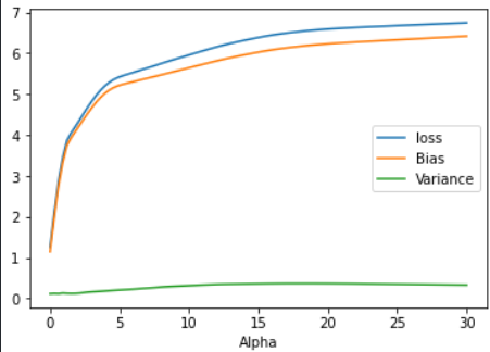
Impact of λ on bias and variance:
- Higher λ increases bias (simpler model) and reduces variance.
- Lower λ reduces bias (complex model) but increases variance.
-
Effect of Regularization on Loss Function:
- Lasso add λ sum(w_i) to the loss, promoting sparsity by penalizing the absolute magnitude of coefficients. Unlike Ridge, it can remove features entirely, improving interpretability.
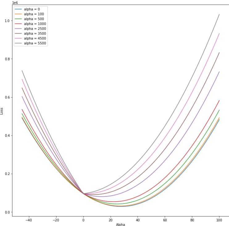
- Lasso add λ sum(w_i) to the loss, promoting sparsity by penalizing the absolute magnitude of coefficients. Unlike Ridge, it can remove features entirely, improving interpretability.
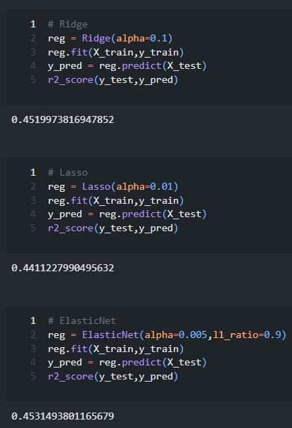
Elastic Net Regularization:
Elastic Net combines L1 (Lasso) and L2 (Ridge) penalties. It selects important features by shrinking some coefficients to zero (like Lasso) and handles correlated features by shrinking coefficients without setting them to zero (like Ridge). It’s useful when features are both highly correlated and some are irrelevant. Elastic Net is controlled by two parameters:
α (mix of Lasso and Ridge) and
λ (regularization strength).
Notes:
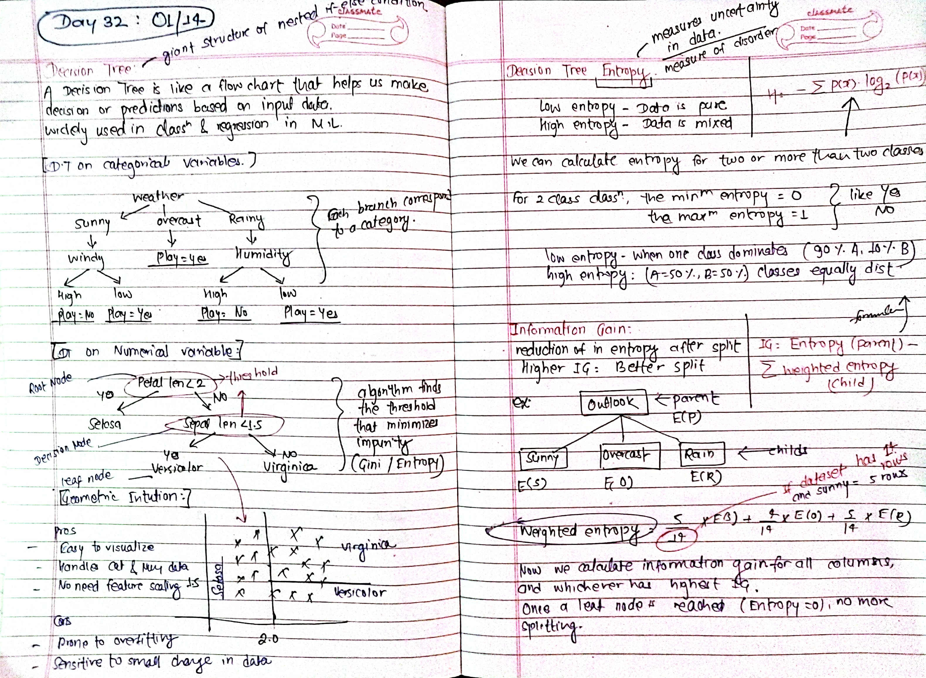
Day 32: Decision Tree: Entropy and Information Gain
A decision tree is a flowchart-like structure used for classification or regression, where data is split into branches based on conditions until a final decision (leaf) is reached.
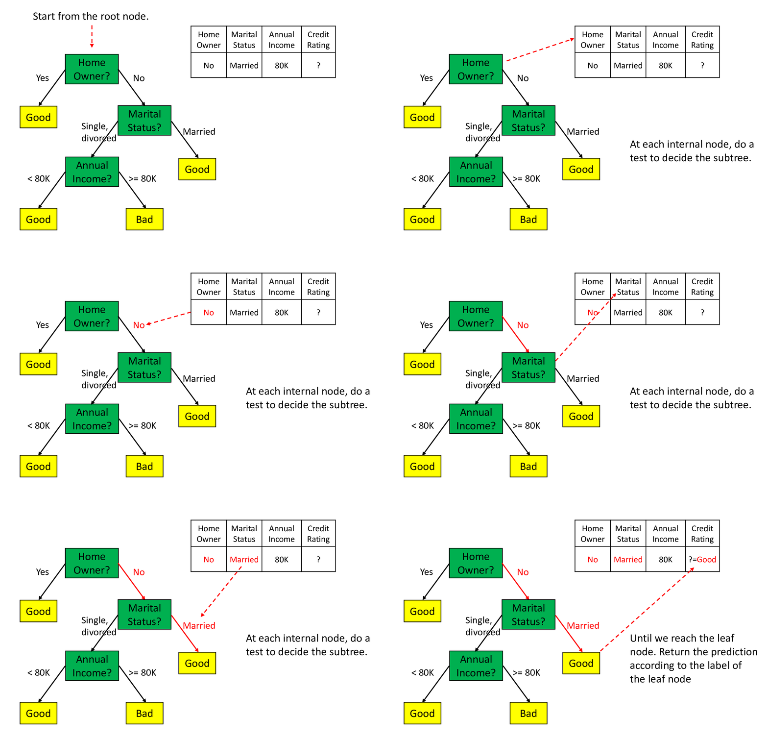
- Decision Tree on Categorical Variables: Splits data based on categories like "Sunny" or "Rainy".
- Decision Tree on Numerical Variables: Splits data using thresholds like Age > 30.
- How Decision Tree Works: Repeatedly splits data into smaller groups based on conditions.
- Terminology: Root (start), Branch (path), Leaf (decision).
- Pro - Simple to understand; Con - Can overfit.
- Entropy: Measures uncertainty; low entropy = purer data.
- Entropy Calculation:
∑ p(x) * log2(p(x)). - Information Gain: Reduction in entropy after splitting data.
IG=Entropy(before)−Weighted Entropy(after) - Gini Impurity: Measures group purity, faster than entropy.
- Why Use Gini Over Entropy: Simpler and computationally faster.
Notes;
Day 33: Hyperparameters of DT with sclearn, Regression Trees:
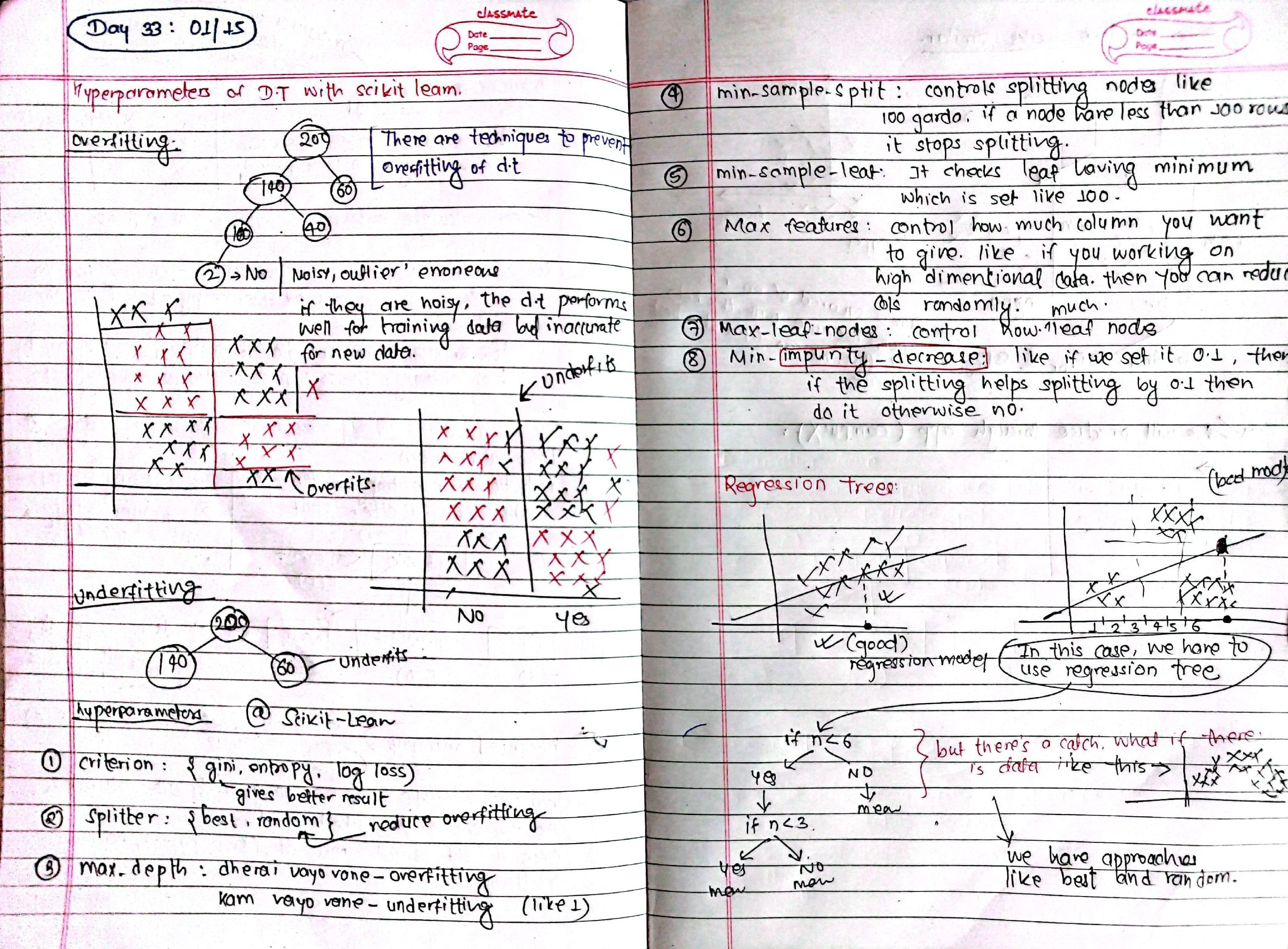
Studied hyperparameters of Decision Trees in Scikit-learn and techniques to handle overfitting and underfitting.
- Criterion (gini, entropy, log loss): Determines the quality of a split.
- Splitter: Helps reduce overfitting with better random splits.
- Max Depth: Controls tree depth; too high causes overfitting, too low causes underfitting.
- Min Sample Split: Sets the minimum samples required to split a node.
- Min Sample Leaf: Sets the minimum samples per leaf.
- Max Features: Determines how many features to use for splits.
- Max Leaf Nodes: Limits the number of leaf nodes.
- Min Impurity Decrease: Controls splitting based on impurity reduction.
A Regression Tree predicts continuous variables by splitting data to minimize variance. The best split is determined by maximizing variance reduction, calculated as the variance of the root node minus the weighted average variance of the leaf nodes.
Code:
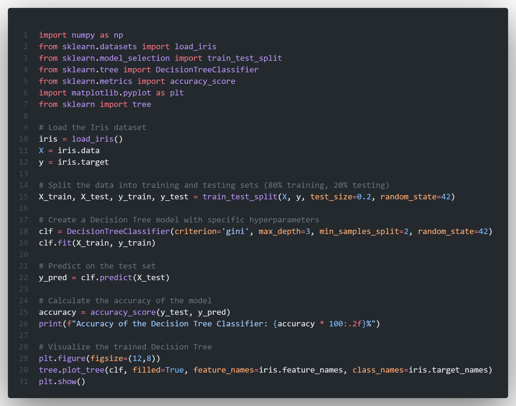 Output:
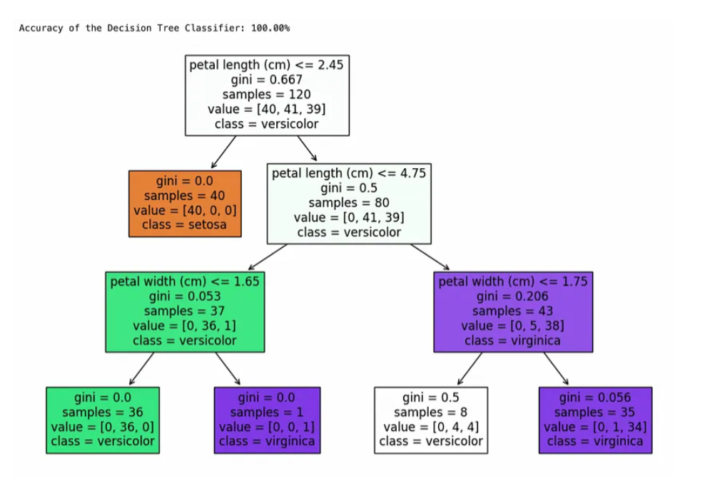
Day 34: Visualization Using dtreeviz, Ensemble Learning Overview
Notebook: Visualization of Decision Tree Official Notebook: Visualization of Decision Tree
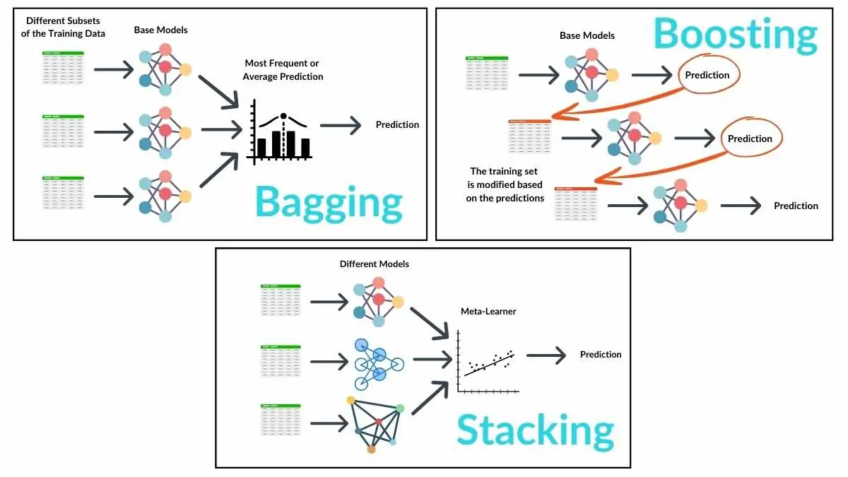
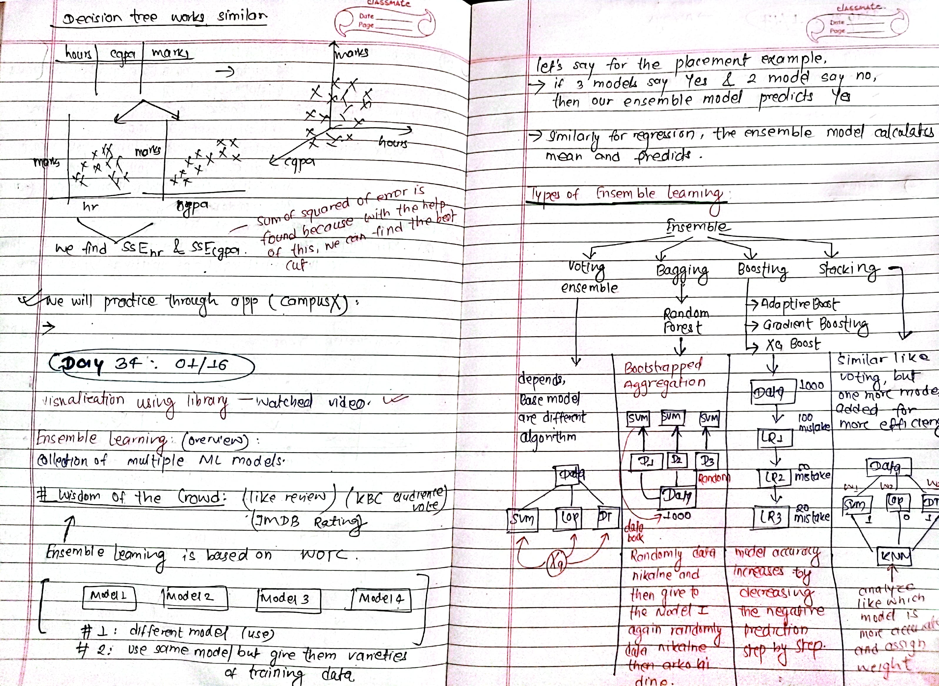
- started learning about ensemble learning: understood the concept of "wisdom of the crowd" in ensemble methods. types of ensemble methods: voting, bagging, boosting, and stacking. overview of random forest and bootstrapped aggregation (bagging). learned how boosting adjusts predictions iteratively.
Visuals of Bagging, boosting and stacking:
 Notes;
Day 35: Voting Ensemble > Classification and Regression
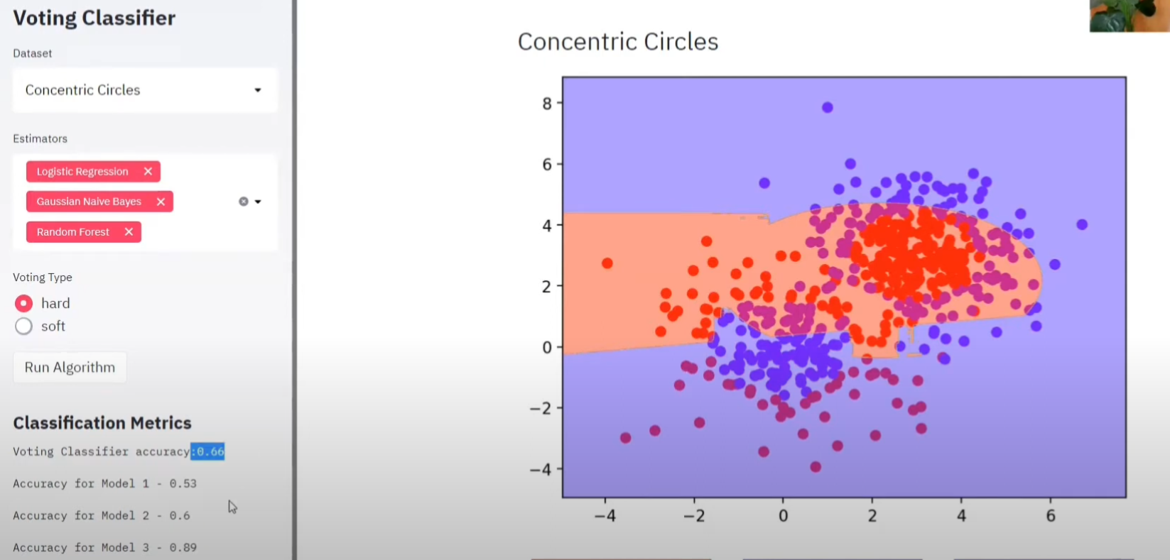
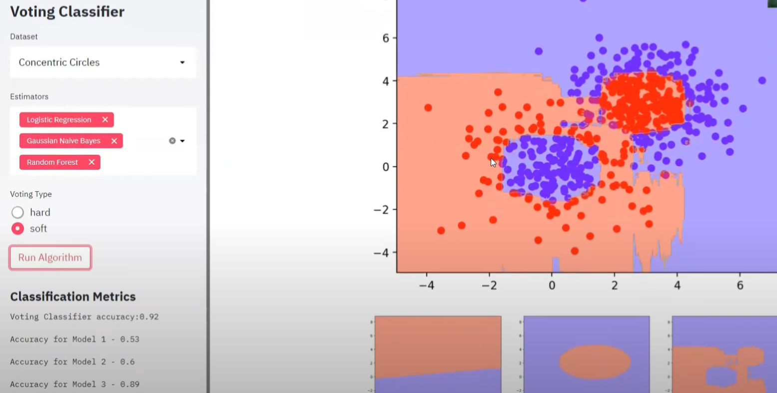
-
Soft voting: logistic regression: 60% fraud, random forest: 80% fraud, svm: 40% fraud → final probability: (60% + 80% + 40%) / 3 = 60%.
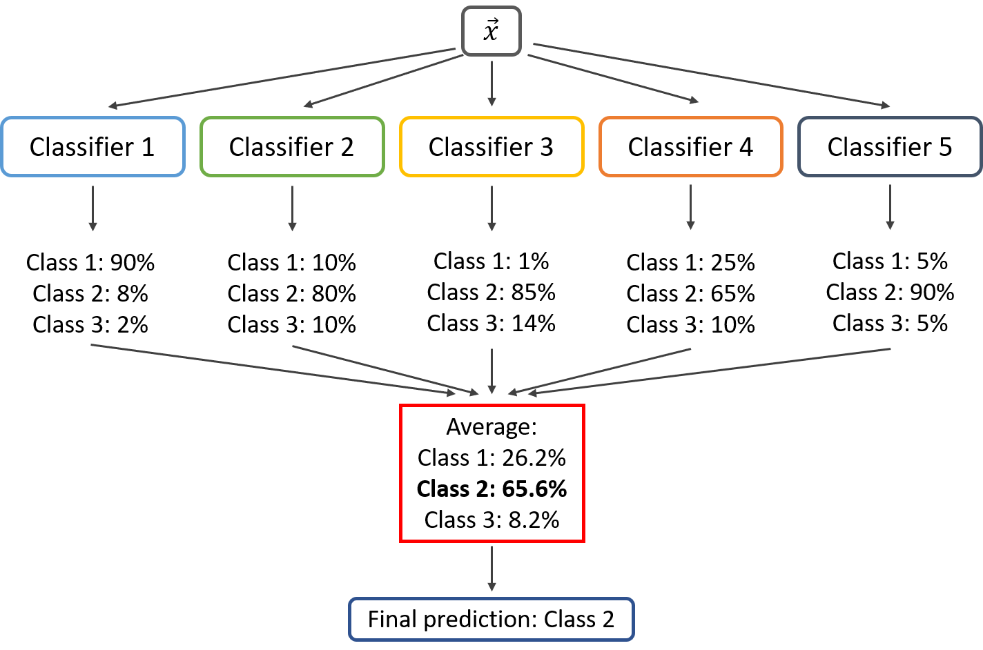
-
Hard voting: majority wins, logistic regression predicts "fraud," random forest predicts "not fraud," and svm predicts "fraud" → final prediction: "fraud."
Conclusions from Notebook: voting Classifier
-
weighted voting: assigning weights to classifiers helps emphasize stronger models, further improving performance.
-
same algorithm, different hyperparameters: tweaking hyperparameters (e.g., kernel degree in SVM) can lead to significant accuracy changes, highlighting the value of hyperparameter optimization.
Classification:
voting_clf = VotingClassifier(
    estimators=[
        ('lr', log_reg),  # logistic regression: good for linear patterns
        ('rf', rand_forest),  # random forest: captures complex relationships
        ('svc', svm_clf)  # support vector machine: handles edge cases
    ],
    voting='soft',  # averages probabilities from all models for final prediction
    weights=[2, 1, 1],  # gives higher importance to logistic regression
    n_jobs=-1  # enables parallel processing for faster training
)
What to use? soft voting or hard voting, depends if possible use both and then try to find out:
Regression:
- voting regressor combines multiple regression models to predict continuous values.
similarly, in regression, soft voting averages continuous predictions, and weighted voting helps models with higher performance contribute more.
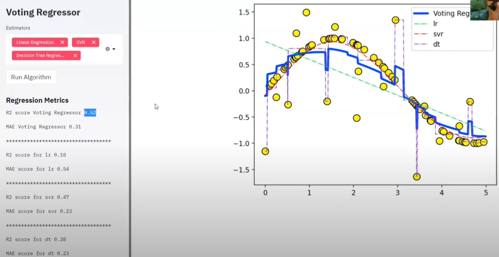
Visualize voting regression here: link
voting_reg = VotingRegressor(
    estimators=[
        ('lr', lin_reg),  # linear regression: good for linear relationships
        ('rf', rand_forest_reg),  # random forest regressor: handles non-linear patterns
        ('svr', svr_clf)  # support vector regressor: captures complex relationships
    ],
    weights=[2, 1, 1],  # assigns higher importance to linear regression
    n_jobs=-1  # enables parallel processing for faster training
)
Day 36: Bagging Ensemble > Classification and Regression
-
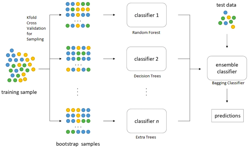
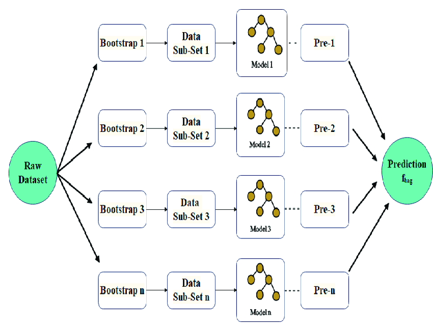
bagging (bootstrap aggregating) is an ensemble learning technique that combines predictions from multiple models trained on different subsets of the data (created via bootstrapping) to improve accuracy and reduce variance.
-
Intution:
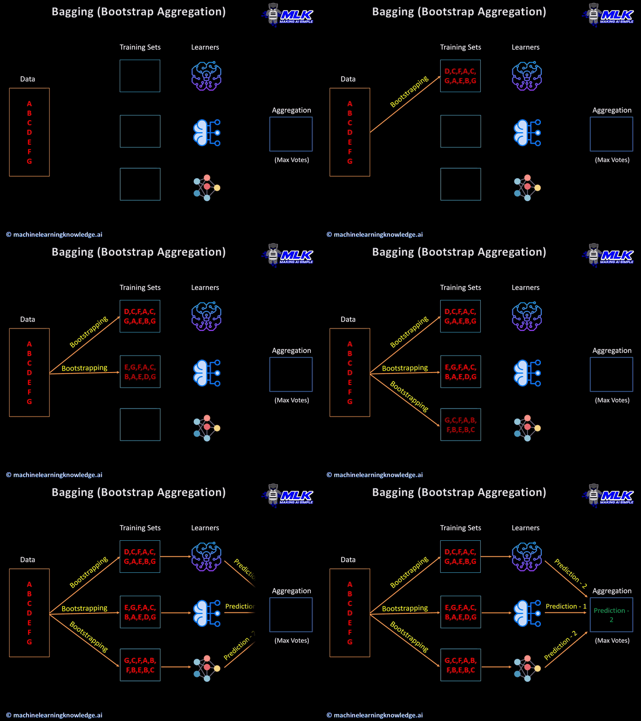
- random sampling: create multiple datasets by sampling with replacement from the original dataset.
- train independently: train a model (single preferred) on each bootstrapped dataset (e.g., decision trees).
- combine predictions: aggregate their predictions by majority voting (classification) or averaging (regression). this reduces overfitting and increases stability, especially for high-variance models.
Classification:
- Intution
- Code Demo
from sklearn.ensemble import BaggingClassifier
from sklearn.tree import DecisionTreeClassifier

# initialize the bagging classifier
bagging_model = BaggingClassifier(
    base_estimator=DecisionTreeClassifier(),  # base model for ensemble; here, decision trees
    n_estimators=10,                          # number of base models to train
    max_samples=1.0,                          # fraction of the dataset for each base model (1.0 = 100%)
    max_features=1.0,                         # fraction of features used in each bootstrap sample
    bootstrap=True,                           # sample datasets with replacement (True enables bootstrapping)
    bootstrap_features=False,                 # sample features with replacement (False = no feature bootstrapping)
    random_state=42                           # seed for reproducibility
)
Regression:
- Intution:
- Code Demo:
bagging_model = BaggingRegressor(
    base_estimator=DecisionTreeRegressor(),  # base model for ensemble; here, decision trees
    n_estimators=10,                          # number of base models to train
    max_samples=1.0,                          # fraction of the dataset for each base model (1.0 = 100%)
    max_features=1.0,                         # fraction of features used in each bootstrap sample
    bootstrap=True,                           # sample datasets with replacement (True enables bootstrapping)
    bootstrap_features=False,                 # sample features with replacement (False = no feature bootstrapping)
    random_state=42                           # seed for reproducibility
)
Day 37: Random Forest: Intution, Working and difference with bagging, Random Forest Hyperparameters
random forest is like a bunch of decision trees making a group decision. each tree gets a vote on the outcome, and the most votes win. it's like asking a bunch of experts for advice and going with the majority.
Sampling Techniques:
- row sampling
- column sampling
- combination
Random Forest vs bagging:
-
why random forest performs well: it reduces overfitting by averaging multiple decision trees trained on different random subsets of data and features, improving accuracy and robustness.
-
random forest vs bagging: both use multiple trees, but random forest adds feature randomness at each split, making trees less correlated and boosting performance.
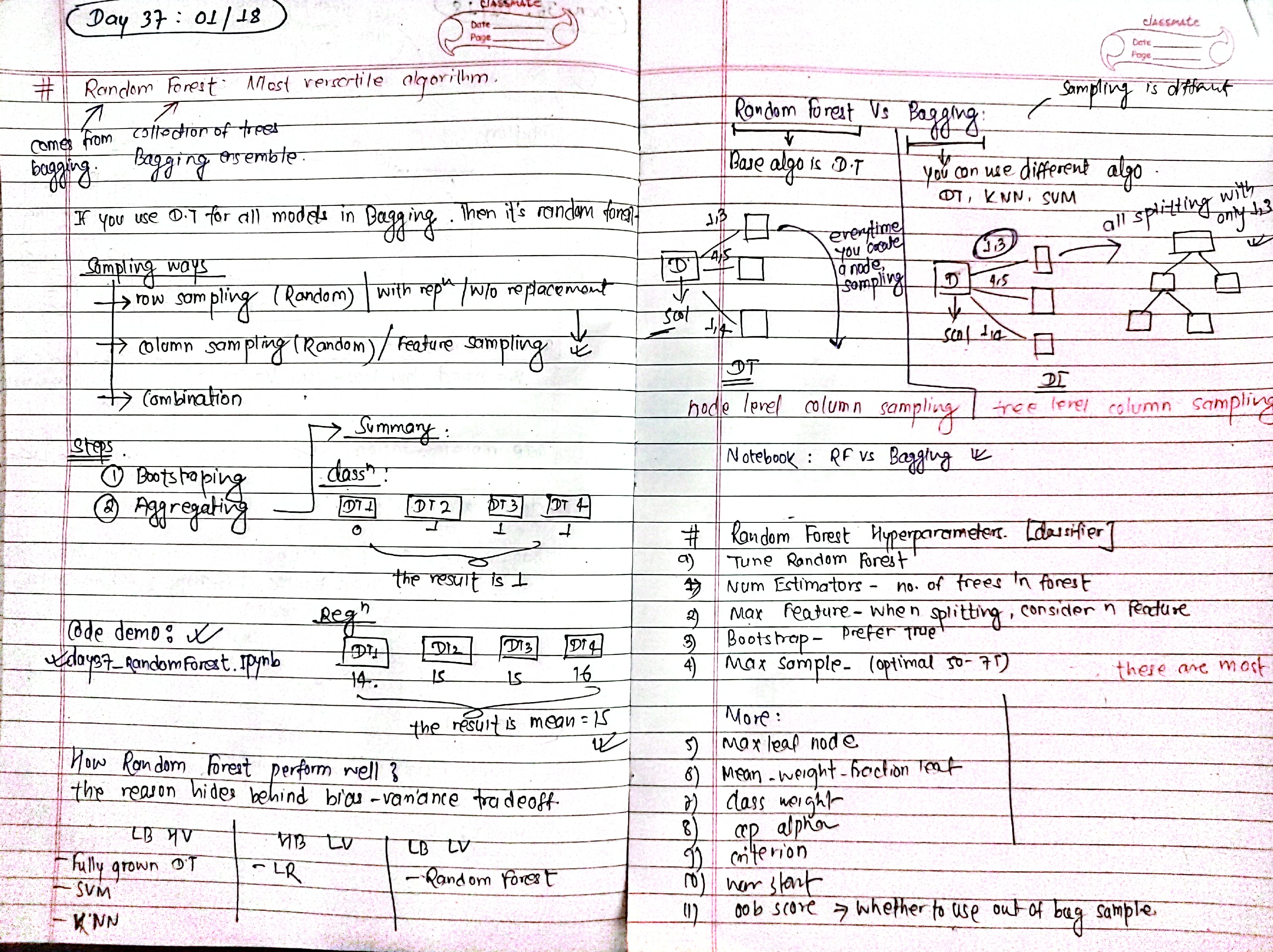
Notebook: Random forest Vs bagging
Random forest Hyperparameters:
model = RandomForestClassifier(
    # core hyperparameters
    n_estimators=100,         # number of decision trees in the forest
    max_features="sqrt",      # max features to consider at each split
    max_depth=None,           # max depth of each tree; None = grow fully
    min_samples_split=2,      # min samples needed to split a node
    min_samples_leaf=1,       # min samples required in a leaf node
    bootstrap=True,           # with replacement or without replacement

    # advanced hyperparameters
    max_leaf_nodes=None,      # max number of leaf nodes per tree; None = unlimited
    min_weight_fraction_leaf=0.0,  # min fraction of total weight for a leaf node
    class_weight=None,        # weights for handling class imbalance (e.g., 'balanced')
    ccp_alpha=0.0,            # complexity parameter for pruning; trade-off between size and accuracy
    criterion="gini",         # metric to evaluate splits: "gini" (default) or "entropy"
    warm_start=False,         # reuse previous trees for incremental training; False = train from scratch
    oob_score=False,          # whether to use out-of-bag samples to estimate generalization accuracy
    verbose=0,                # verbosity of output (0 = silent)
    n_jobs=-1,                # number of CPU cores for parallel processing; -1 = use all cores
    random_state=42           # seed for reproducibility
)
Day 38: Boosting Ensemble: Adaboost Boosting
- boosting is a sequential ensemble learning method where models correct the errors of previous models to reduce bias.
combines weak learners (like decision stumps) to create a strong predictive model.
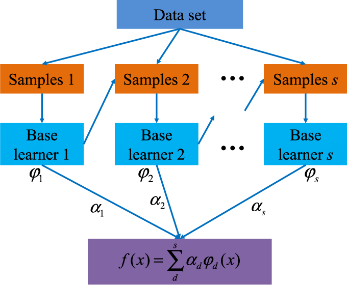
Notes:
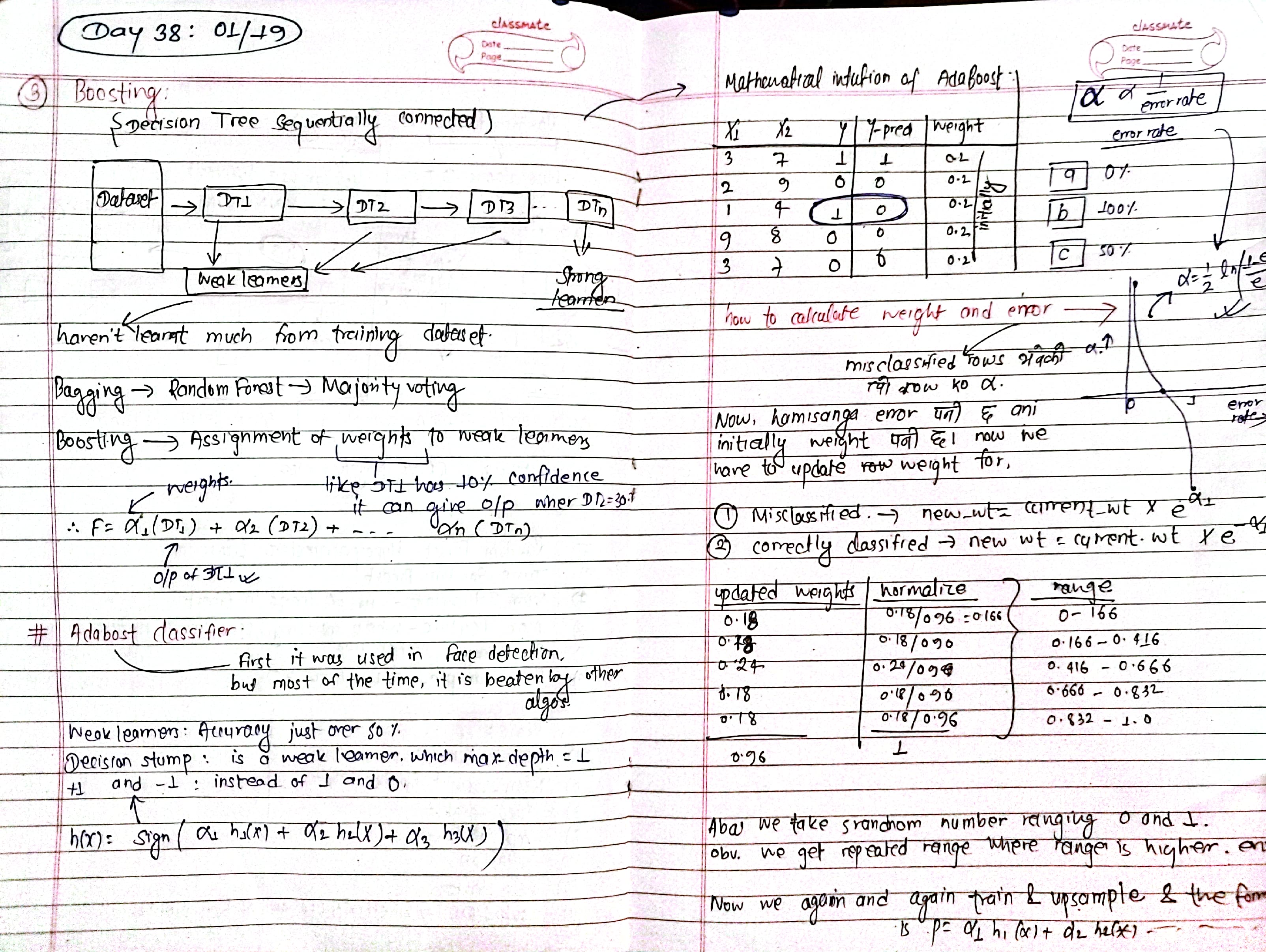
AdaBoost Exploration:
step-by-step understanding of adaboost’s workflow, including:
- calculating sample weights and weak learner errors.
- updating model contributions based on performance.
- final prediction via weighted majority vote.
- visualized how adaboost focuses on difficult samples.
implemented adaboost from scratch without using sklearn.
Notebook: Adaboost Implementation
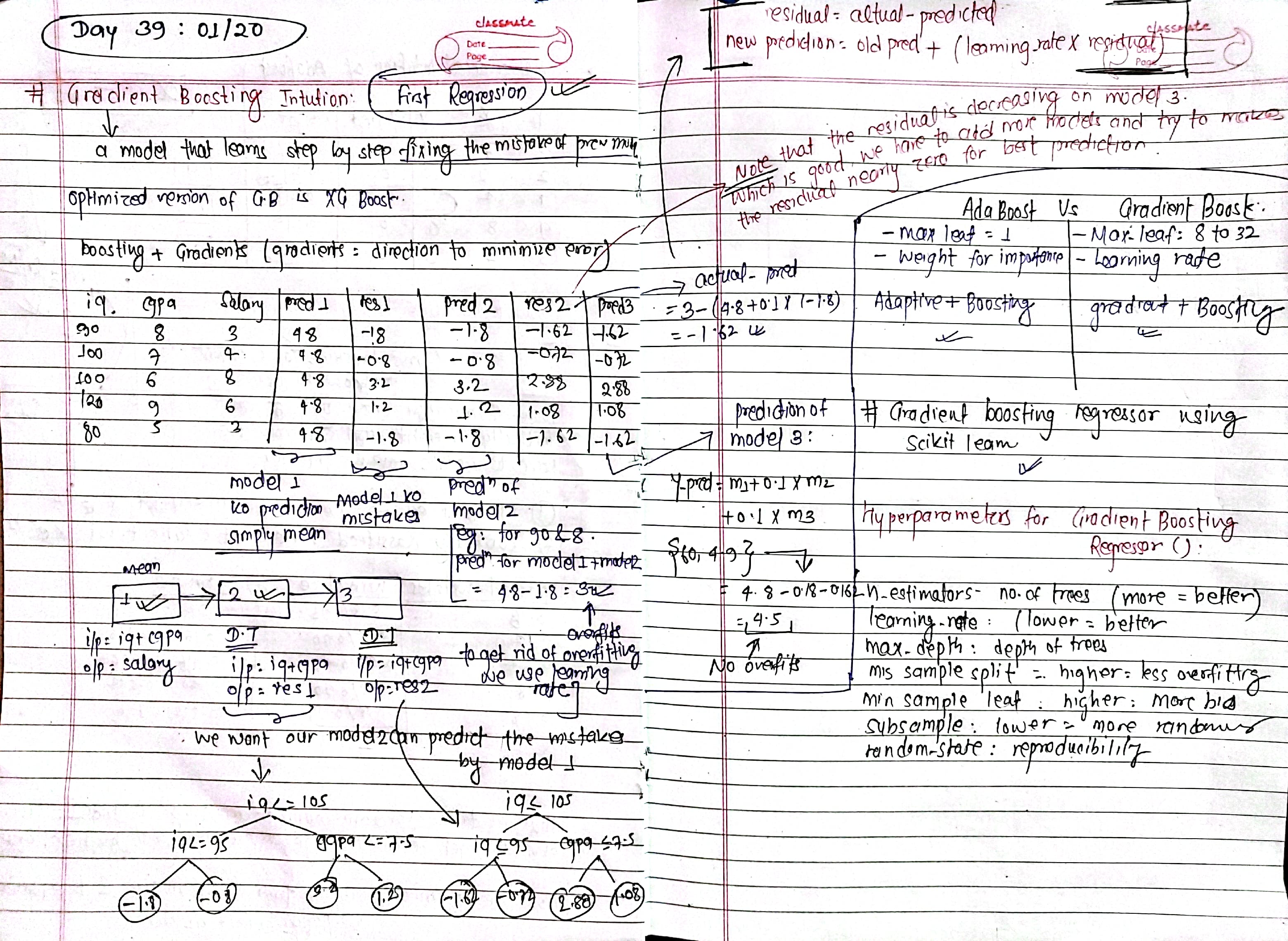
Day 39: Understanding GradientBoosting with Regression:
"a model that learns step-by-step by fixing the mistakes of the previous model."
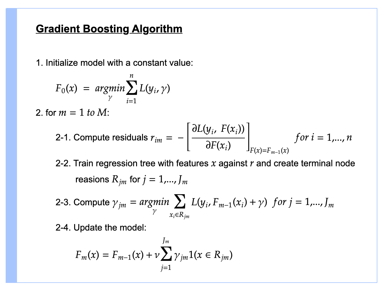
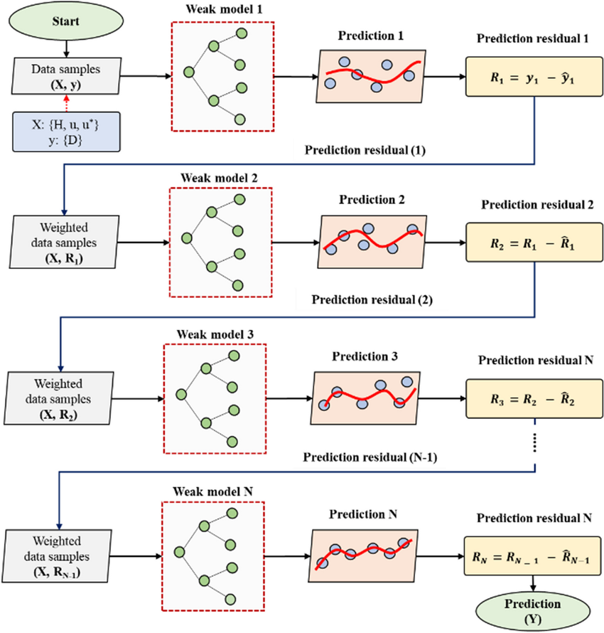
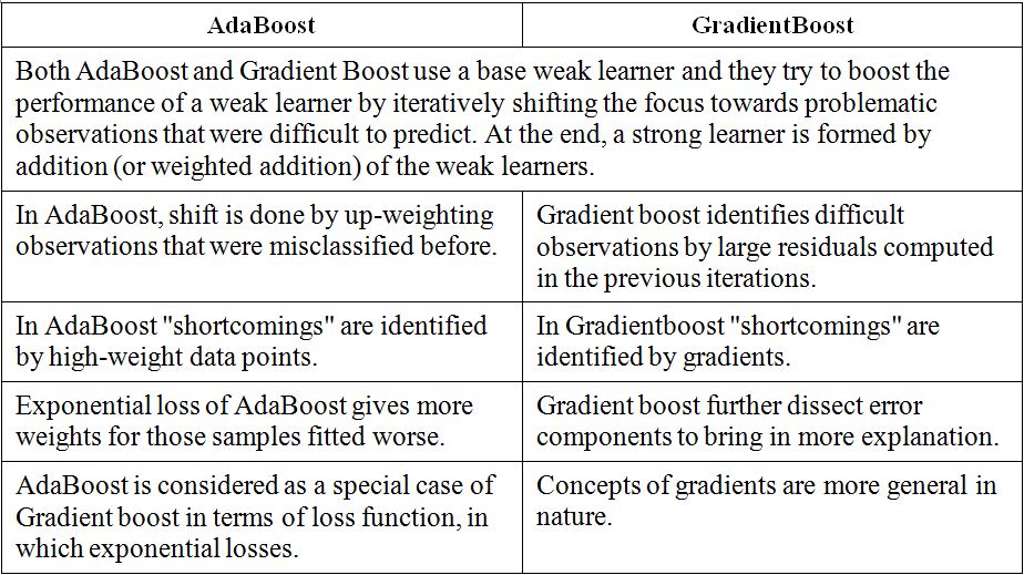
- Comparision between Adaboost and Gradietn boost:
boosting + gradients (gradients = direction to minimize error).
pseudo-  residual = actual - predicted
new prediction = old prediction + (learning_rate × residual)
gradient boosting variations:
- xgboost: uses regularization and handles missing data efficiently.
- lightgbm: faster with large datasets.
- catboost: great for categorical data.
    gb = GradientBoostingRegressor(
        n_estimators=100,      # number of trees
        learning_rate=0.1,     # step size for updates
        max_depth=3,           # depth of each tree
        min_samples_split=2,   # min samples to split a node
        min_samples_leaf=1,    # min samples per leaf
        subsample=1.0,         # fraction of samples per tree
        max_features=None,     # use all features
        random_state=42        # ensures reproducibility
    )
Notes:
Day 40: Gradient Boosting with Classification
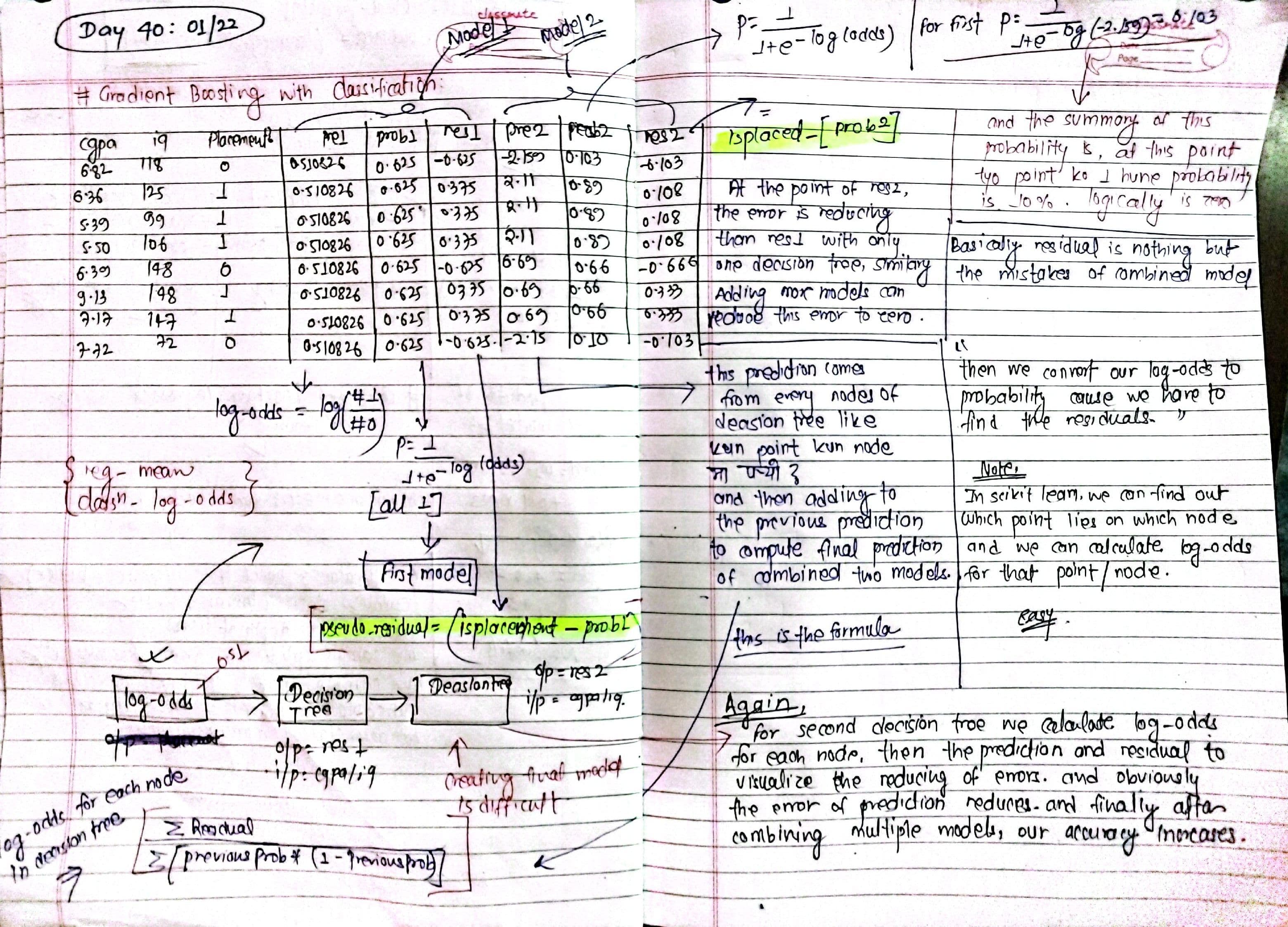
Overview
- Gradient boosting improves classification by minimizing log-loss iteratively.
- Each tree focuses on correcting errors made by previous trees.
- Uses gradients of the loss function to guide updates.
Algorithm
- Initialize predictions:
F0(x)(log-odds for classification). - For each iteration:
- Compute pseudo-residuals:
ri = - ∂(loss) / ∂F(xi) - Fit a weak learner (tree) to
ri. - Update predictions:
F(x) = F(x) + η * h(x)
whereηis the learning rate.
- Compute pseudo-residuals:
Loss Function
- Binary classification: log-loss.
Loss = -[y log(p) + (1 - y) log(1 - p)] - Multiclass classification: softmax loss.
gb = GradientBoostingClassifier(
    n_estimators=100,
    learning_rate=0.1,
    max_depth=3,
    random_state=42
)
Notes:
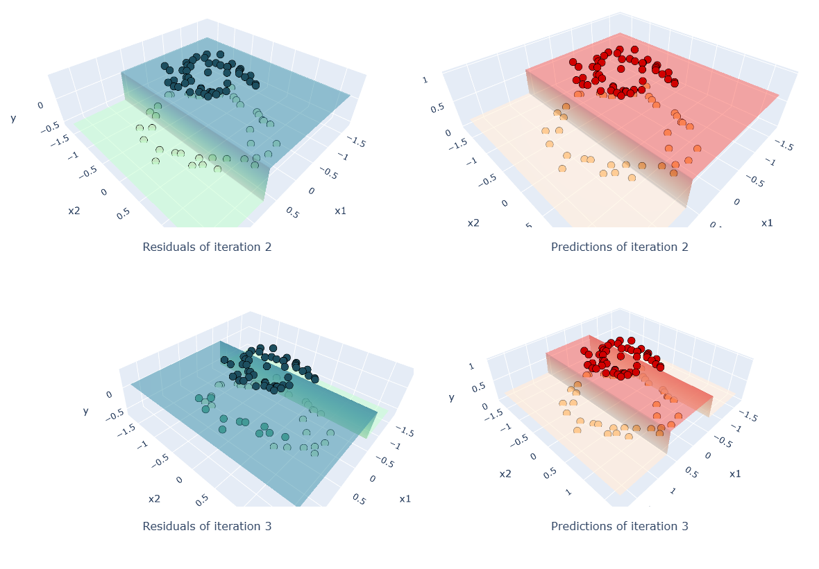
Notebook: Gradient Boosting Classification
Visuals:
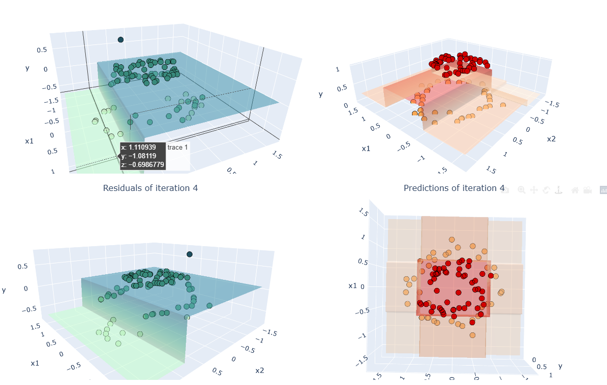
Day 41: Variations of Gradient Boosting: XGBoost - Introduction.
- xgboost
- lightgbm
- catboost
XGBoost:
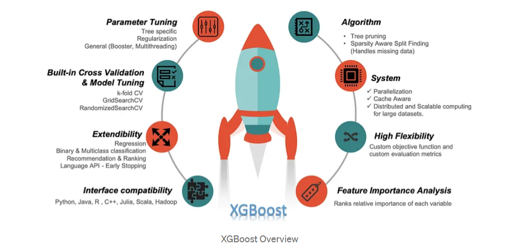 xgboost (eXtreme Gradient Boosting) is an advanced implementation of gradient boosting that addresses some key limitations in traditional gradient boosting and adaboost.
here's a quick rundown of what i've learned so far.
xgboost (eXtreme Gradient Boosting) is an advanced implementation of gradient boosting that addresses some key limitations in traditional gradient boosting and adaboost.
here's a quick rundown of what i've learned so far.
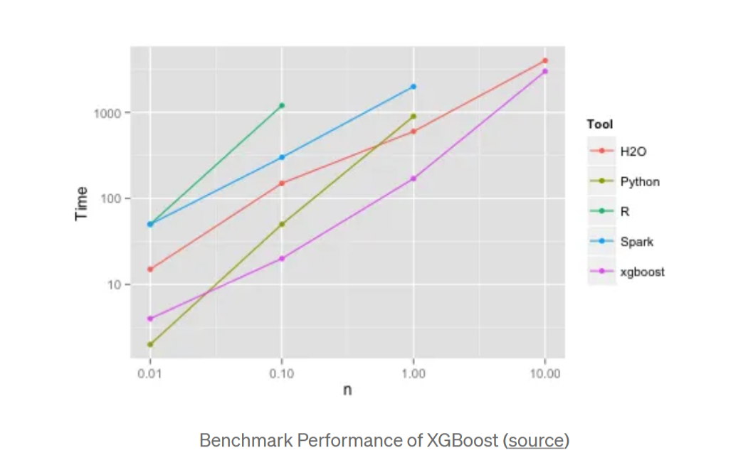
-
Flexibility
- cross-platform support means xgboost works on different operating systems without much hassle.
- it supports multiple languages like python, c++, and r, which makes it easy to integrate with your preferred tech stack.
- integrating with other libraries like scikit-learn or spark is a breeze.
- it can handle all kinds of ml problems — whether it's classification, regression, or ranking.
-
Speed
- parallel processing is key. it uses all your cores to speed things up, so you get faster results.
- optimized data structures (like DMatrix) help reduce memory usage and make computations more efficient.
- it’s cache-aware, so it knows how to make use of your cpu cache and speed up data retrieval.
- xgboost handles datasets larger than memory through out-of-core computing.
- distributed computing helps when your dataset is huge and you need to scale your work across multiple machines.
- with gpu support, xgboost accelerates matrix calculations, making it much faster for large datasets.
-
Performance (Why this is different from other algos??)
- regularization is a big win. it prevents overfitting with L1 and L2 regularization, keeping your model generalizable.
- it automatically handles missing values, learning the best way to fill them in.
- sparsity-aware split finding is great for sparse data (think text data or categorical features).
- finding efficient splits in trees is another xgboost feature that speeds up training without compromising accuracy.
- tree pruning helps reduce tree size after training, improving the model’s performance on unseen data.
Day 42: XGBoost for Regression and Classification, Catboost Vs XGboost Vs LightGBM
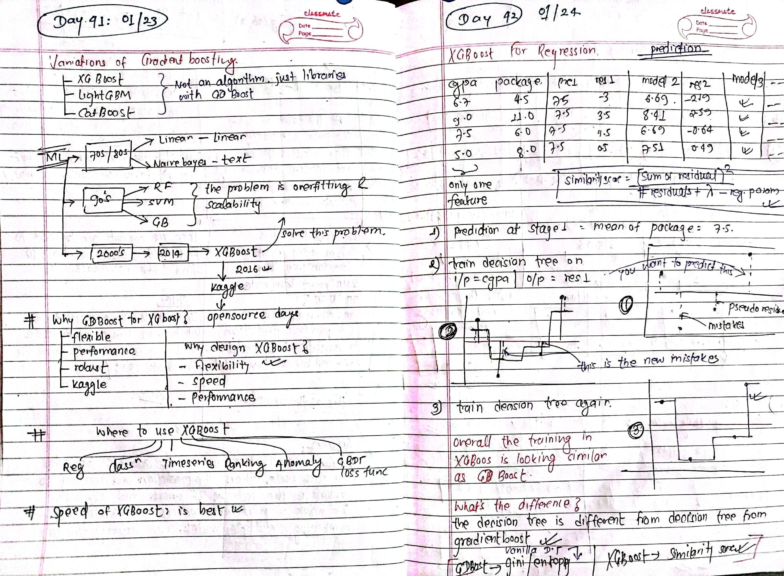
Notes on what i explored:
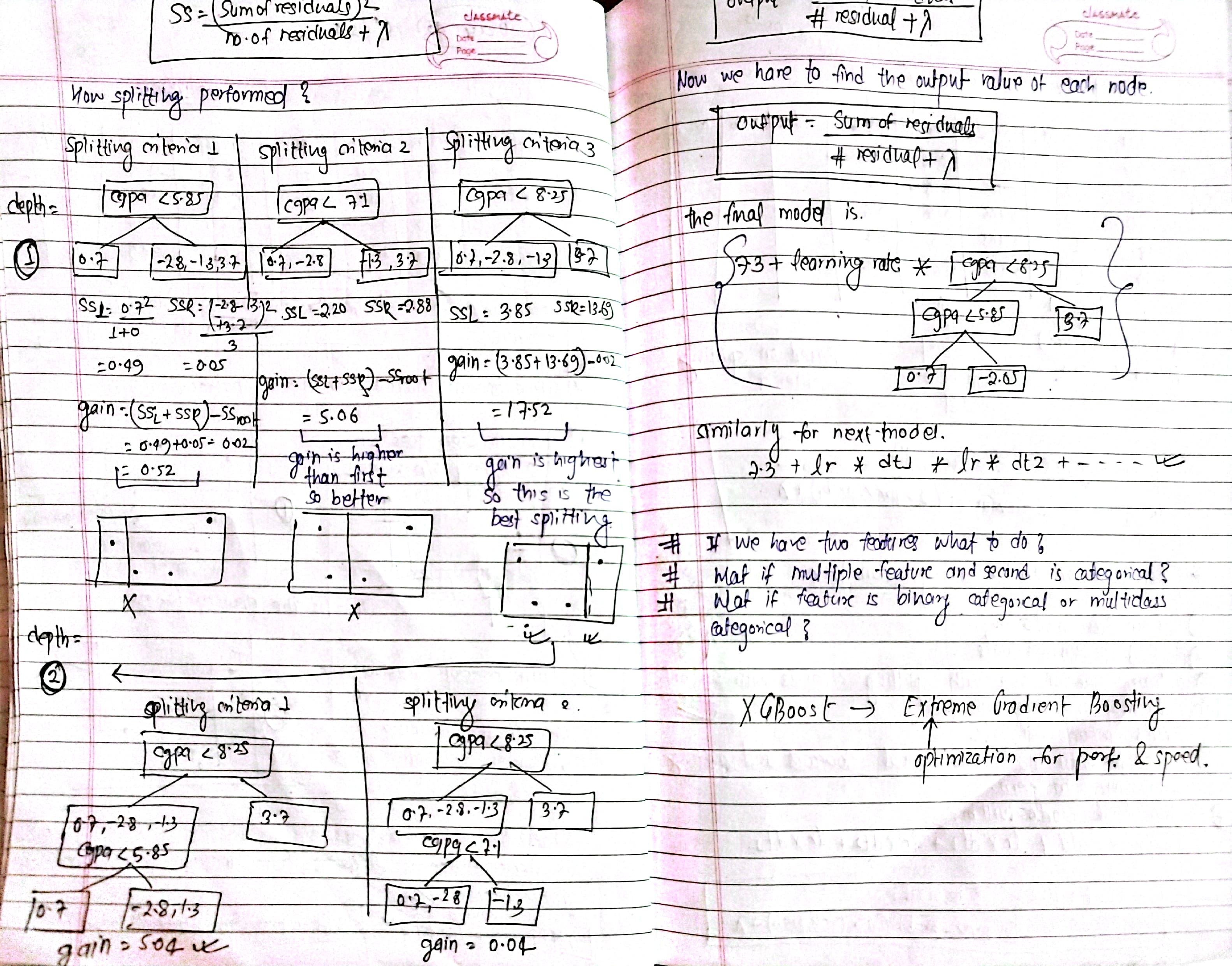
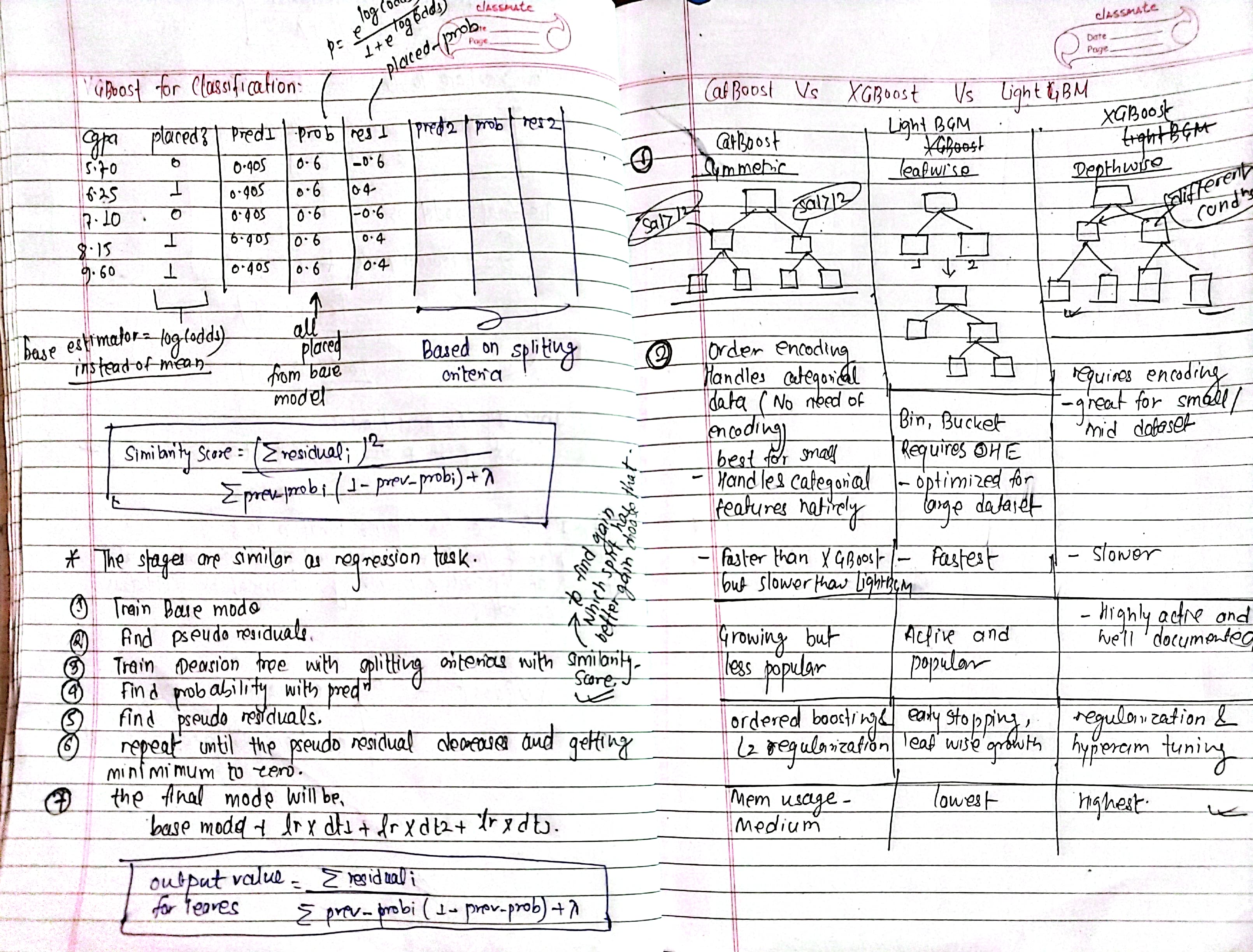
-
What if we have two or more than two features? We can scan all features , and do all possible splits for all features, then we will calculate gain and similarity score , and select feature which has max gain, algo use greedy search
-
What if multiple feature and second feature is categorical (like binary: yes/no, male/female or muticlass: colors)? You have to encode them using OHE or other. or use othre variants of GDboost. idenntify unique values in catagorical columns , and consider both as a potential split point ., then calculate gain and similarity scores ., and select with maximum gain .
-
What if the feature is binary categorical or multiclass categorical? older versions: encode them (e.g., one-hot, label, or target encoding). newer versions: native support for categorical features—no encoding needed.
Catboost Vs LightGBM Vs XGBoost:
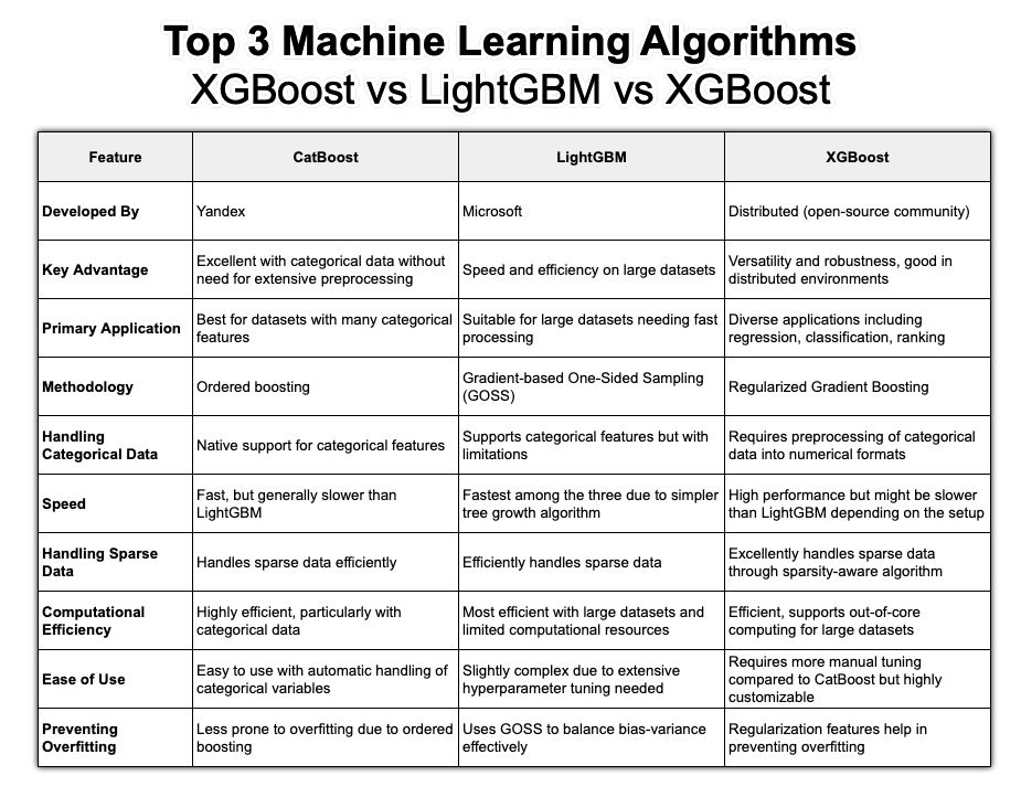
- categorical features
- catboost handles them natively—no encoding needed.
- lightgbm/xgboost require encoding, but xgboost supports label encoding in newer versions.
- speed
- lightgbm is the fastest, especially for large datasets.
- catboost is slower but optimized for small/mid datasets.
- xgboost is slower than both due to its exhaustive computations.
- memory usage
- lightgbm uses the least memory.
- catboost and xgboost consume more, especially xgboost for large datasets.
- overfitting prevention
- all three handle overfitting well, but catboost excels in datasets prone to overfitting due to ordered boosting.
- use case
- catboost: small/mid datasets with many categorical features.
- lightgbm: large datasets where speed and memory are critical.
- xgboost: general-purpose, robust across various dataset types.
Day 43: Stacking Ensemble: Understanding Blending and K-fold methods
~ blending: splits the data into a training set and a holdout set to train base models and then a meta-model on the predictions of the base models.~
~ k-fold stacking: uses cross-validation to generate predictions for the meta-model by training base models on different training folds and predicting on the validation fold. ~
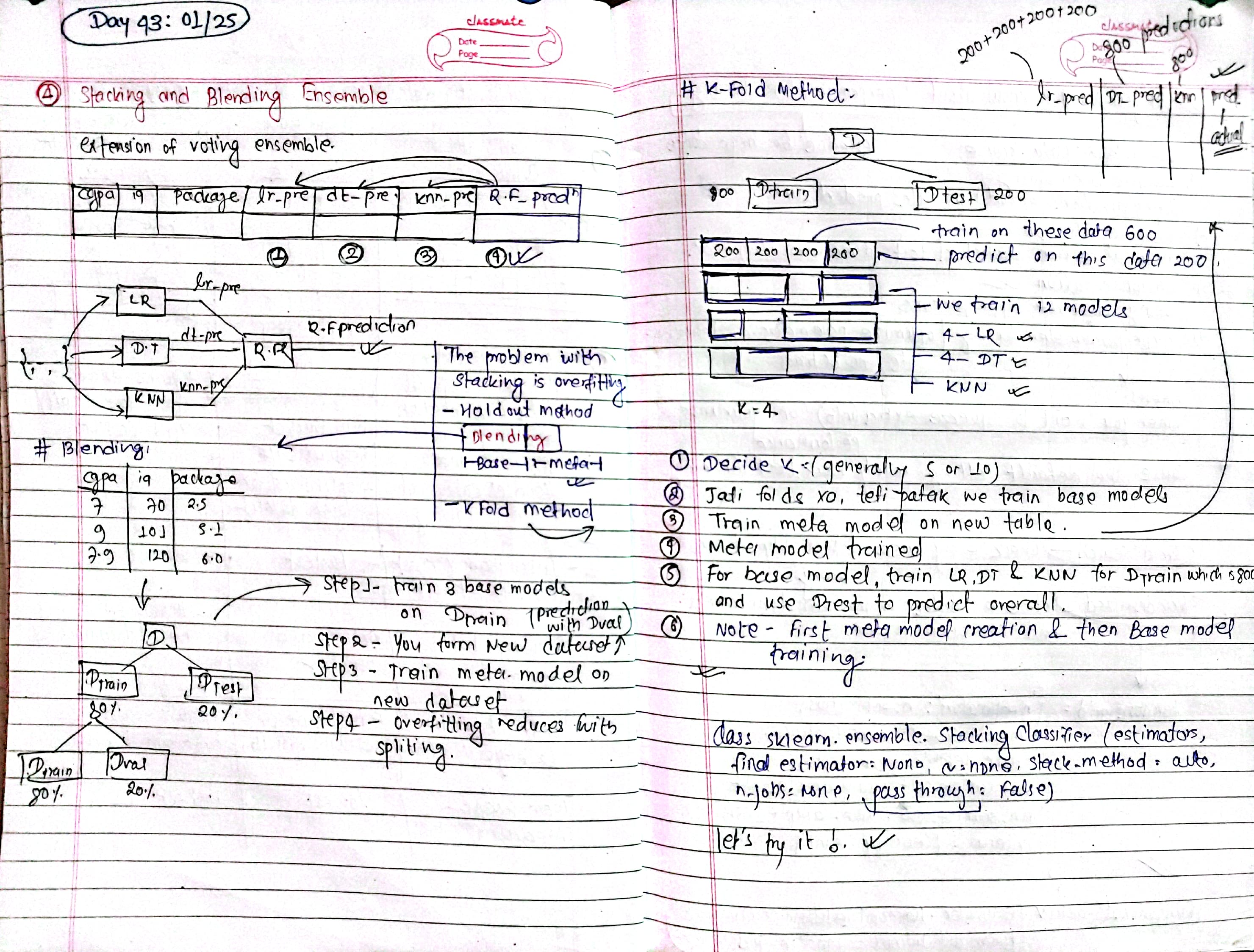
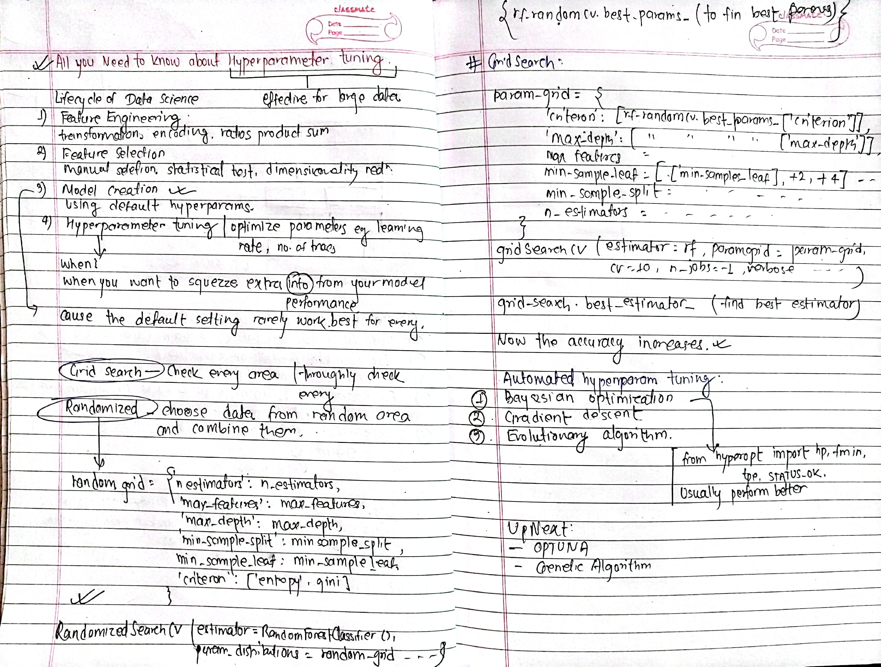
!Hyperparameters Tuning:
- identify hyperparameters: for decision trees: max_depth, min_samples_split, etc. for neural networks: learning rate, batch size, number of layers, etc.
- choose a tuning method: grid search: try every combination of parameters (computationally expensive). random search: test random combinations (faster). bayesian optimization: automatically find the best parameters using probabilistic methods. automated tuning: libraries like optuna or hyperopt.
- cross-validate: use k-fold cross-validation to test parameter combinations.
- pick the best:
finalize hyperparameters that minimize error metrics or maximize accuracy.
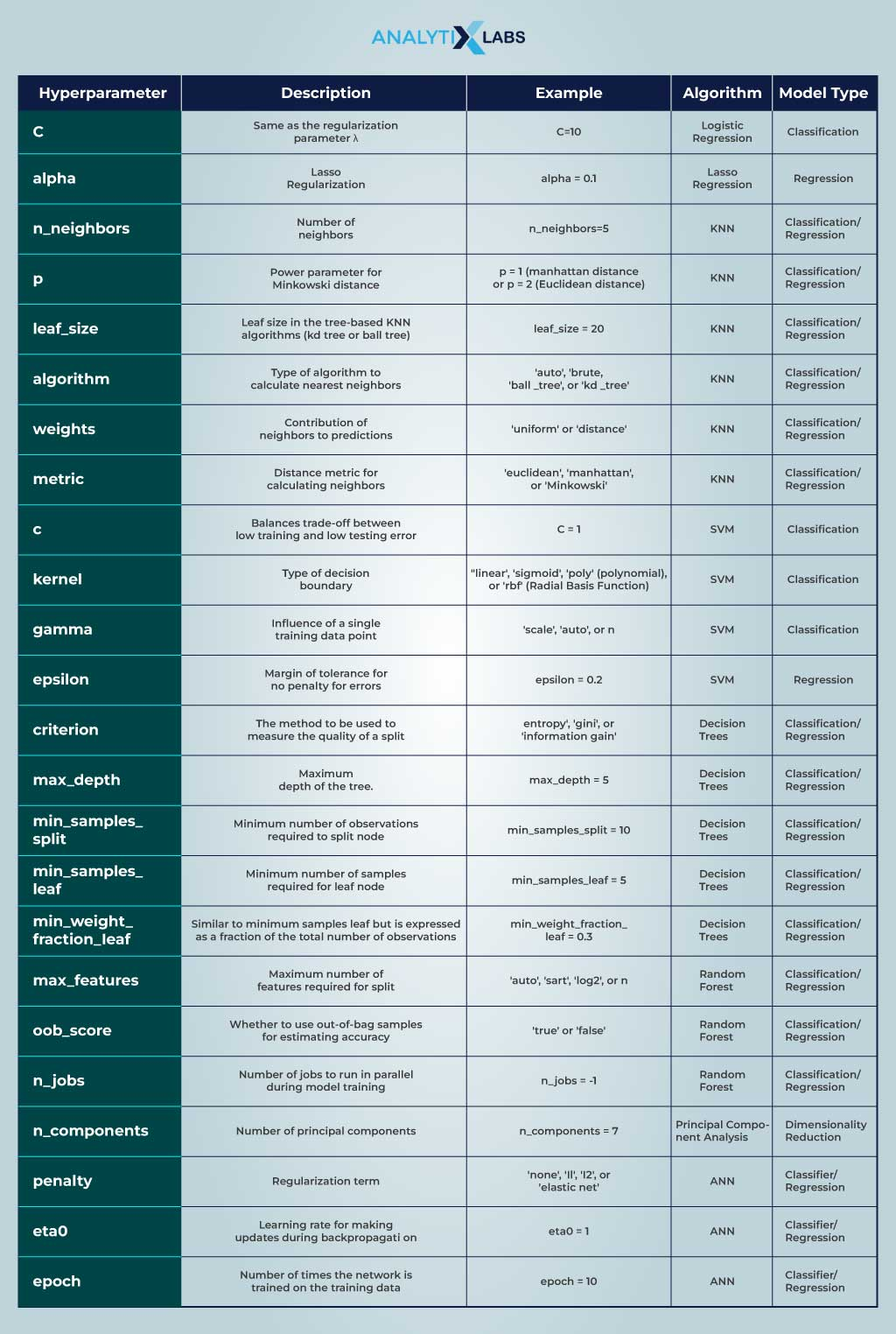
1. manual tuning
- tweak hyperparameters based on experience or trial-and-error.
- works for simple models but not scalable.
2. grid search
-
systematically tests all combinations of hyperparameter values.
-
pros: exhaustive, finds the best combo (if time permits).
-
cons: computationally expensive, impractical for large spaces.
-
example:
from sklearn.model_selection import GridSearchCV
param_grid = {'max_depth': [3, 5, 10], 'min_samples_split': [2, 5, 10]}
grid_search = GridSearchCV(DecisionTreeClassifier(), param_grid, cv=5)
grid_search.fit(X_train, y_train)
print(grid_search.best_params_)
3. random search
-
samples random combinations of hyperparameters.
-
pros: faster, effective for large search spaces.
-
cons: might miss optimal combinations.
-
example:
from sklearn.model_selection import RandomizedSearchCV
from scipy.stats import randint
param_dist = {'max_depth': randint(3, 20), 'min_samples_split': randint(2, 20)}
random_search = RandomizedSearchCV(DecisionTreeClassifier(), param_dist, n_iter=100, cv=5)
random_search.fit(X_train, y_train)
print(random_search.best_params_)
4. bayesian optimization
- predicts the best hyperparameters using probabilistic models (e.g., Gaussian processes).
- pros: efficient in high-dimensional spaces.
- cons: complex implementation.
- libraries:
Optuna,Hyperopt,BayesSearchCV.
5. evolutionary algorithms
- optimizes hyperparameters using natural selection (e.g., genetic algorithms).
- library:
TPOT.
6. automated tools
auto-sklearn: automates model selection + hyperparameter tuning.H2O.ai: distributed hyperparameter tuning.Optuna: fast, user-friendly library for hyperparameter search.
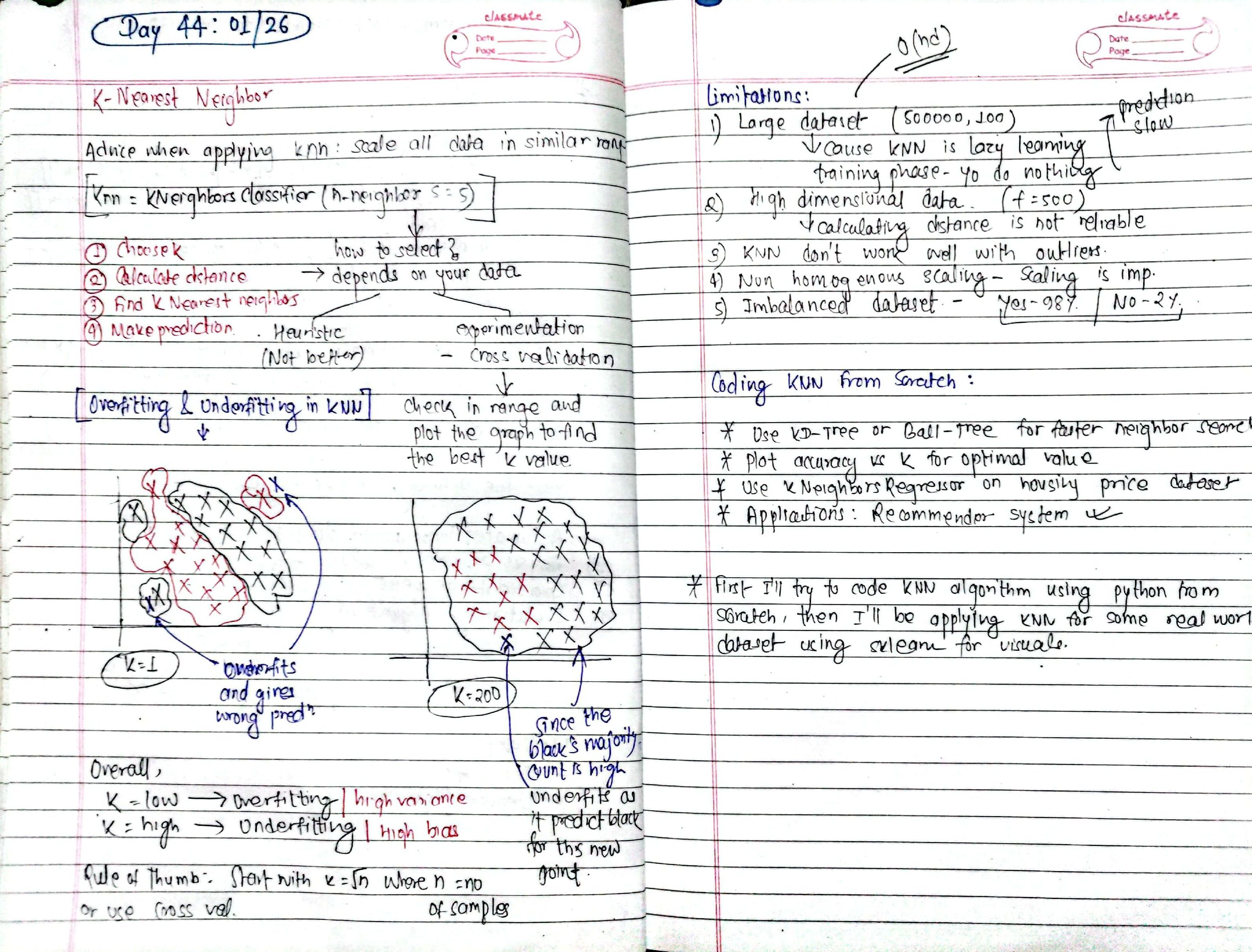
Day 44: K Nearest Neighbor, Coding KNN from scratch and applying on different datasets:
Predictions are based on the majority vote (classification) or average (regression) of the K closest data points in the training set.
Step-by-Step Workflow:
- Choose K: Number of neighbors to consider.
- Calculate Distance:
- Common metrics: Euclidean (default), Manhattan, or Minkowski.
- Find K Nearest Neighbors: Identify the K points closest to the query.
- Make Prediction:
- Classification: Majority class among neighbors.
- Regression: Average value of neighbors.
3. Choosing the Right K
- Small K (e.g., K=1): High variance, sensitive to noise (overfitting).
- Large K (e.g., K=50): High bias, smoother boundaries (underfitting).
- Rule of Thumb: Start with K=nK=n (where nn = number of samples) or use cross-validation.
Overfitting and Underfitting:
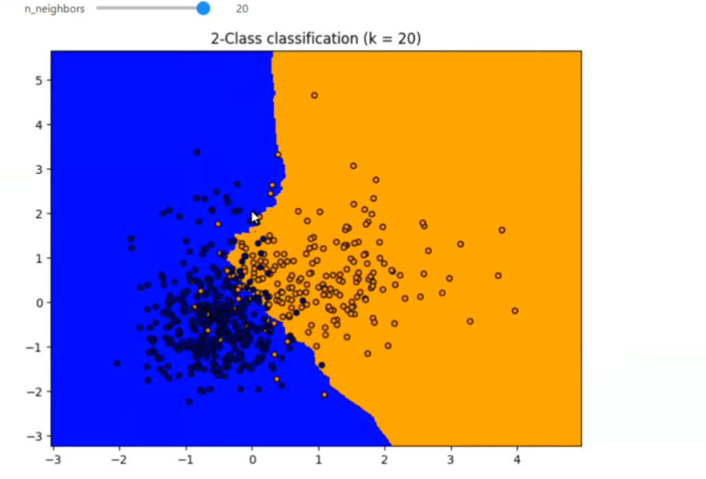
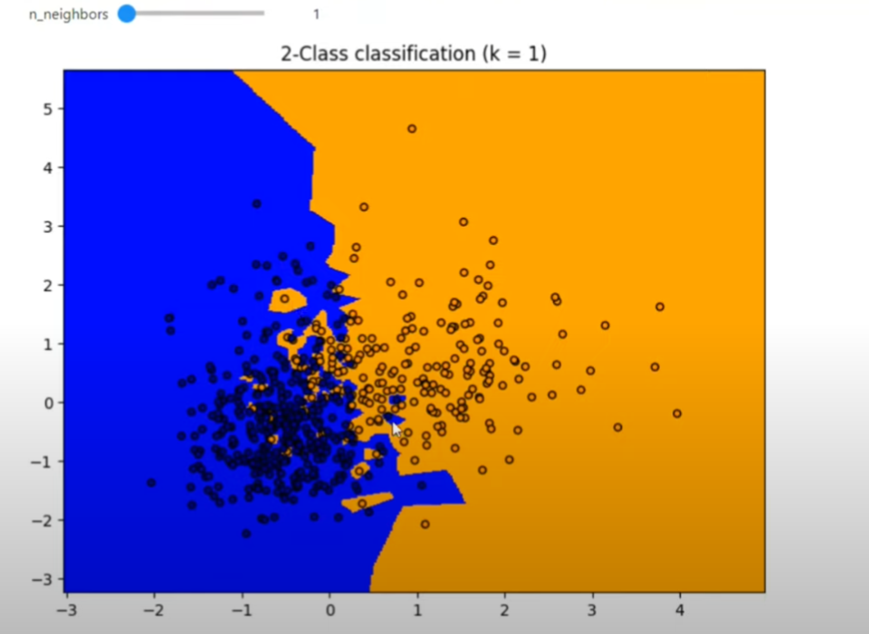
Code of KNN using Python:
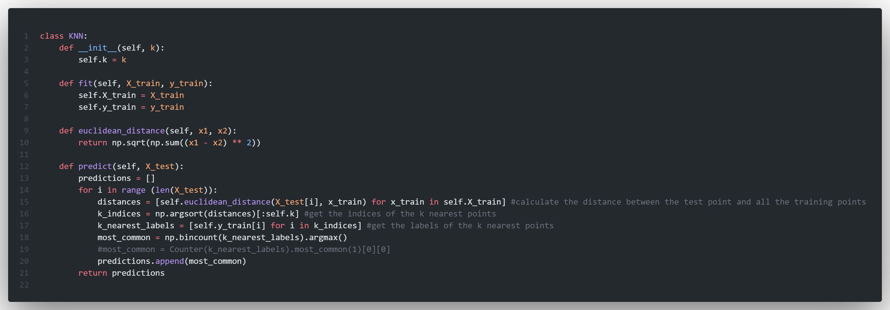
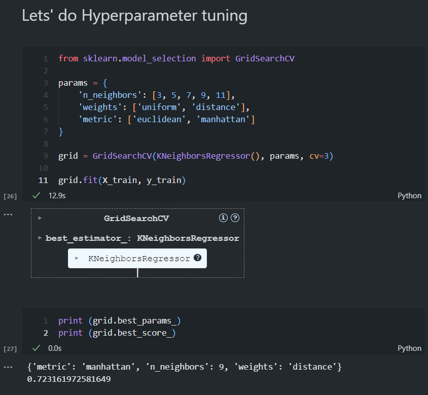
Finally After Hyperparameter tuning, KNN models imporves for California House price prediction:
Notes:
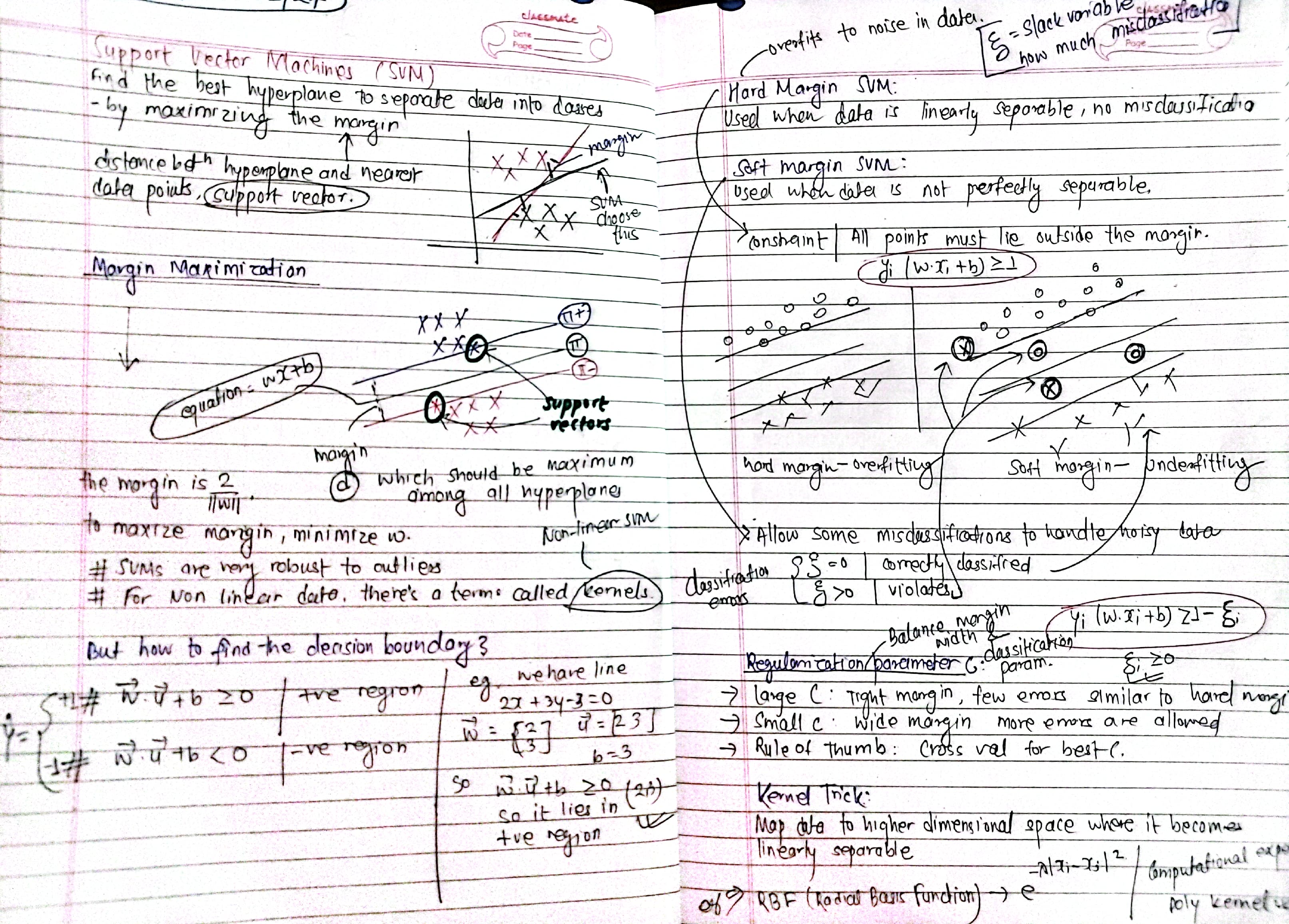
Day 45: Support Vector Machines:
- What is SVM? Goal: SVM finds the "best" hyperplane to separate data into classes.
Key Idea: Maximize the margin (distance between the hyperplane and the nearest data points, called support vectors).
- svm helps classify data by finding the best dividing line (hyperplane).
- support vectors: closest points to the line that influence its position. kind of like the apples and oranges closest to the ruler.
- margin: the gap between the line and the nearest points. svm tries to make this as wide as possible for better separation.
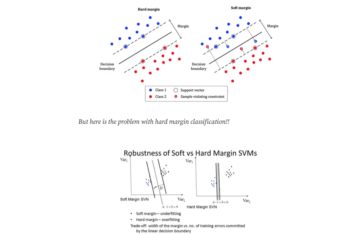
- hard margin svm: works only when data is clean and separable. not great for noisy or messy data.
- example: classifying perfectly labeled "cat" vs. "dog" images where there’s no overlap.
- soft margin svm: allows some mistakes for better flexibility with noisy/overlapping data.
- example: separating spam and non-spam emails, where some emails are hard to classify.
- kernel trick: useful when the data isn’t linearly separable. it projects data into a higher dimension to make it separable.
- example: in handwriting recognition, svm can map curvy letters into a higher space to separate them more easily.
More Notes like optimization regularization:
Day 46: K-Means Clustering, DBSCAN
K-Means (centeroid based):
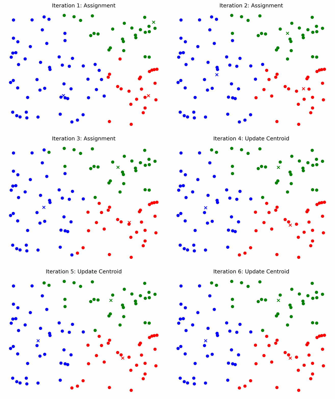
Algorithm Steps
- Initialize Centroids: Randomly select K data points as initial centroids(Can lead to suboptimal clusters.) (or use k-means++(Distributes initial centroids to improve stability and speed) for smarter initialization).
- Assign Points to Clusters: For each data point, compute the Euclidean distance- used by default to all centroids. Assign the point to the nearest centroid.
- Recalculate Centroids: Compute the mean of all points in each cluster to update centroids.
- Repeat: Reassign points and update centroids until:
- Centroids stabilize (change < tolerance threshold).
- Maximum iterations are reached.
Applications
- Customer Segmentation
- Image Compression
- Document Clustering
from sklearn.cluster import KMeans
from sklearn.preprocessing import StandardScaler

# Preprocess data
scaler = StandardScaler()
X_scaled = scaler.fit_transform(X)

# Fit K-means
kmeans = KMeans(n_clusters=3, init='k-means++', n_init=10)
kmeans.fit(X_scaled)

# Get labels and centroids
labels = kmeans.labels_
centroids = scaler.inverse_transform(kmeans.cluster_centers_)
Choosing the Optimal K
- Elbow Method: Plot inertia vs. K; the "elbow" (point where inertia decline slows) suggests optimal K.
- Silhouette Score: Measures how similar a point is to its cluster vs others. Higher score (closer to 1) = better clustering.
- Domain Knowledge: Use prior understanding of the data to guide K selection (e.g., customer segments in marketing).
Notebook: K-Means clustering Demo
One limitation of K-means is that you must specify the number of clusters beforehand.
DBSCAN (density based clustering)
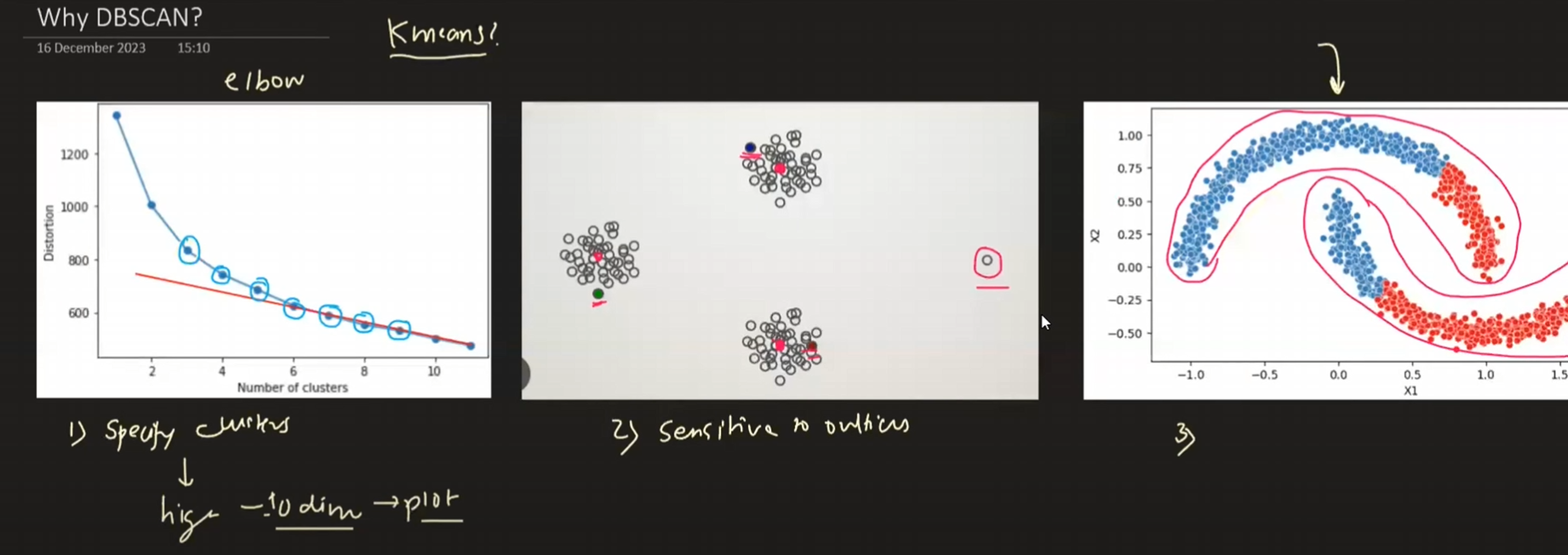
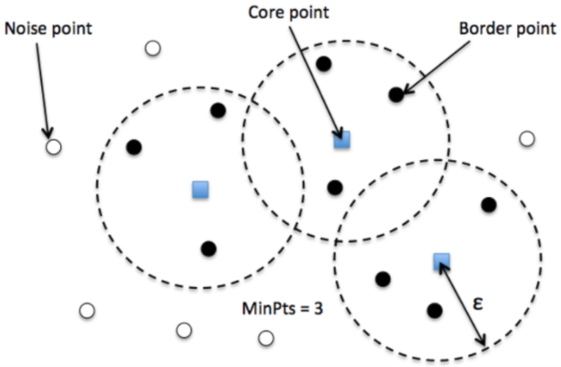
Groups data into density-based clusters (arbitrary shapes) and flags outliers.
-
Core Point: Has ≥
min_samplesneighbors within radiuseps. -
Border Point: In a core point’s neighborhood but lacks enough neighbors.
-
Noise: Neither core nor border.
-
eps: Use a k-distance plot (k =min_samples) to find the “knee” for optimal ε. -
min_samples: Start with2 * data dimensions(adjust for noise tolerance).
Steps
- Pick Parameters:
eps(radius) andmin_samples(density threshold). - Expand Clusters:
- For each unvisited point, check if it’s a core point (enough neighbors in
eps). - If yes, form a cluster by adding all density-reachable points (core neighbors + their neighbors).
- Mark non-core reachable points as border.
- For each unvisited point, check if it’s a core point (enough neighbors in
- Label Noise: Points not assigned to any cluster.
| Strengths | Weaknesses | |
|---|---|---|
| Finds any cluster shape | Struggles with varying densities | |
| No need for K | Sensitive to ε and min_samples | |
| Robust to outliers | Poor performance in high dimensions |
When to Use?
- Data has noise or complex shapes (e.g., geospatial data, anomaly detection).
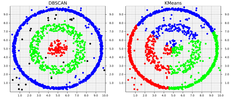
- Avoid if clusters have highly varying densities (use HDBSCAN instead).
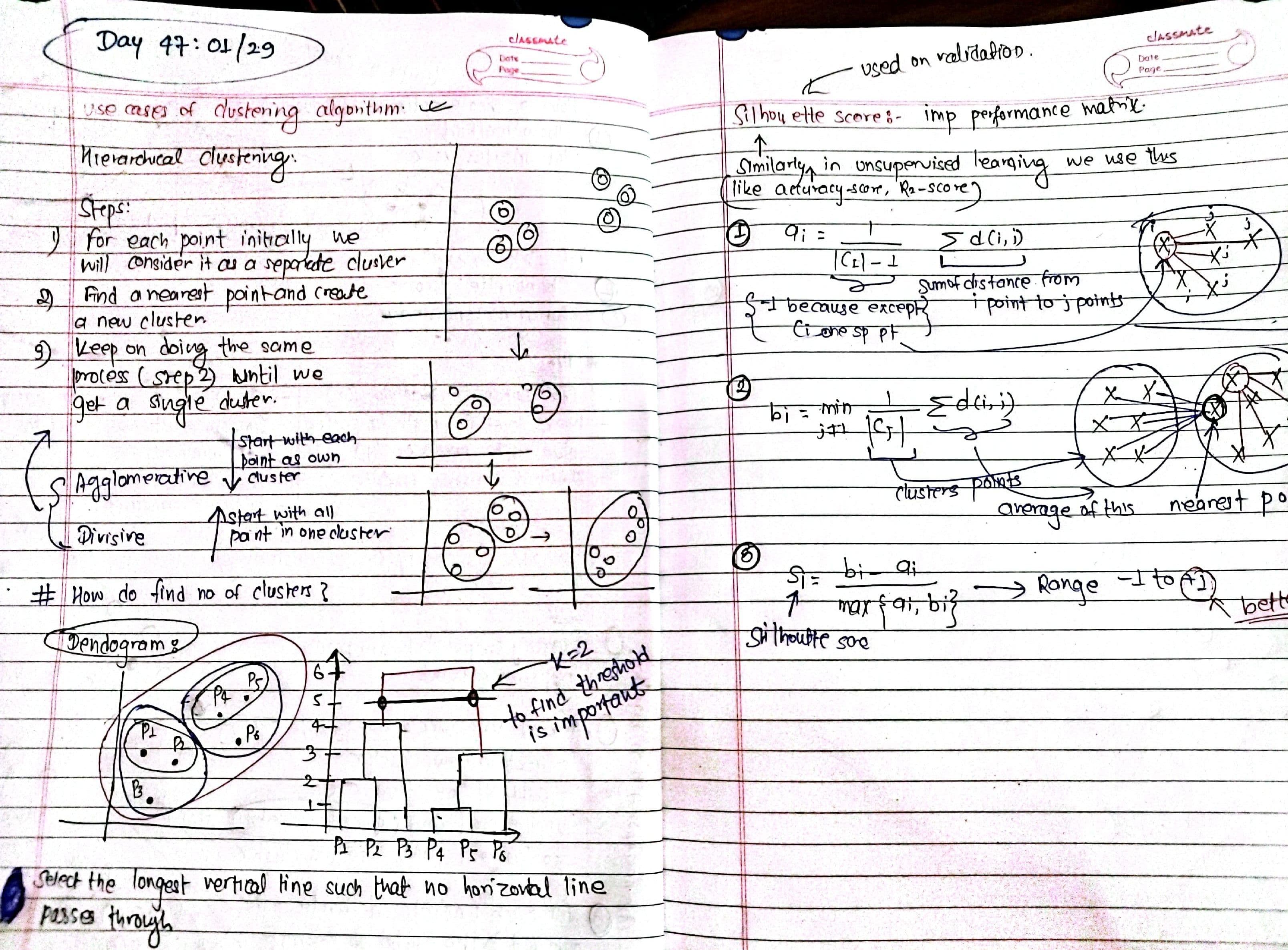
Day 47: Hierarchical clustering, Silhouette score
Hierarchical Clustering
Hierarchical clustering builds a tree-like hierarchy (dendrogram - a tree diagram showing how clusters merge/split. height shows the distance of merging, and cutting at a height defines the number of clusters.) of clusters. Two main approaches:
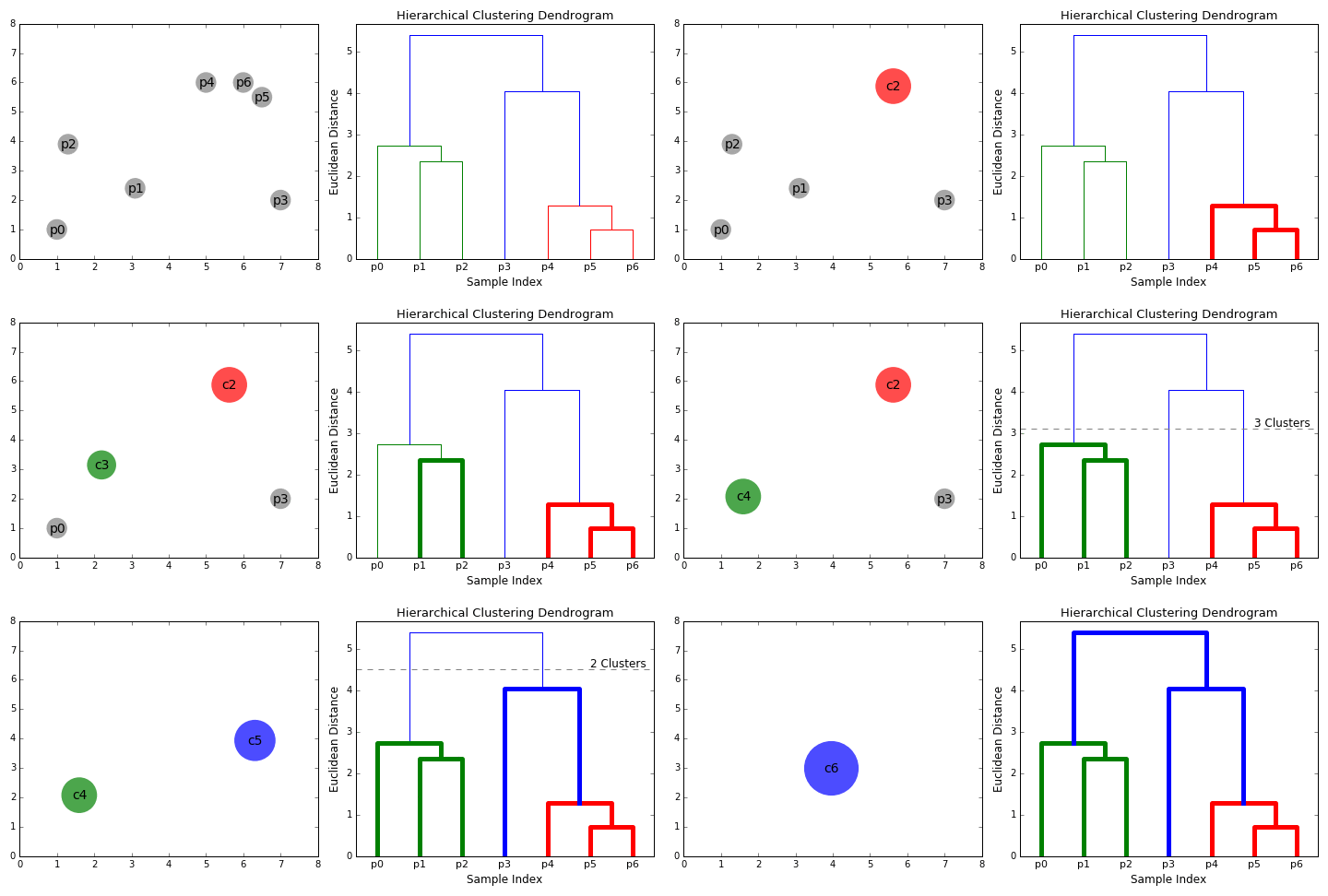
- Agglomerative (Given below): Start with each point as its own cluster, iteratively merge closest clusters.
- Divisive (Reverse of Agglomerative): Start with all points in one cluster, recursively split into smaller clusters.
Agglomerative Clustering Steps:
- Initialize: Treat each data point as a singleton cluster.
- Compute Distance Matrix: Measure pairwise distances (e.g., Euclidean, Manhattan).
- Merge Clusters: Combine the two closest clusters; update the distance matrix.
- Repeat: Continue merging until one cluster remains.
| Pros | Cons |
|---|---|
| No need to specify cluster count upfront | Computationally heavy (O(n³) time, O(n²) space) |
| Dendrograms aid visualization | Sensitive to noise/outliers |
| Works well for small/mid-sized data | Merges are irreversible (local optima) |
Linkage Criteria
Defines how distances between clusters are calculated:
- Single Linkage: Minimum distance between clusters (prone to "chaining").
- Complete Linkage: Maximum distance (creates compact clusters).
- Average Linkage: Average distance between all pairs.
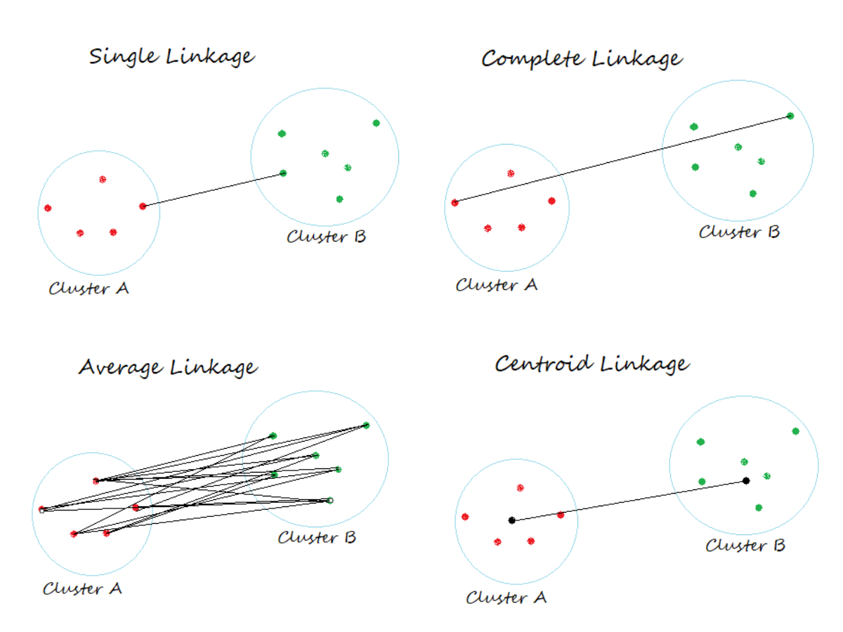
- Ward’s Method: Minimizes variance when merging (minimizes total within-cluster variance).
Silhouette Score
A metric to evaluate clustering quality by measuring how similar a data point is to its own cluster (cohesion) compared to other clusters (separation).
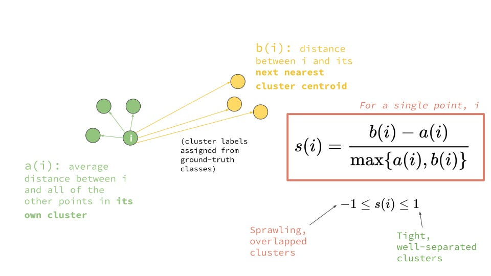
- Range: −1 (poor clustering) to +1 (well-defined clusters).
Day 48: Dimensionality Reduction
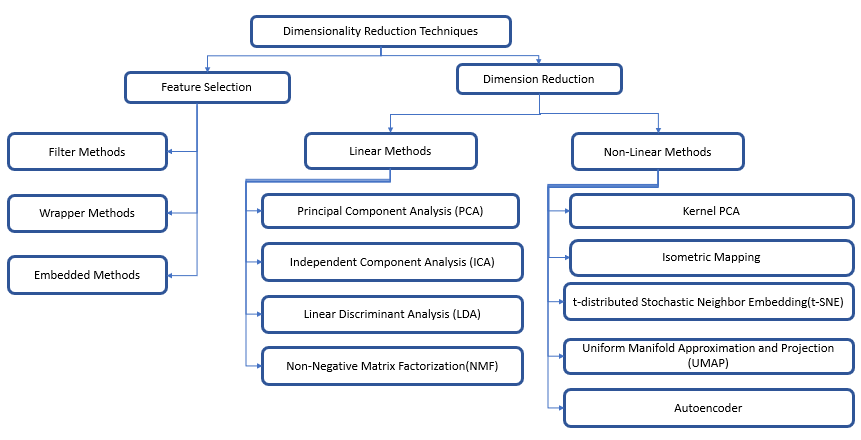
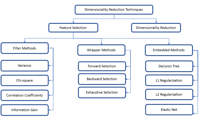
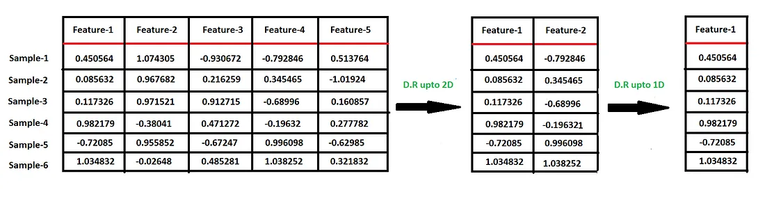
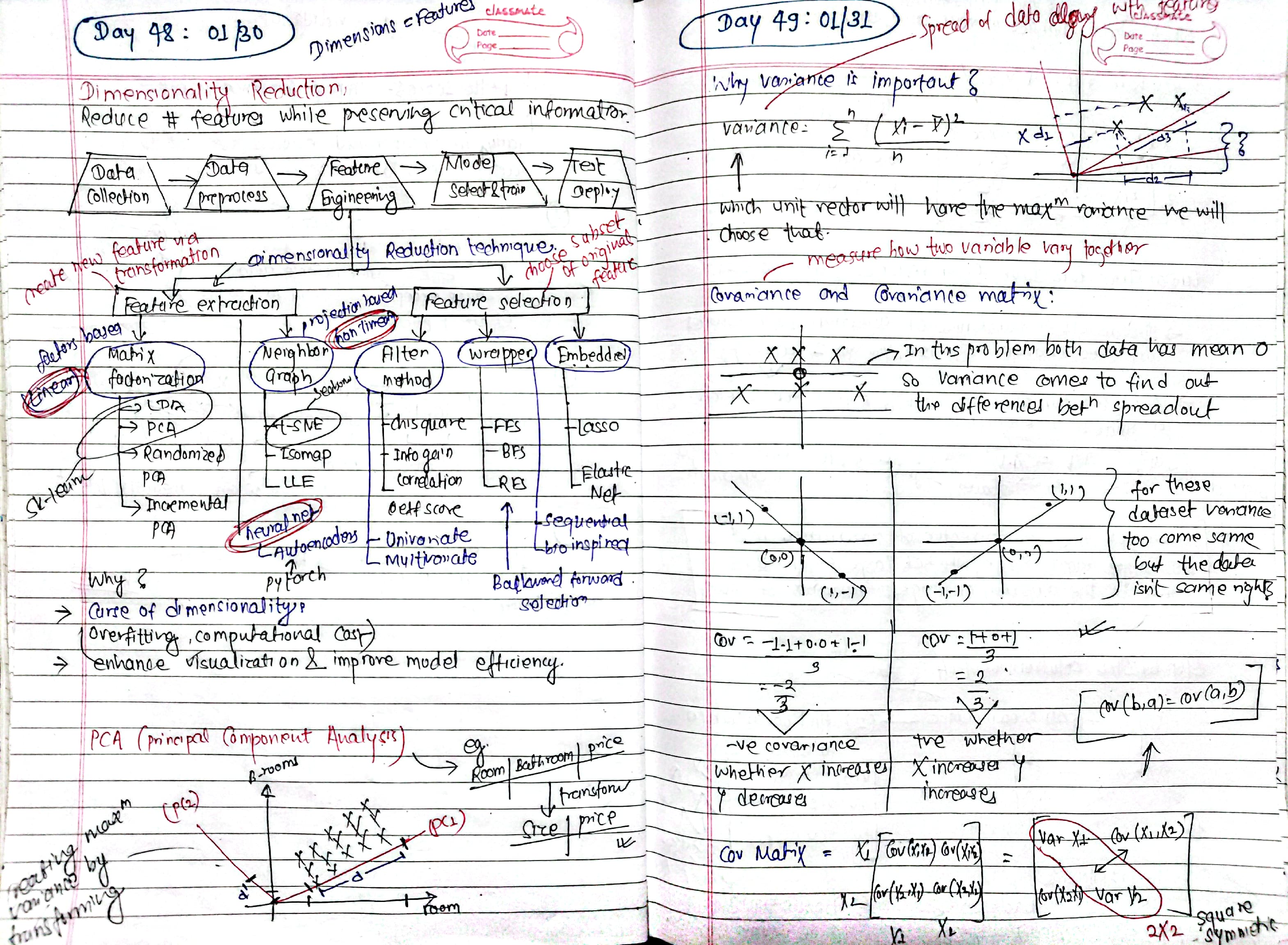
Reduces the number of features in data while retaining meaningful patterns, addressing noise, computational cost, and visualization. Methods are hierarchically grouped into feature selection (keeping relevant features) and feature extraction (creating new features).
Dimensionality Redduction Hierarchy:
 Feature Selection:
Dimensionality Reduction of a Data:
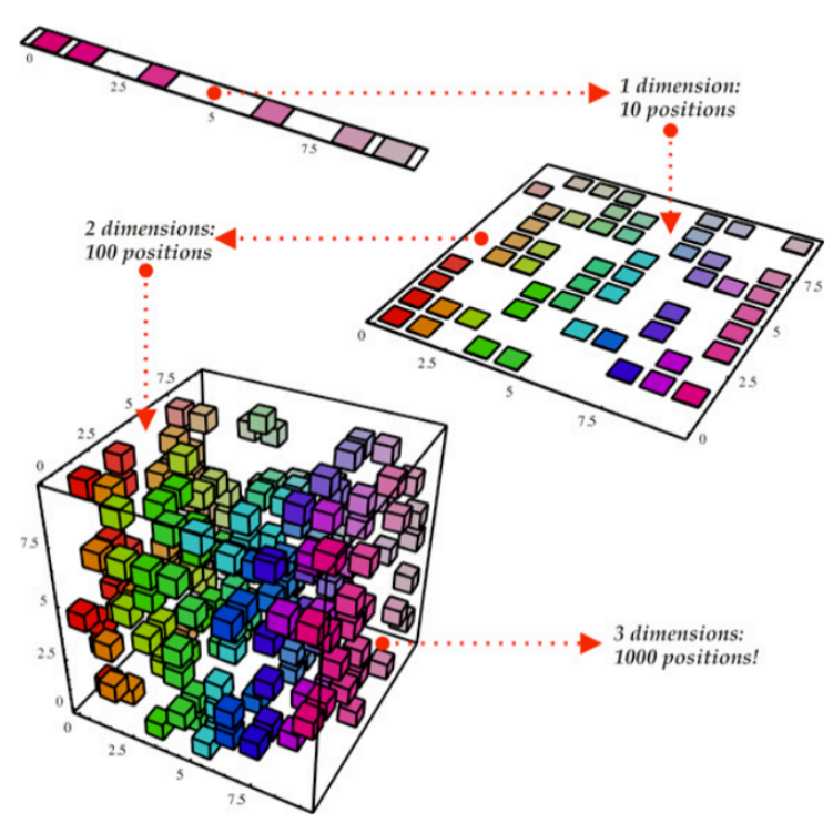
- Curse of Dimensionality: The curse of dimensionality refers to the challenges and inefficiencies that arise when analyzing data in high-dimensional spaces, such as sparsity, computational complexity, and loss of meaningful patterns.
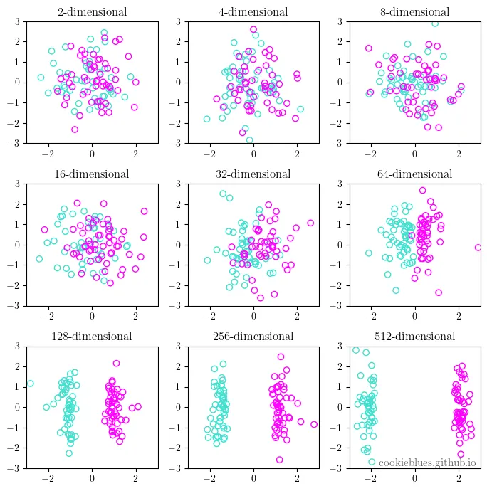 fig: As the dimensionality of data increases, the feature space becomes sparser, and the data is easier to separate. This is the curse of dimensionality in a nutshell.
Day 49: PCA (Principle Component analysis), Implementing with MNIST dataset
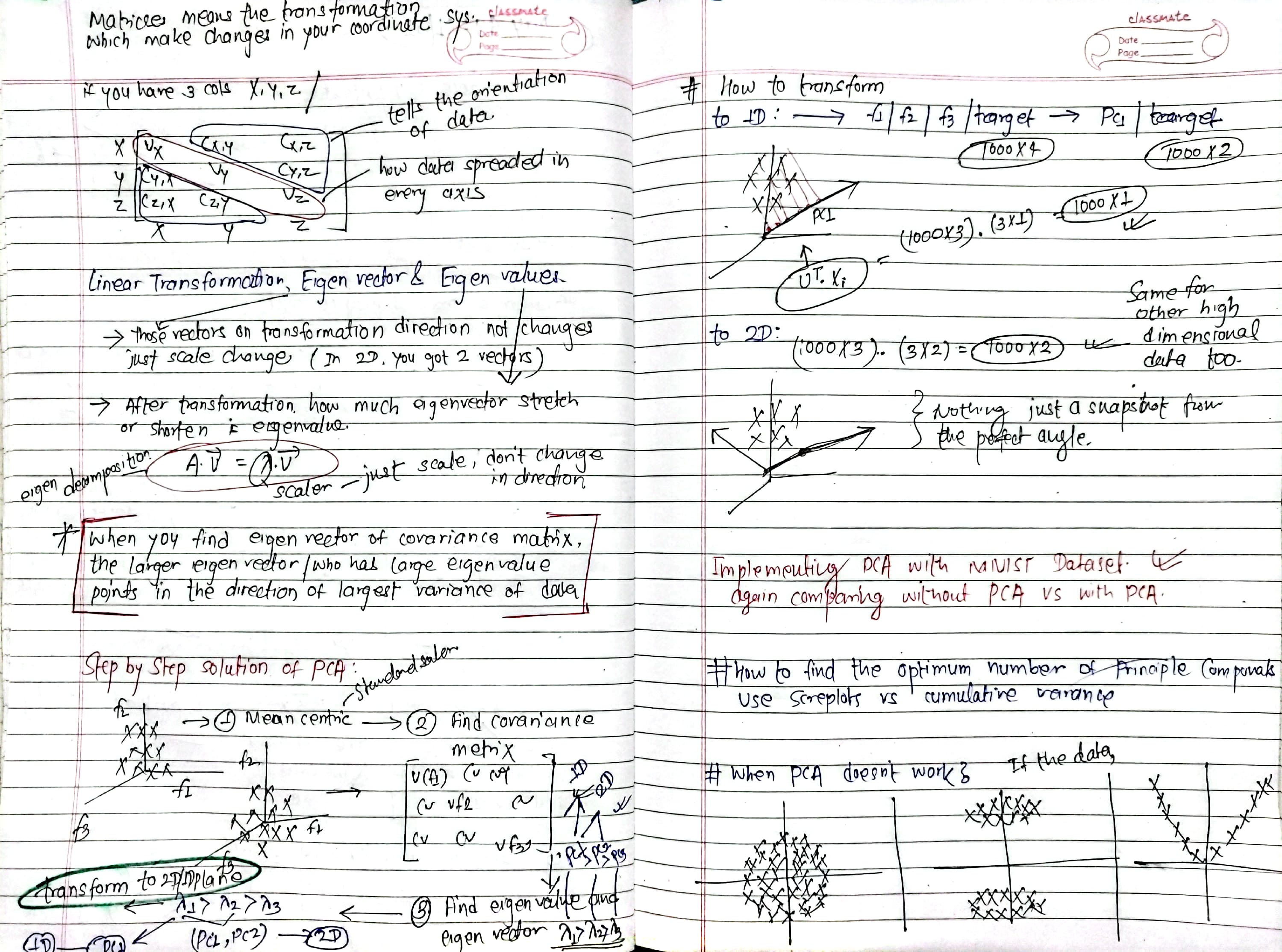
Goal: reduce dimensions while preserving maximum variance.
fig: pca projecting 2d data into 1d pc.
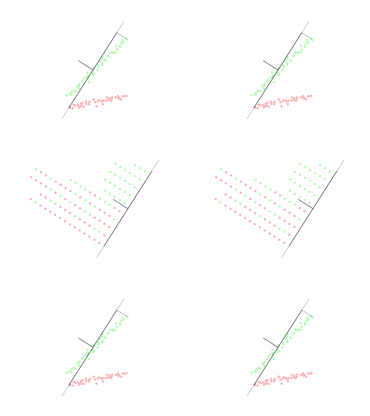
Example: Reducing 10D data to 2D → Use top 2 eigenvectors (highest eigenvalues).
Key Concepts
- Variance: Spread of data along a feature.
- Covariance: Measures how two variables vary together.
- Eigenvectors: Directions of maximum variance (principal components).
- Eigenvalues: Magnitude of variance along eigenvectors.
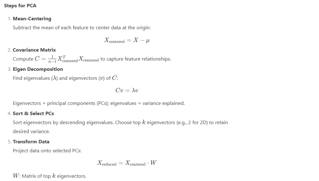
- Transformation: Project data onto new axes (eigenvectors) to reduce dimensions.
Steps →
How to choose the Optimal PC??
- select the optimal number of pcs by checking the cumulative explained variance, aiming to retain 90%-95% of the total variance, or by using the elbow method on the explained variance plot where additional pcs add minimal value
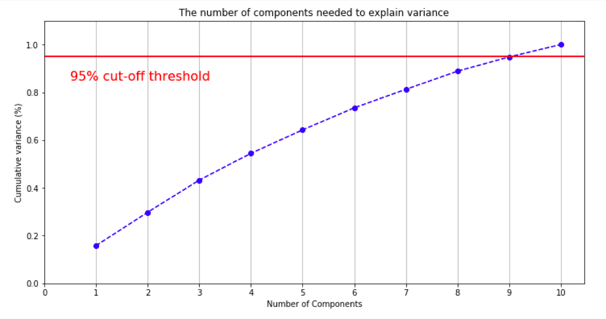 Notes:
Visualizing MNIST dataset on 2D and 3D:
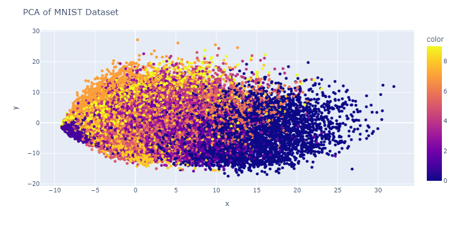
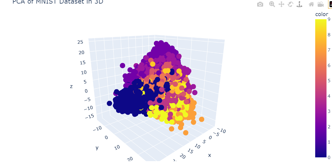
Notebook: Applying PCA on MNIST dataset
Conclusion: With about 100 PCs, our model predicts an accuracy of approximately 96%. In comparison, other models like KNN predict around 97% because KNN can capture more complex patterns in the data.
Day 50: Visualizing and Comparing PCA, t-SNE, UMAP, and LDA + Revision with the course ML specialization:
Today was a bit hectic as I tried to understand and visualize various dimensionality reduction techniques. Here's a summary of my learnings and comparisons:
Final Thoughts
- t-SNE: Captures local similarities well but sometimes distorts the global structure.
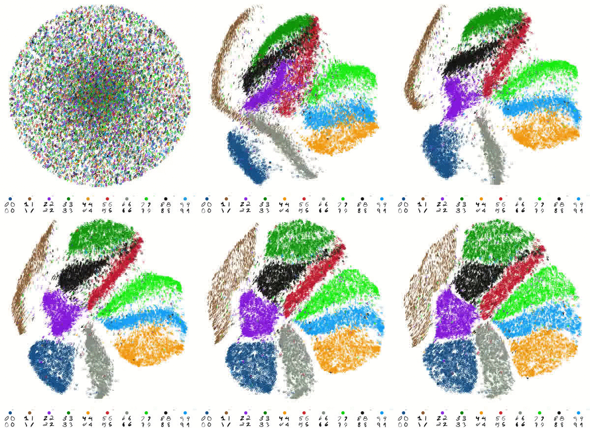
- UMAP: Faster than t-SNE and preserves both local and global relationships better.
- LDA: Supervised technique, works best when class separation is important.
Comparisons
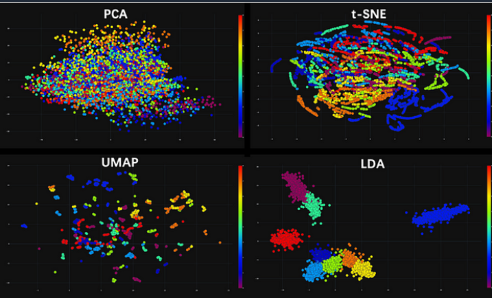
We explored four dimensionality reduction techniques for data visualization: PCA, t-SNE, UMAP, and LDA. We used them to visualize a high-dimensional dataset in 2D and 3D plots.
Note: It's easy to fall into the trap of considering one technique better than the other. At the end of the day, there's no perfect way to map high-dimensional data into low dimensions while preserving the entire structure. There's always a trade-off in the qualities each technique offers.
Resources
- Notebook: 3D Visualizations of PCA, t-SNE, UMAP, LDA
- Article: Dimensionality Reduction for Data Visualization: PCA vs t-SNE vs UMAP
Comparison of Results on MNIST
| Technique | Local Structure | Global Structure | Supervised? | Example Result |
|---|---|---|---|---|
| t-SNE | Preserved | Not preserved | No | Tight clusters of "2"s and "7"s, but arbitrary spacing between clusters. |
| UMAP | Preserved | Partially preserved | No | Tight clusters of "2"s and "7"s, with meaningful spacing between clusters. |
| LDA | Preserved | Preserved (class separation) | Yes | Distinct groups for each digit, optimized for classification. |
The learning is so hectic today, so I decided to revise the concepts we studied today with the help of Andrew NG. Here's the revision:
- What is clustering?
- Clustering is grouping data points into clusters where points in the same cluster are more similar to each other than to those in other clusters.
- K-means?
- K-means is a clustering algorithm that partitions data into K clusters by minimizing the distance between data points and their respective cluster centroids.
- optimization objective?
- The goal is to minimize the sum of squared distances between data points and their nearest cluster centroid.
- Lab?? done// Notebook: Lab Assignment
Day 51: Anomaly Detection:
What is Anomaly Detection?
- Identifying rare data points (anomalies) that deviate significantly from the majority of the data.
- Fraud detection, system failure prediction, intrusion detection, healthcare monitoring.
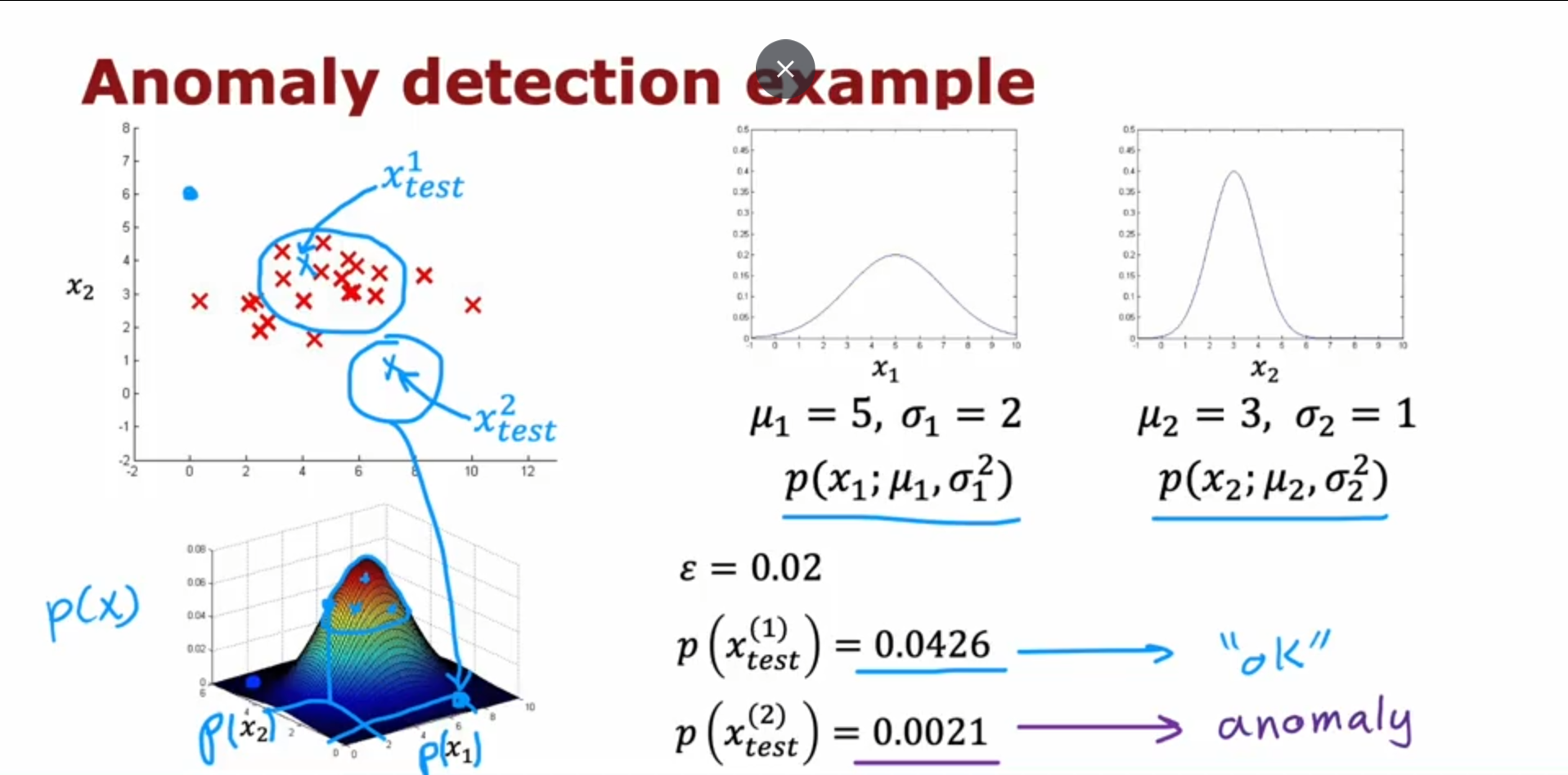
Approaches for Anomaly Detection:
- Gaussian Distribution: Flag data points outside ±3σ (99.7% of data).
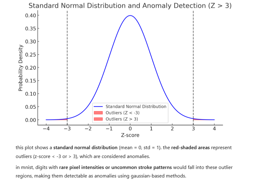
- Z-Score: Z=(x−μ)σZ=σ(x−μ); if ∣Z∣>3∣Z∣>3, mark as anomaly.
- Unsupervised:
- Clustering (K-means, DBSCAN): Anomalies lie far from cluster centers.
- Isolation Forest: Randomly splits data; anomalies are easier to isolate.
- Autoencoders: Neural networks that reconstruct input. High reconstruction error = anomaly.
Evaluation Metrics
- Precision: % of detected anomalies that are real.
- Recall: % of true anomalies detected.
- F1-Score: Harmonic mean of precision and recall.
- ROC-AUC: Measures trade-off between TPR (recall) and FPR.
Choose Algorithm:
- Small data? Use statistical methods (Z-score).
- Large data? Try Isolation Forest or Autoencoders.
Notes:
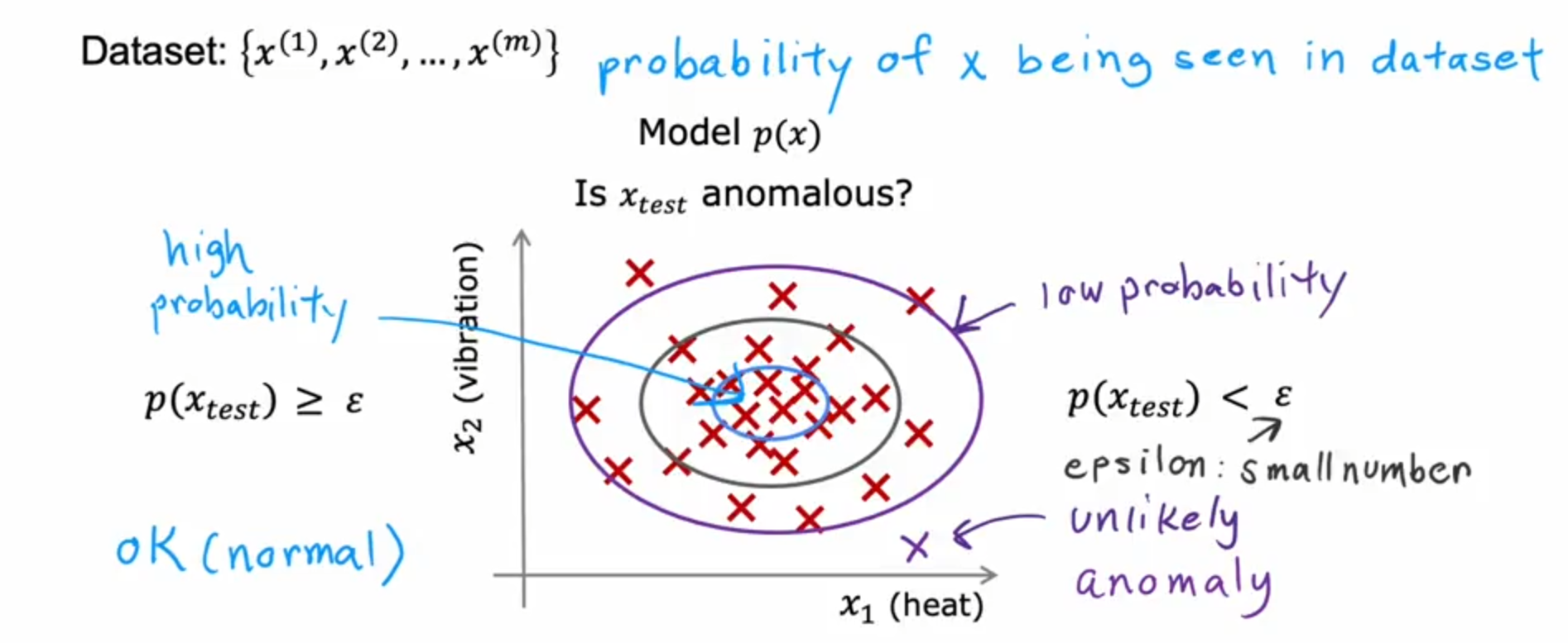
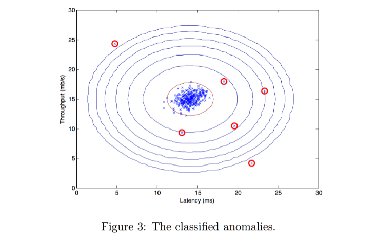
- Assuming data is normally distributed.
- Ignoring temporal/spatial context (e.g., seasonal trends).
- Not updating models as data evolves.
Day 52: collaborative filtering
Best Article (Working behind CF): https://medium.com/@ashmi_banerjee/understanding-collaborative-filtering-f1f496c673fd
Collaborative Filtering is a recommendation algorithm that considers the similarities between different users when recommending an item to another user.
Making Recommendations
- Predict what a user might like based on similar users/items.
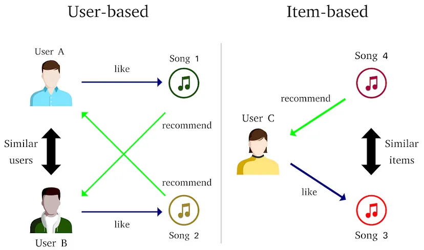
- User-User CF: Find users like you → recommend what they liked.
- Item-Item CF: Find items similar to what you liked → recommend those.
the approach minimizes a regularized cost function using gradient descent, adjusting user and item parameters iteratively. the learning rate (α) controls step size, balancing convergence speed and stability.
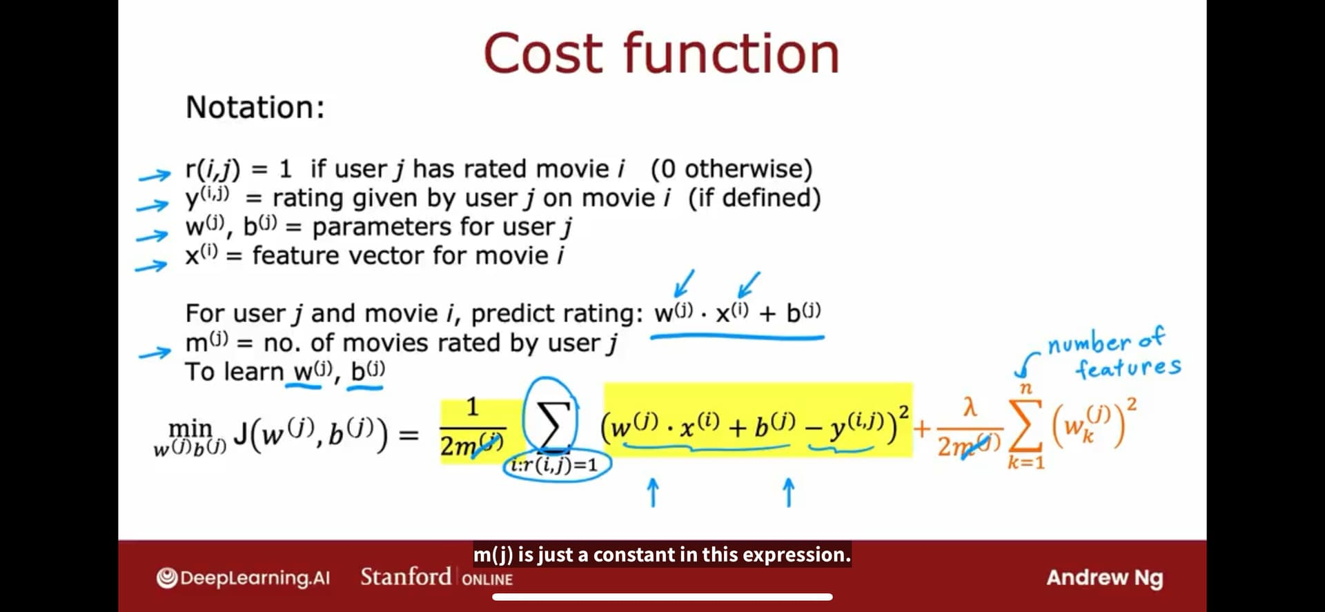
while effective, it suffers from the cold start problem (new users/items lack data) and sparsity issues (many missing ratings). despite these challenges, it remains a widely used technique in recommender systems.
Mean Normalization
- Why? Handle users who rate everything too high/low.
Collaborative Filtering vs Content-Based Filtering
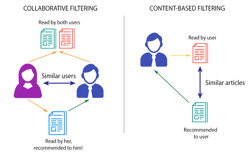
| CF | Content-Based |
|---|---|
| Uses user-item interactions | Uses item features (e.g., text, genre) |
| Example: Netflix recommendations | Example: News articles recommended based on text keywords |
Day 53: Project @ Football Players Market Value Prediction - Introduction and Planning
Inspired by the work of Youla Sozen
Every project starts with a problem or question. However, this project is different. it's all about having fun. As a football enthusiast, creating these kinds of projects is always enjoyable. The plan is straightforward, and I will implement it step by step.
Project plan
Although this is a fun project, i aim to ensure the following:
- accurate player valuation: estimating market values to benefit clubs, agents, and investors.
- transfer market efficiency: preventing overpayment, aiding negotiation, and optimizing resource allocation.
- risk assessment & player development: evaluating investments while identifying young talents with high growth potential.
- data-driven insights: supporting fairer contract negotiations and improving decision-making in fantasy football & betting.
this is a future plan, and i will work towards achieving these goals in the coming days.
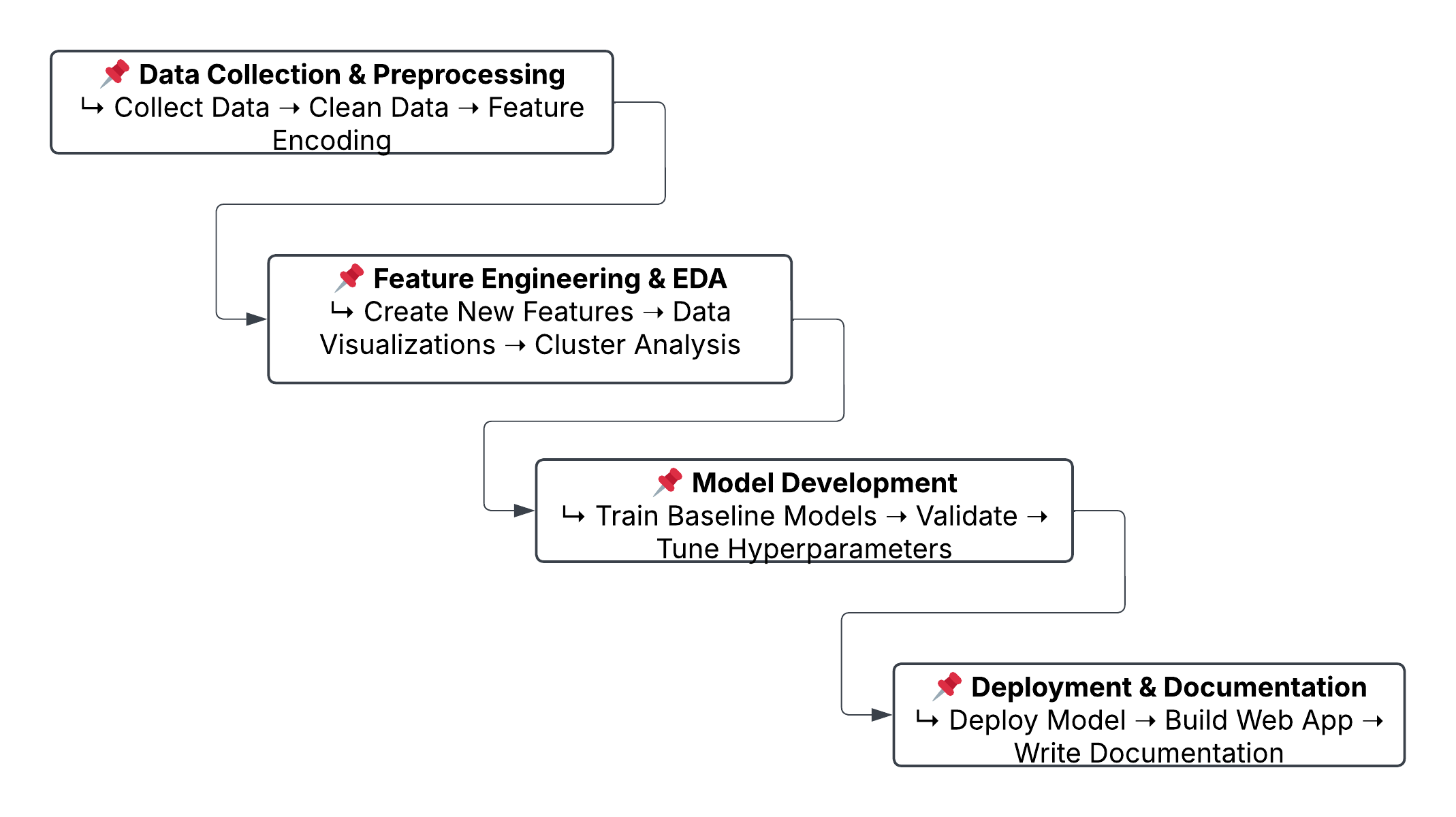
Tips for the project (crafted with deepseek):
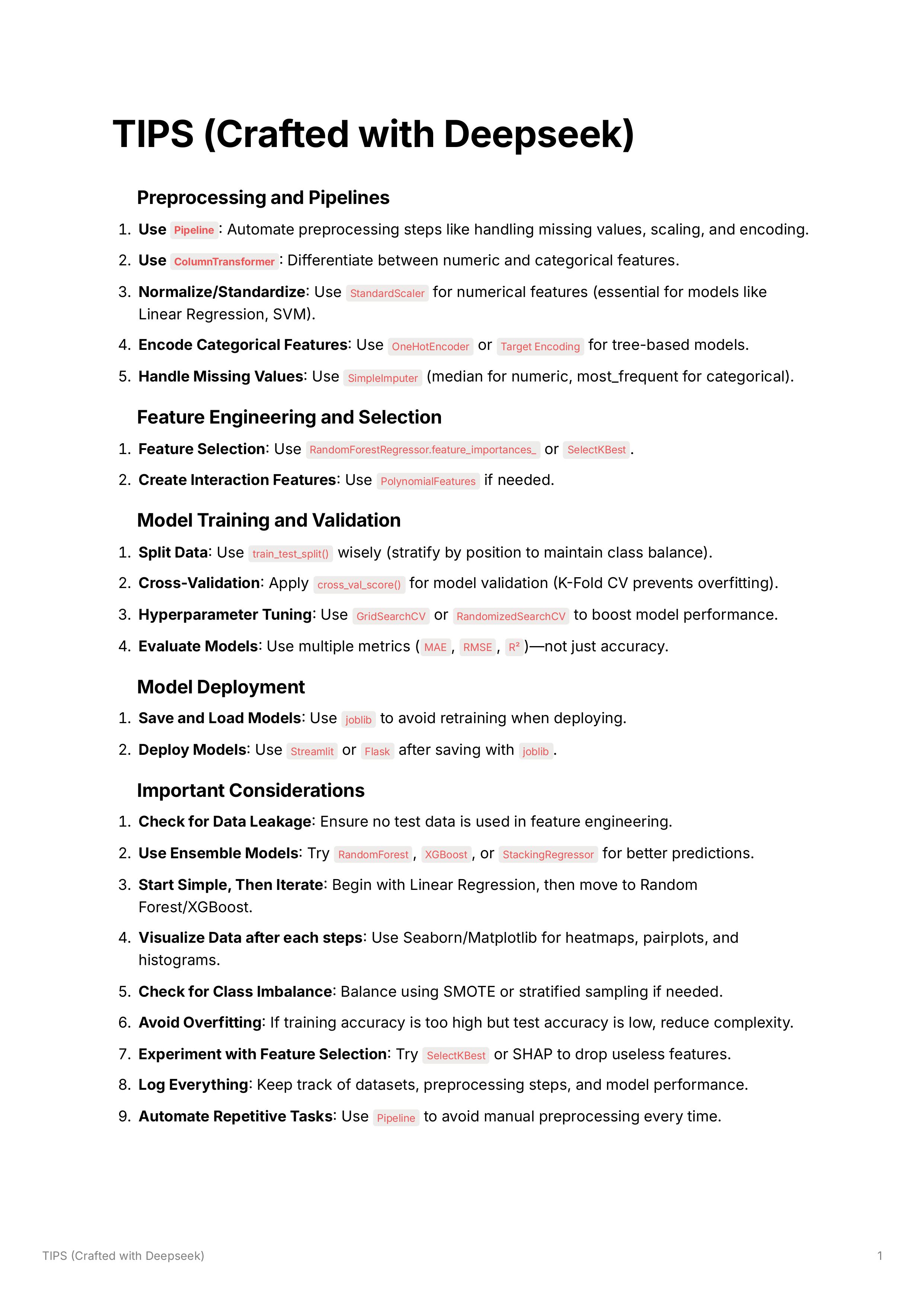
Day 54: Project @ Football Players Market Value Prediction - Collecting Data (Scraping)
web scraping is a technique to collect data from the internet and convert it into a meaningful format, like a data frame, when direct downloads aren't available. in this project, i used the sofifa dataset. here's the main page of sofifa
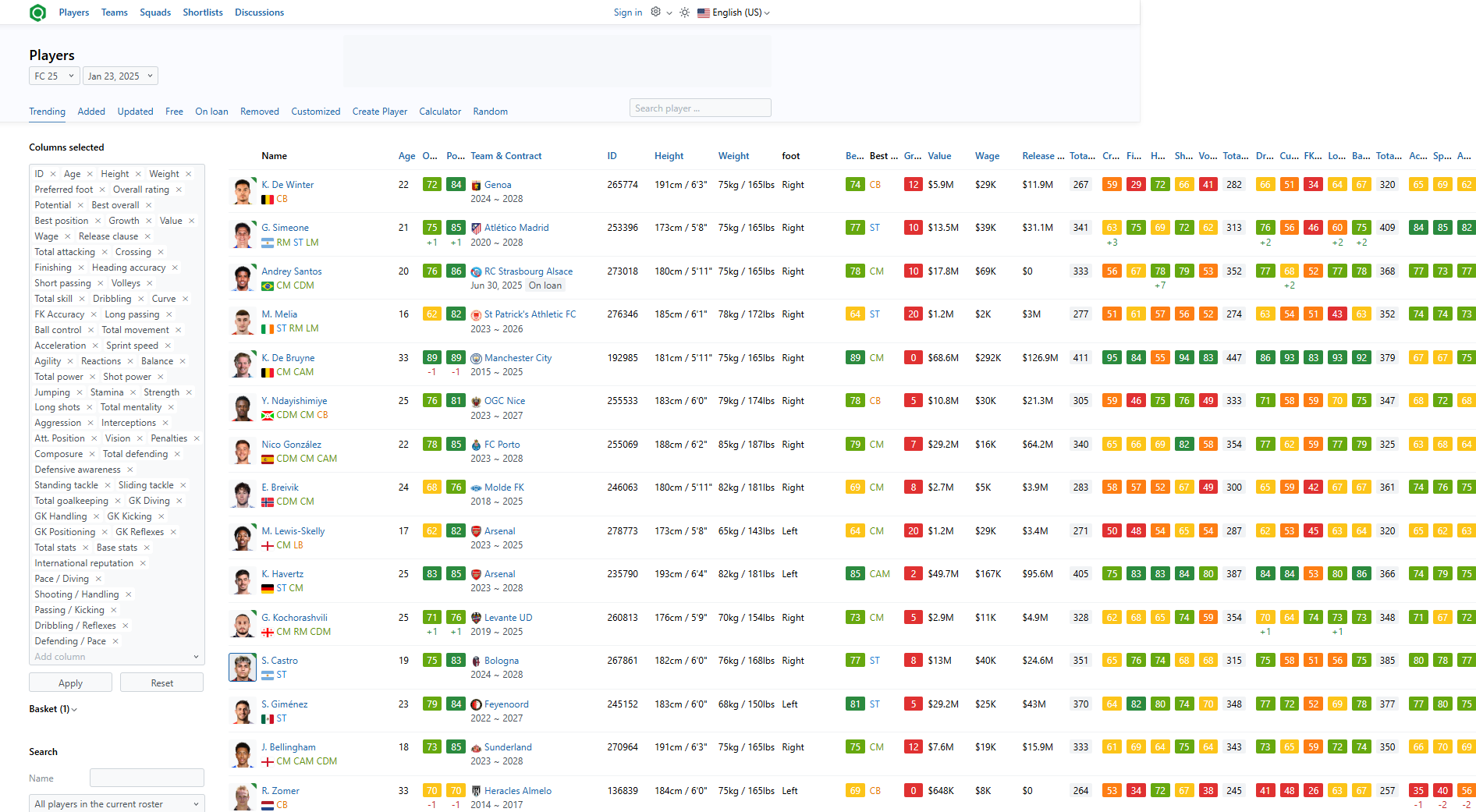
Code to scrape data:
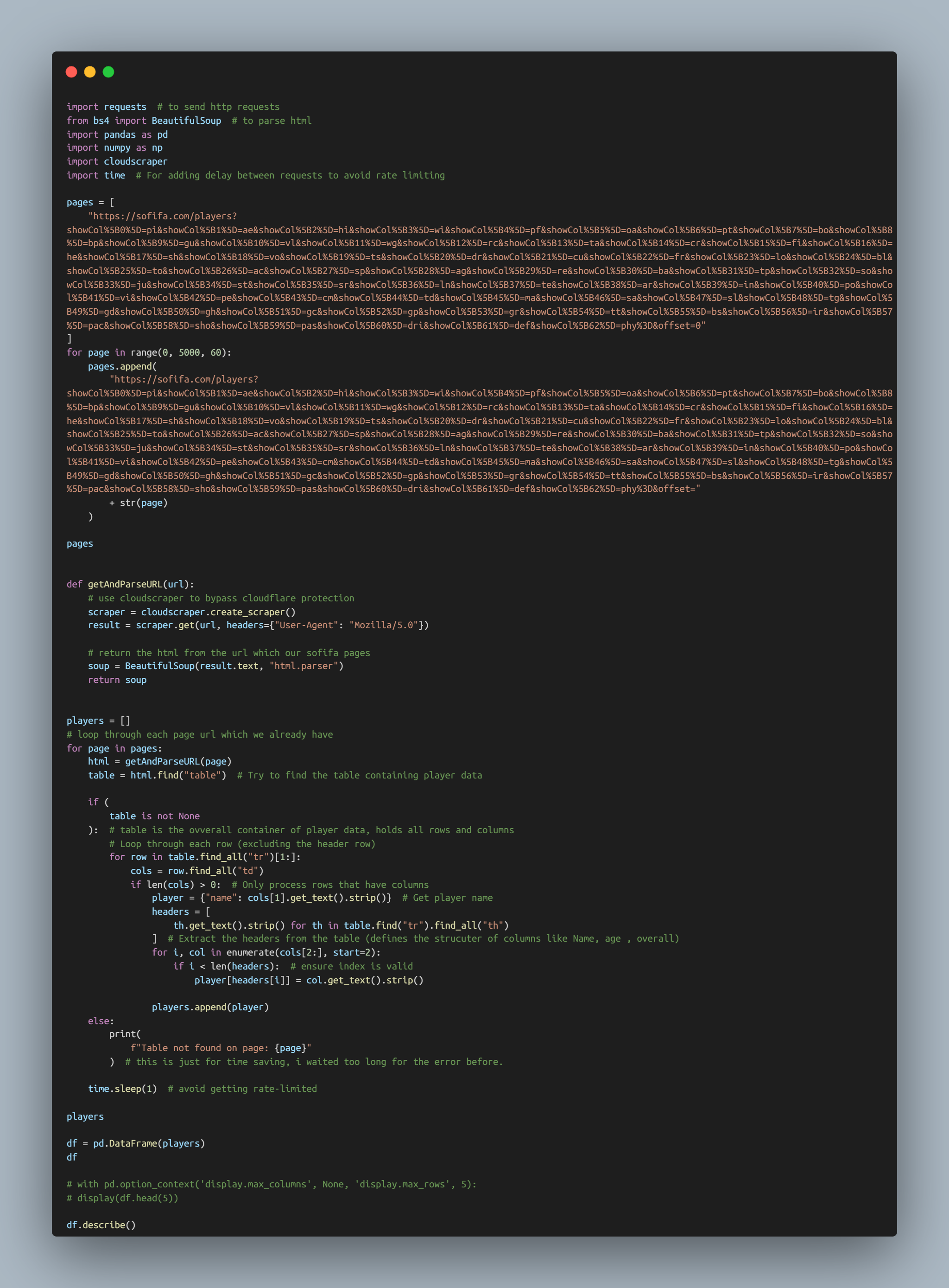
Plan for cleaning Data:
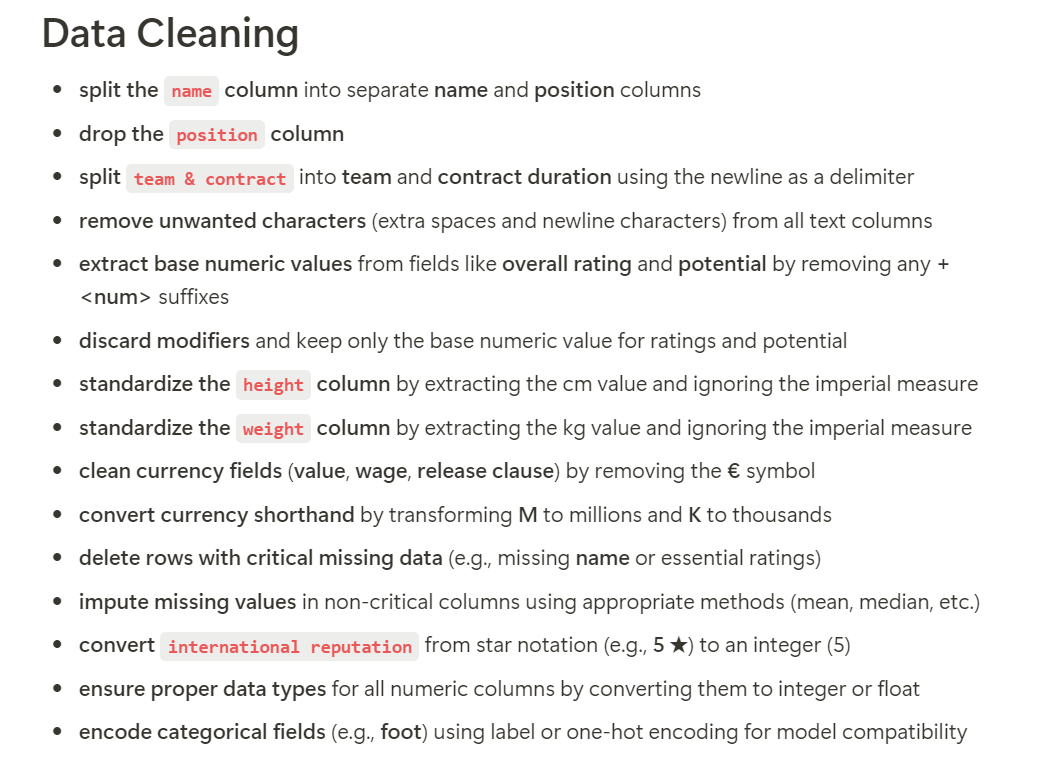
Day 55: Project @ Football Players Market Value Prediction - Cleaning Data
just finished a major data cleaning session for my project. went through steps like handling missing values, converting currencies, splitting combined columns (height/weight), and ensuring consistent data types. cleaned up outliers, removed duplicates, and made sure everything’s ready for the next phase: EDA and model training. feeling good with the progress 😁
Here's a final look: Notebook: Data Cleaning
Code:
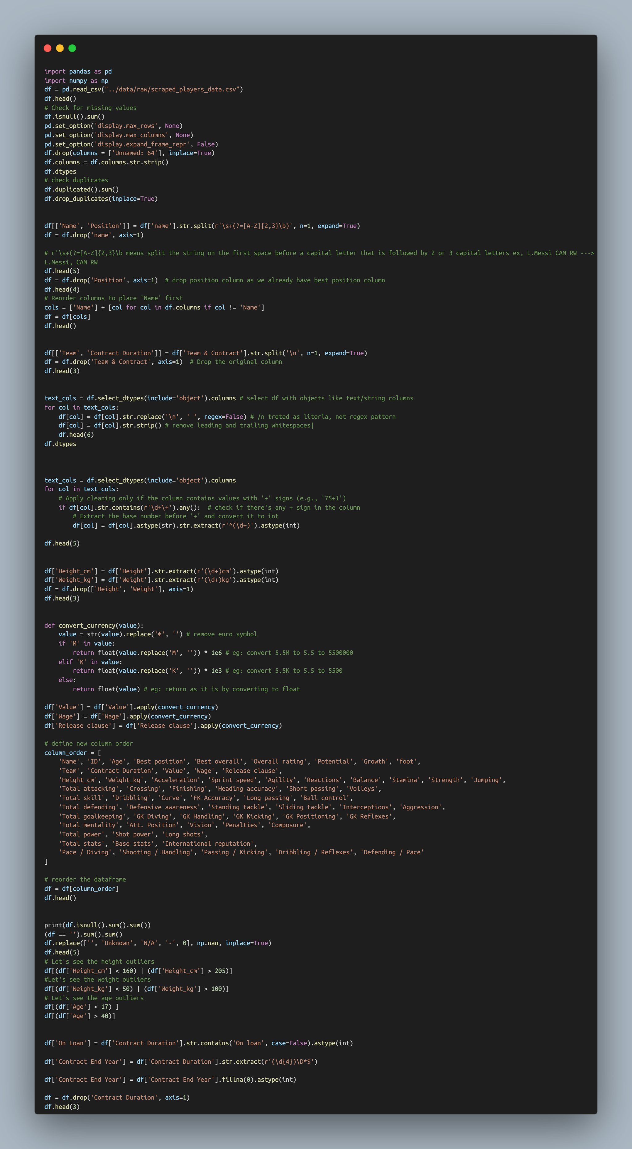
Day 56: Project @ Football Players Market Value Prediction - EDA
Notebook: EDA (With Complete Documentation)
I have mostly used Plotly to visualize as it is interactive and for such beginners like me, the visualization impact is powerful. as well as the codes are also easy to write.
overall dataset insights
- what are the top 10 most valuable players?
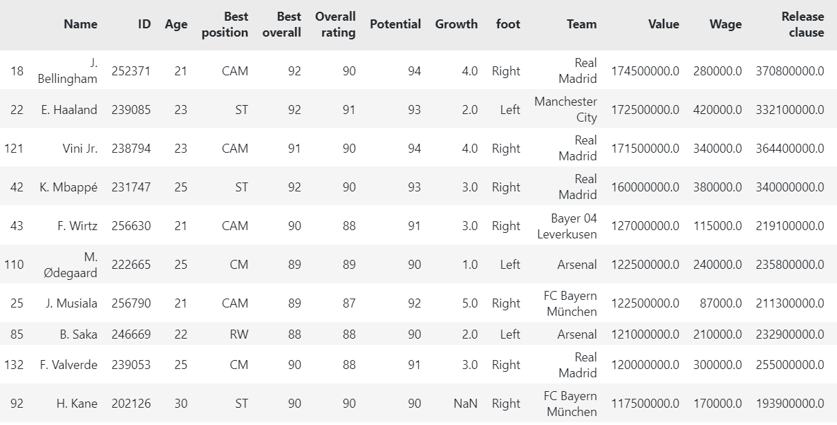
- how does market value vary by position (e.g., are strikers more expensive than defenders)?
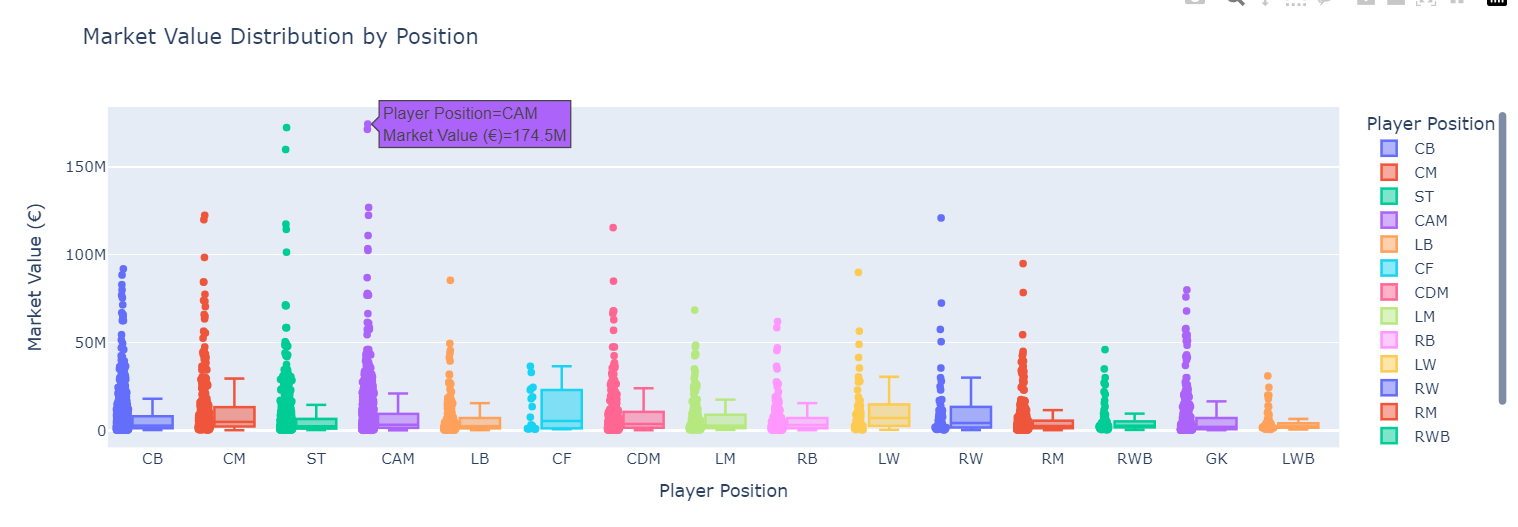
- which teams have the highest average market value?
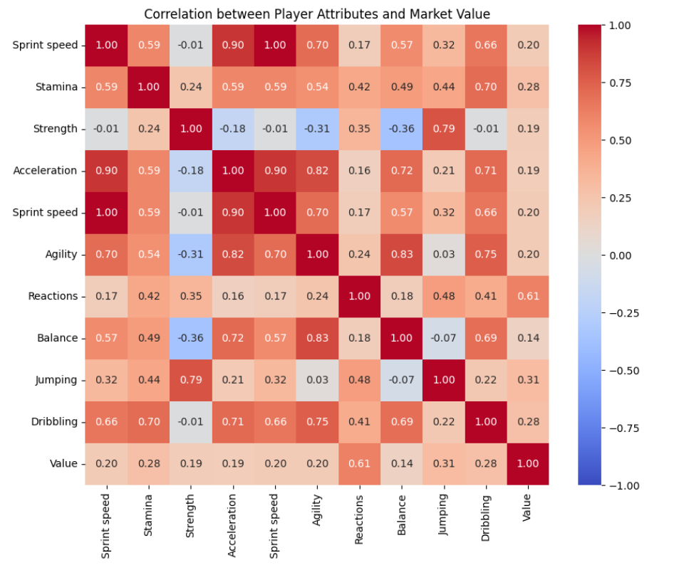
- what’s the distribution of market values (is it skewed towards a few expensive players)?
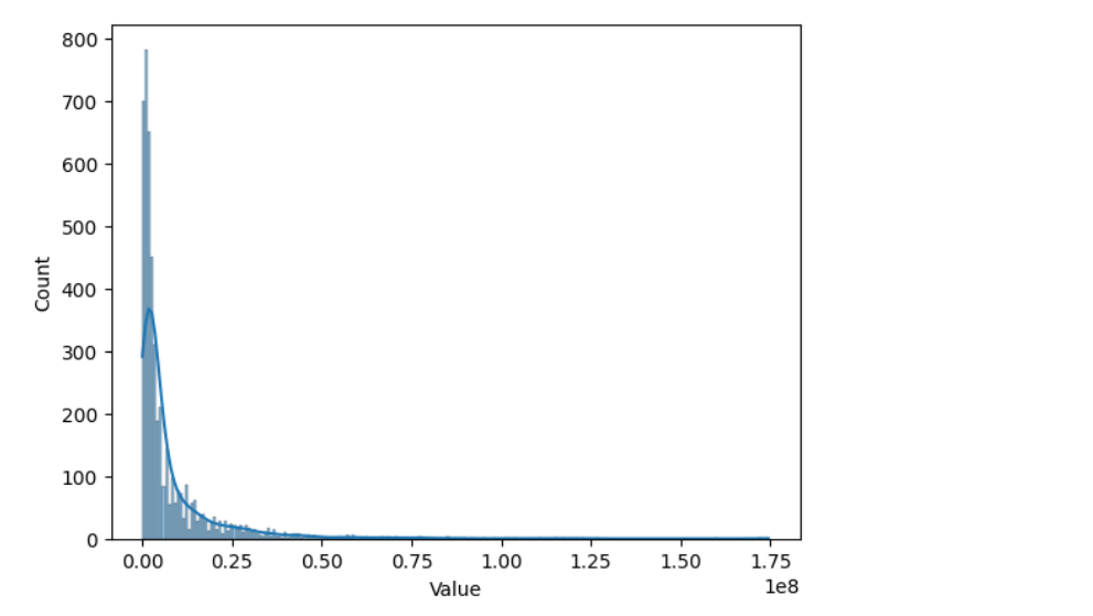
- how does age correlate with market value (are younger players generally worth more)?
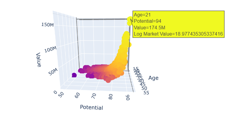
player attributes vs. market value
- how does a player’s overall rating affect their market value?
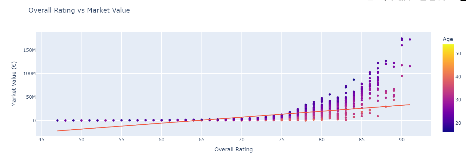
- which individual attributes (e.g., pace, stamina, strength) correlate the most with market value?
- does international reputation (1-5 stars) impact market value?
- how do potential ratings compare to market value (are high-potential players priced higher)?
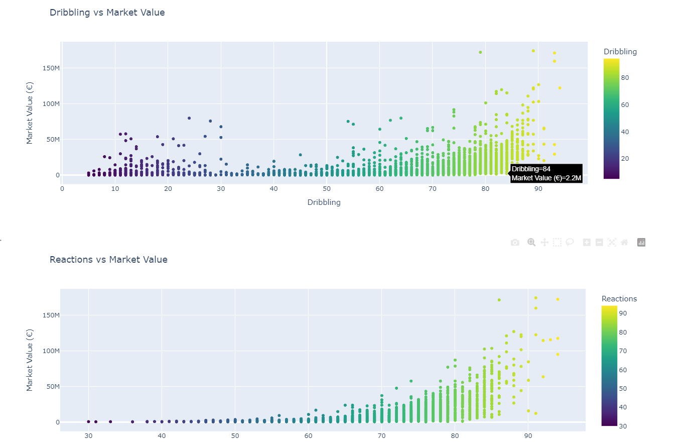
- do physical attributes (height, weight, strength) play a role in market value?
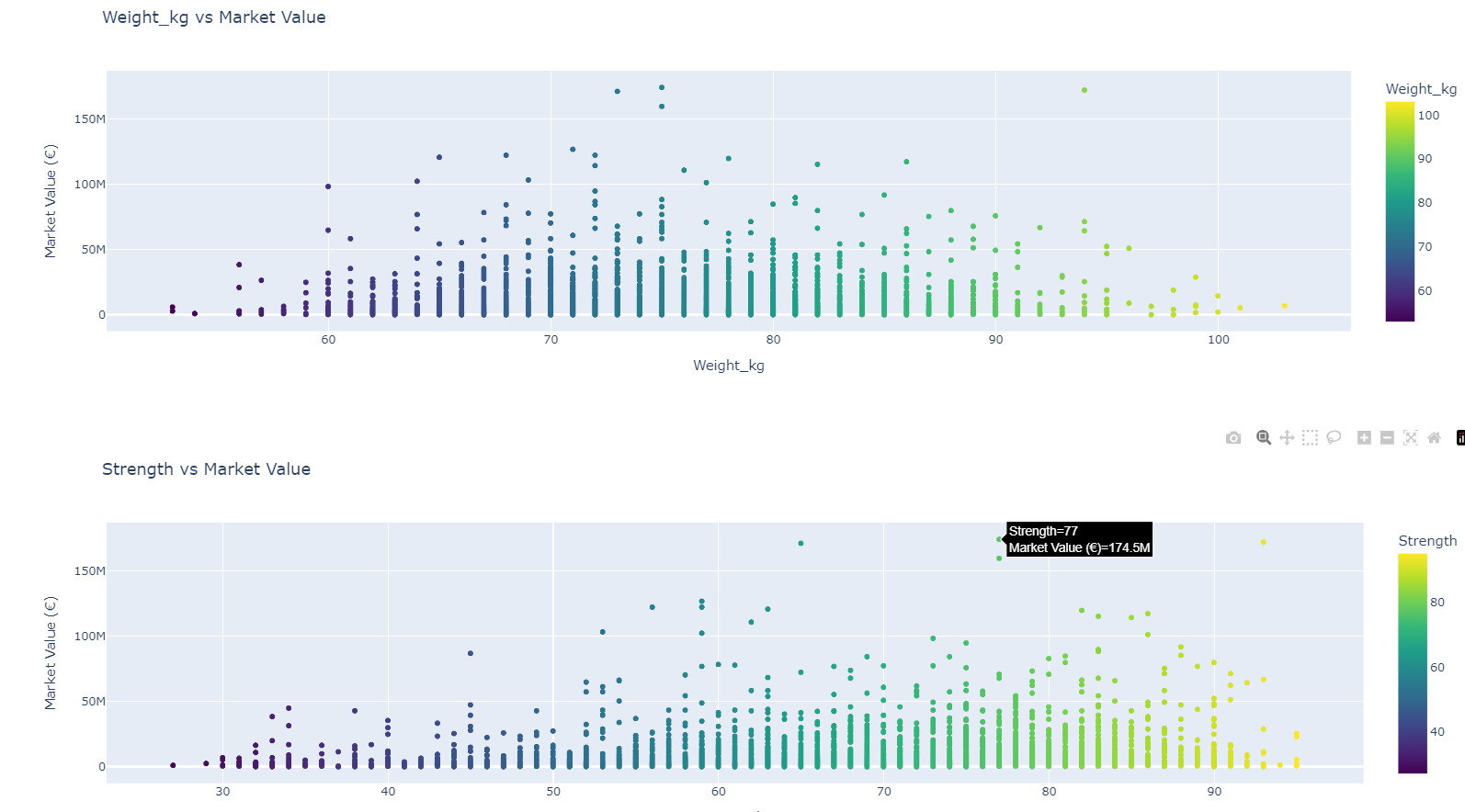
position-specific insights
- are attacking midfielders (CAM/CM) more valuable than defensive midfielders (CDM/CM)?
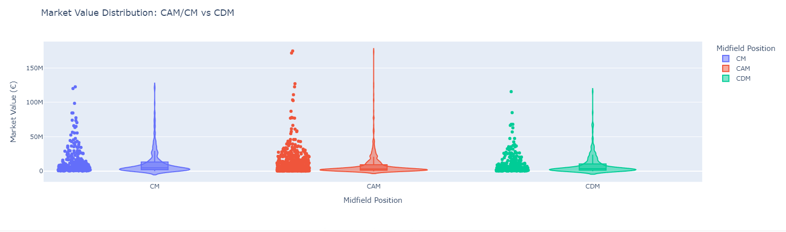
- how does pace affect wingers' (LW/RW) market value?
- do goalkeepers follow the same market trends as outfield players?
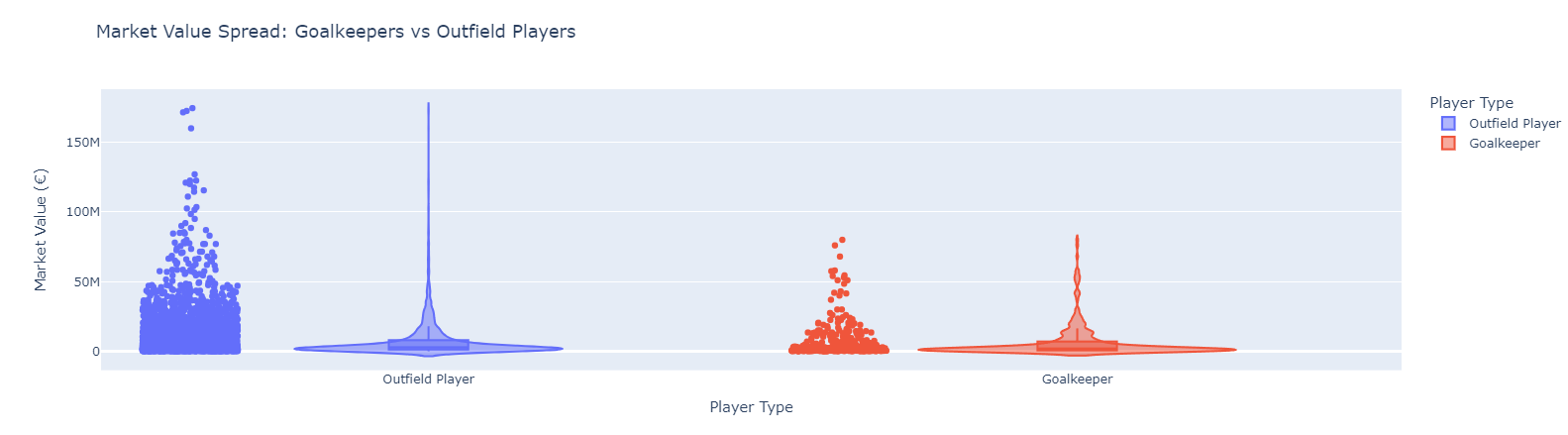
contract & transfer market impact
- does a player's contract end year affect their market value (e.g., do players with 1 year left have lower values)?
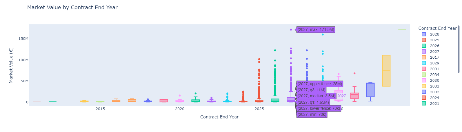
- are players on loan priced differently compared to permanent squad members?
Day 57: Project @ Football Players Market Value Prediction - Feature Engineering: (Creating features, Transforming Features)
Notebook: Creating and Transforming Features
spent 6+ hours experimenting with feature engineering. ran into some challenges, but made progress:
- position-based features: grouped players into categories (attackers, midfielders, defenders, goalkeepers) with scores. will refine tomorrow.
- club-based features: switched from one-hot encoding (curse of dimensionality) to target encoding using the mean market value for each club.
- contract-based features: correlation with market value was neutral. most features, except age, overall, and potential, seemed less important.
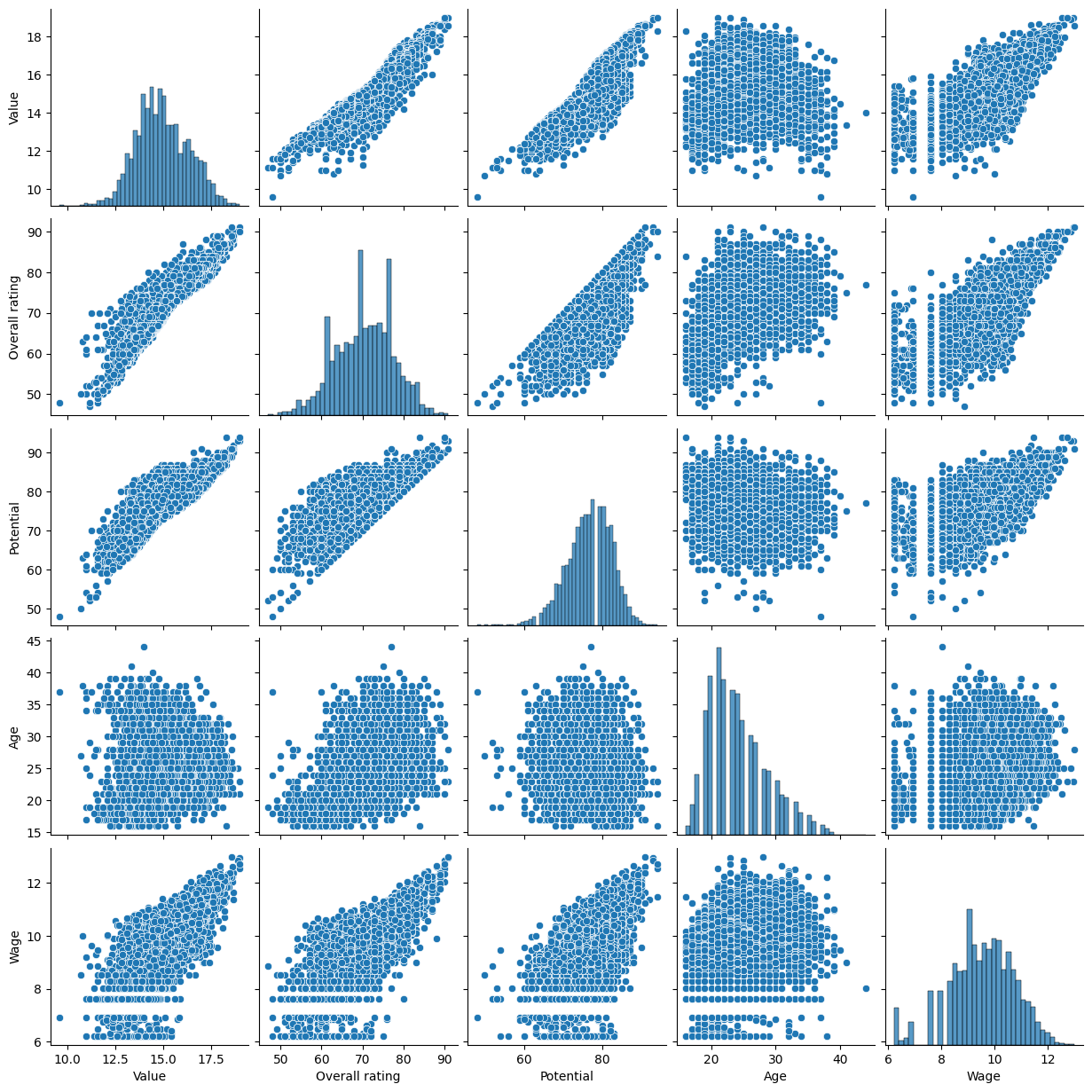
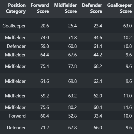
Day 58: Project @ Football Players Market Value Prediction - ML : (Linear Regression with Refined Features and deploying with Streamlit)
Just for fun:
Pairplots:
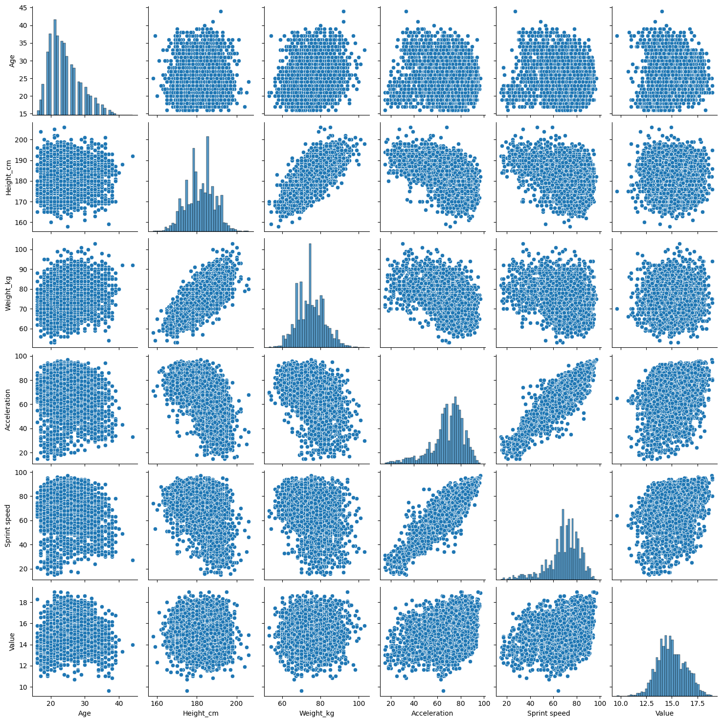
So, before diving into feature engineering after cleaning the data, i tried out linear regression and got an r2 score of around 0.52. then, after applying some feature engineering and playing around with features, i ran the same model and got the r2 score up to 0.96 with only numerical features
today, i wasn’t fully happy with the result and got confused about feature selection and engineering. so i decided to convert all features into numerical, applied scaling and transformation, and reran the model , r2 score shot up to 0.97
Saved the model immediately, then tried deploying it with streamlit locally, with a user input form and inverse transformations (MOST HATED PART) . while the model’s still a work in progress and not perfect, i'm proud of what i’ve learned so far. next steps are all about finding the best model and getting it deployed with some solid predictions and managing the form with the backend properly.
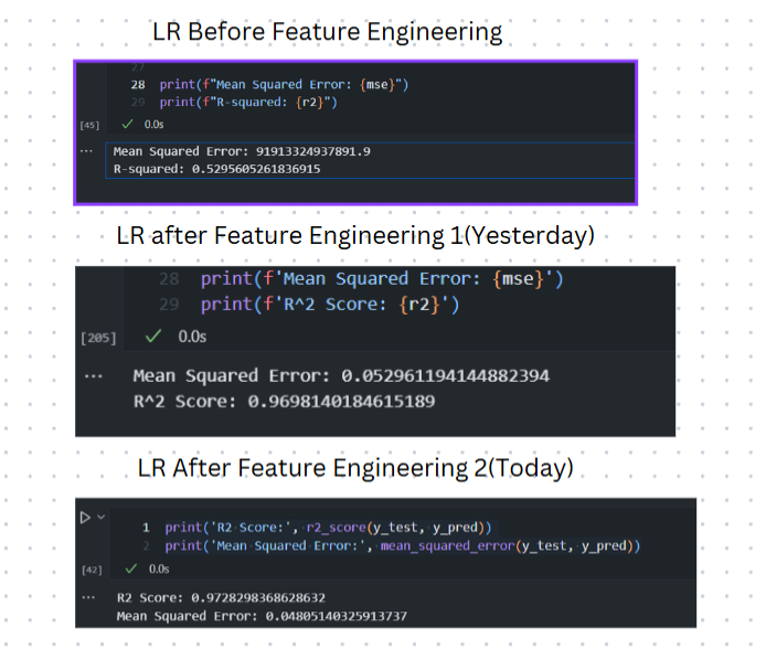
Streamlit Preview: https://www.linkedin.com/posts/paudelsamir_day-58365-linear-regression-with-refined-activity-7294398498777501697-2vWi?utm_source=share&utm_medium=member_desktop
Day 59: Project @ Football Players Market Value Prediction - Complete Streamlit Setup for our first Model - Linear Regression
Yesterday, I set up streamlit for my project with some help from ai tools. deploiyng isn't my strong suit, and it got pretty hectic trying to nail down the format and inputs and converting to model inputs. had to leave it unclear
So todayt's goal was get the ui sorted and code the input transformation for the model within streamlit. i could've tinkered with other models and tuned them, but finishing what i started felt right. a simple linear regression is doing surprisingly well for my needs. of course, i'll explore other algorithms and fine tune for better accuracy soon. planning to scale up from 5,000 to 20,000 rows in my dataset. let's see
Here's the demo where linear regression predicts player market values quite accurately. grabbed data from the site i scraped so that to visuailze properly. and its around 90 percent accurate for all the positions. that's already great !! Loving it
Here are some previewsL:
-
KDB (Real Vs Predicted)
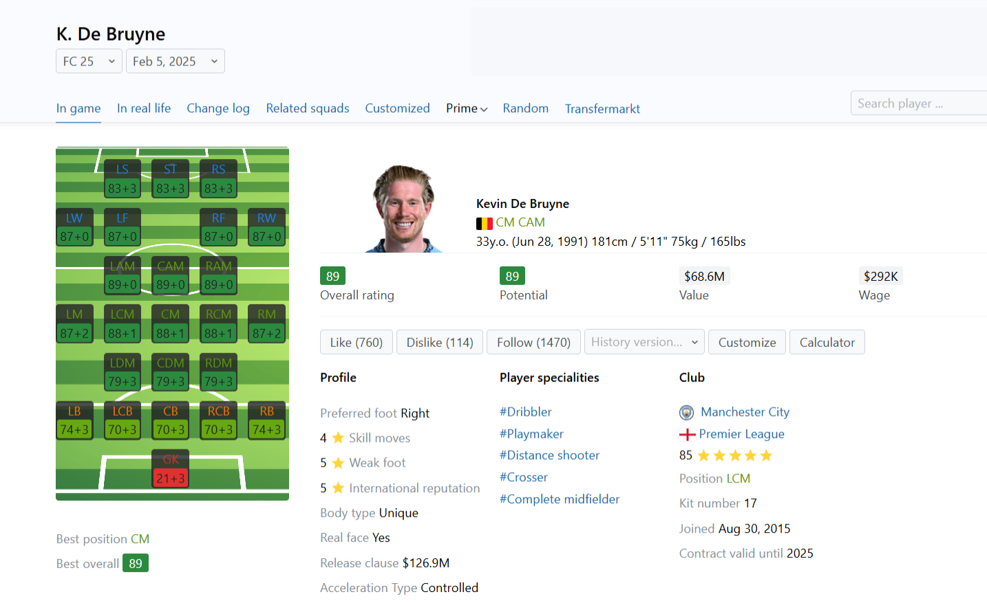

-
Lamine (Real Vs Predicted)
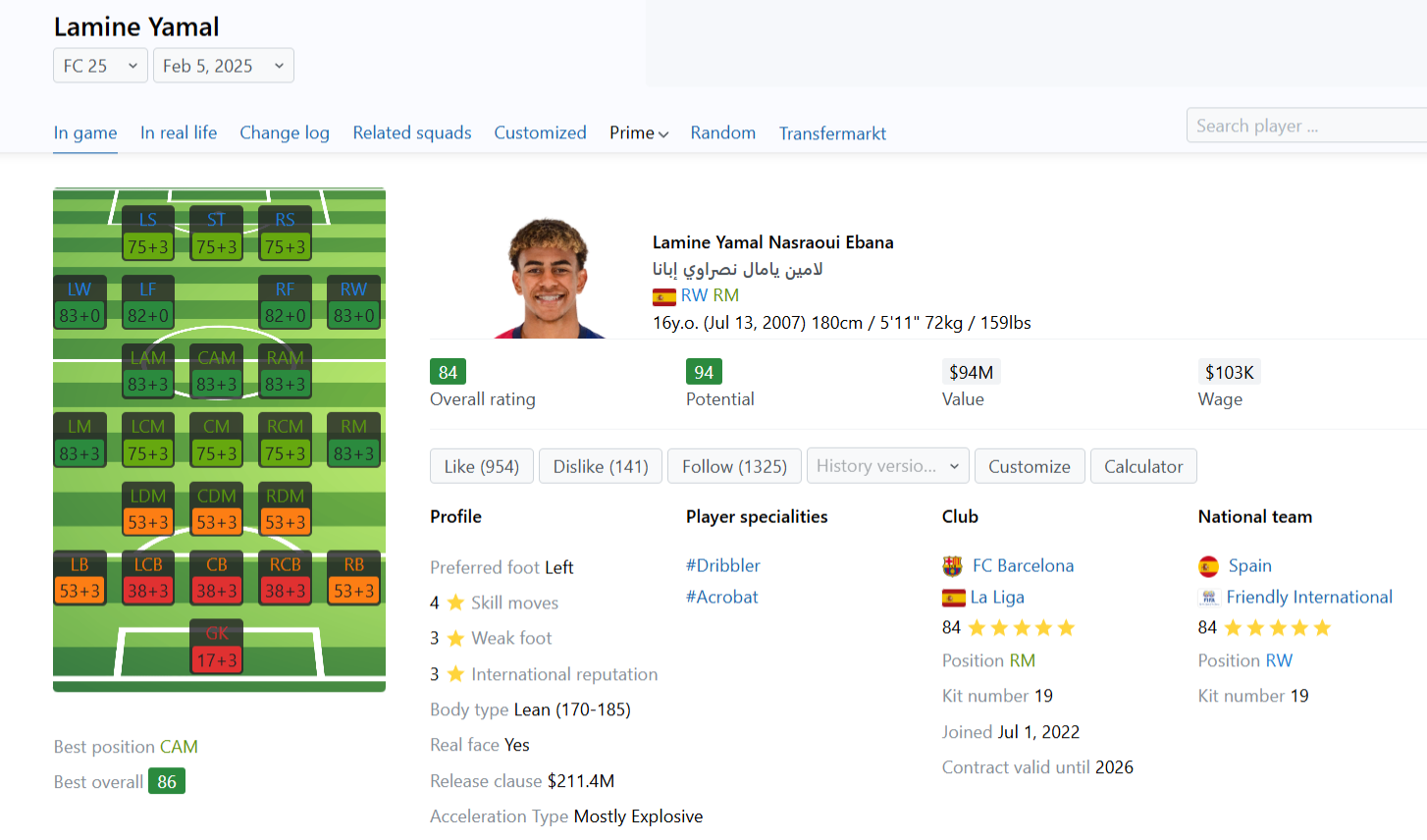

-
Oblak (Real Vs Predicted)


Day 60: Project @ Football Players Market Value Prediction - Testing Ridge, Lasso, and Decision Trees
Today was fun! Started by handling outliers for the linear regression model, but didn’t see any improvement, so no luck there. Then I dove into applying PCA for dimensionality reduction. After converting everything to numerical features and applying all the feature engineering, I reduced the features from 50 to 40, and guess what? Model accuracy jumped to 99%! But here’s the twist, I can’t use this model for my project since I’m limited with deployment knowledge, and reverse transforming features while predicting is still the most hectic part of the process.
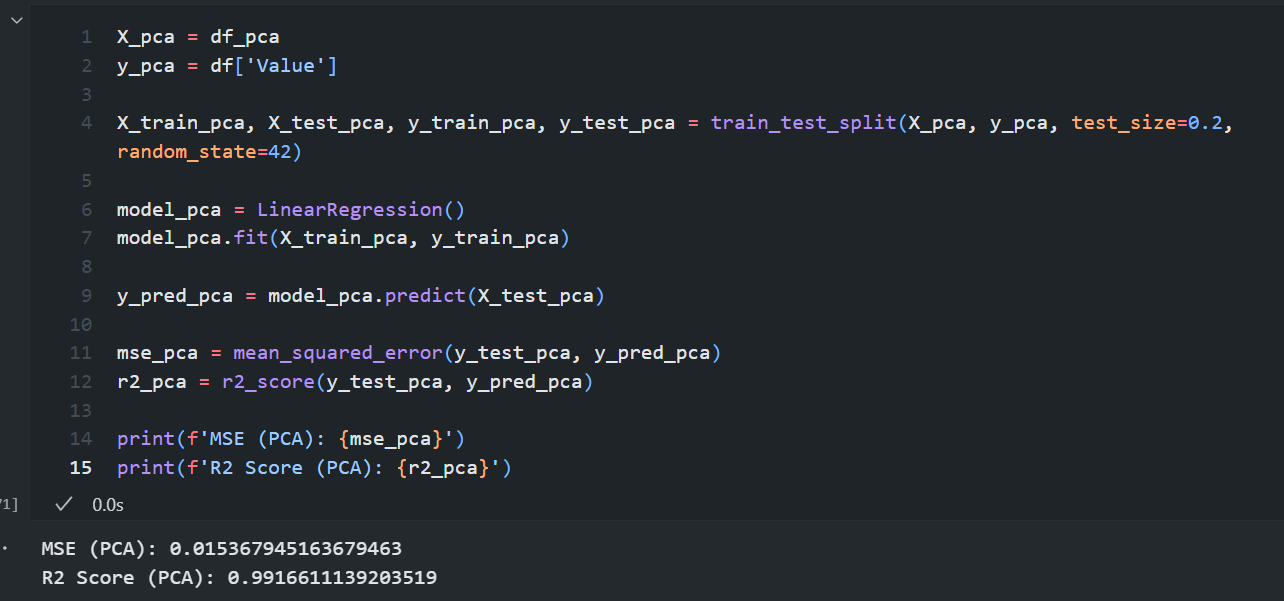
Then I tried Ridge and Lasso regression. Ridge performed the best and outperformed Linear and Lasso, so I’ll stick with Ridge for now until a simpler model comes along.
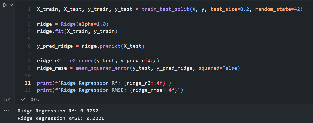
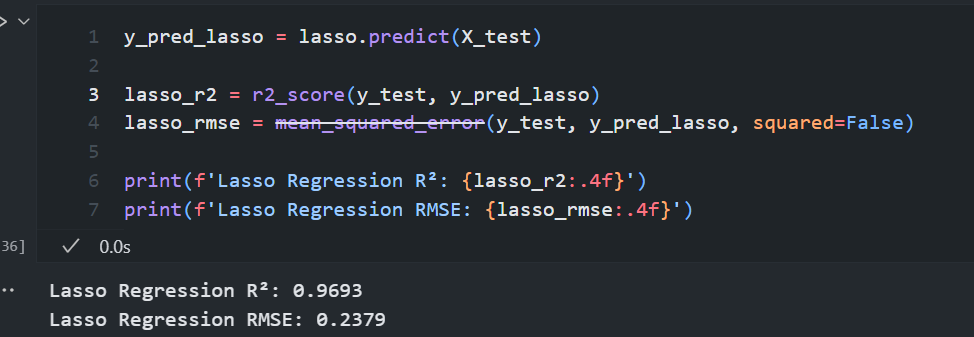
Next up was Decision Tree Regressor. Applied it, and without hyperparameter tuning, I got around a 0.98 R2 score. I know Decision Trees are prone to overfitting, so I visualized, but couldn’t predict by myself. Decided to try hyperparameter tuning, but the results weren’t drastically different.
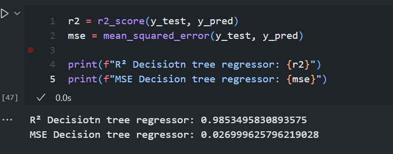
At this point, the Decision Tree is the best model for the project. Let's see what’s coming next. Good luck, city. 𝐒𝐡𝐮𝐯𝐚𝐫𝐚𝐭𝐫𝐢 🌙
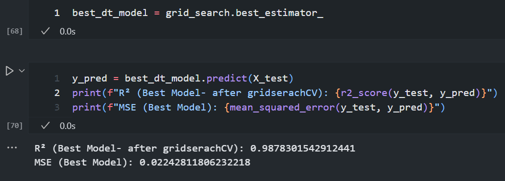
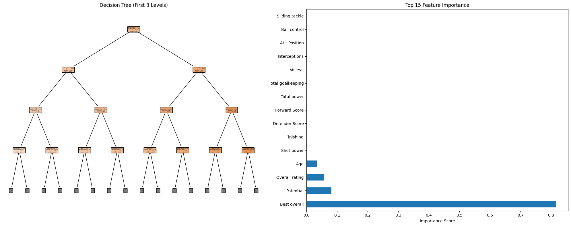
Did i just wasted 2 hours?? 😅😅
Day 61: Project @ Football Players Market Value Prediction -Had to hit reset from Feature Engineering
Just 20 minutes ago, i realized i’ve been making a huge mistake since day 4 with feature engineering. i found out today that as a beginner, it’s easy to mess up, but it's all part of the learning process. the mistkae was thinking about how to transform features back for deployment without realizing that features like overall rating, best oiverall, and potential are actually super correlated with market value. i was happy with the 99% accuracy, but i didn’t see the problem until now. i knew about overfitting can cause it and tried to fix it, but i never thought about visualizing feature importance and how it can affect the model.
So, iwas almost done with the project and deployed it to my local server using streamlit. feeling soooo dumb at the moment. the day before yesterday, i tested it with real players like KDB, Lamine Yamal, and Oblak, and 𝐭𝐡𝐞 𝐩𝐫𝐞𝐝𝐢𝐜𝐭𝐢𝐨𝐧𝐬 𝐥𝐨𝐨𝐤𝐞𝐝 𝐠𝐨𝐨𝐝. 𝐰𝐡𝐲?? 𝐛𝐞𝐜𝐚𝐮𝐬𝐞 𝐢𝐭 𝐭𝐨𝐭𝐚𝐥𝐥𝐲 𝐫𝐞𝐥𝐲𝐢𝐧𝐠 𝐨𝐧 𝐣𝐮𝐬𝐭 𝐭𝐡𝐫𝐞𝐞 𝐢𝐧𝐩𝐮𝐭𝐬 𝐁𝐞𝐬𝐭 𝐎𝐯𝐞𝐫𝐚𝐥𝐥, 𝐎𝐯𝐞𝐫𝐚𝐥𝐥 𝐑𝐚𝐭𝐢𝐧𝐠, 𝐚𝐧𝐝 𝐏𝐨𝐭𝐞𝐧𝐭𝐢𝐚𝐥. 𝐲𝐨𝐮 𝐜𝐚𝐧 𝐞𝐯𝐞𝐧 𝐩𝐫𝐞𝐝𝐢𝐜𝐭 𝐰𝐡𝐨𝐥𝐞 𝐭𝐡𝐢𝐧𝐠𝐬 𝐰𝐢𝐭𝐡 𝐣𝐮𝐬𝐭 𝐭𝐡𝐞𝐬𝐞 𝐢𝐧𝐩𝐮𝐭𝐬. The impact of other features is literally minimal. now, i have to rebuild the model from scratch again with better feature engineering.
Even after this dumbest mistake, total wasted grinding, wasted time, wasted energy---for the first time in my learning journey, it feels like now i'm actually learning something.
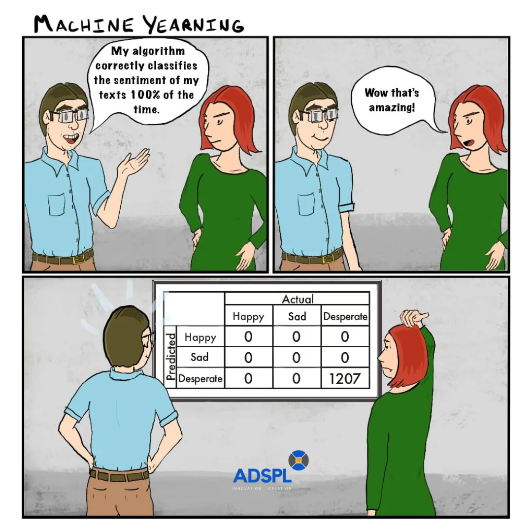
Day 62: Project @ Football Players Market Value Prediction - Finalizing Project and Deploying it
Finally, i’m able to go live with my first end-to-end ml project! 🎉 you can check it out here: https://paudelsamir.streamlit.app/
- Today was all about polishing things i messed up, after some solid feature engineering, i was able to hit 85% accuracy, pretty solid start. then, i played around a hour with hyperparameter tuning, which bumped it up to 89%.
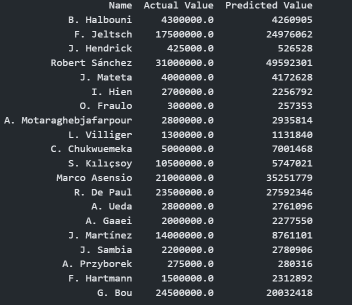
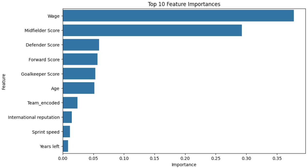
but the real magic happened when i tried ensemble learning techniques. after a bit of back and forth, gradient boosting took me all the way to 94% accuracy. and will be using the same algorithm for deployment too.
And with that, after 10 days of nonstop grinding, i’m officially closing this project. it’s been a fun ride, full of learning and surprises !!
𝐆𝐢𝐭𝐇𝐮𝐛 𝐑𝐞𝐩𝐨 For the Project: https://github.com/paudelsamir/ML-Based-Football-Players-Market-Value-Prediction
Day 63: Content-Based Movie Recommender System - Preprocessing
Today, I focused on the preprocessing phase of building a content-based movie recommender system. I created a tags feature by combining key keywords from columns like genres, descriptions, top 3 cast members, and crew, especially the director. This step was crucial to ensure that the recommendation engine has a rich set of features to work with.
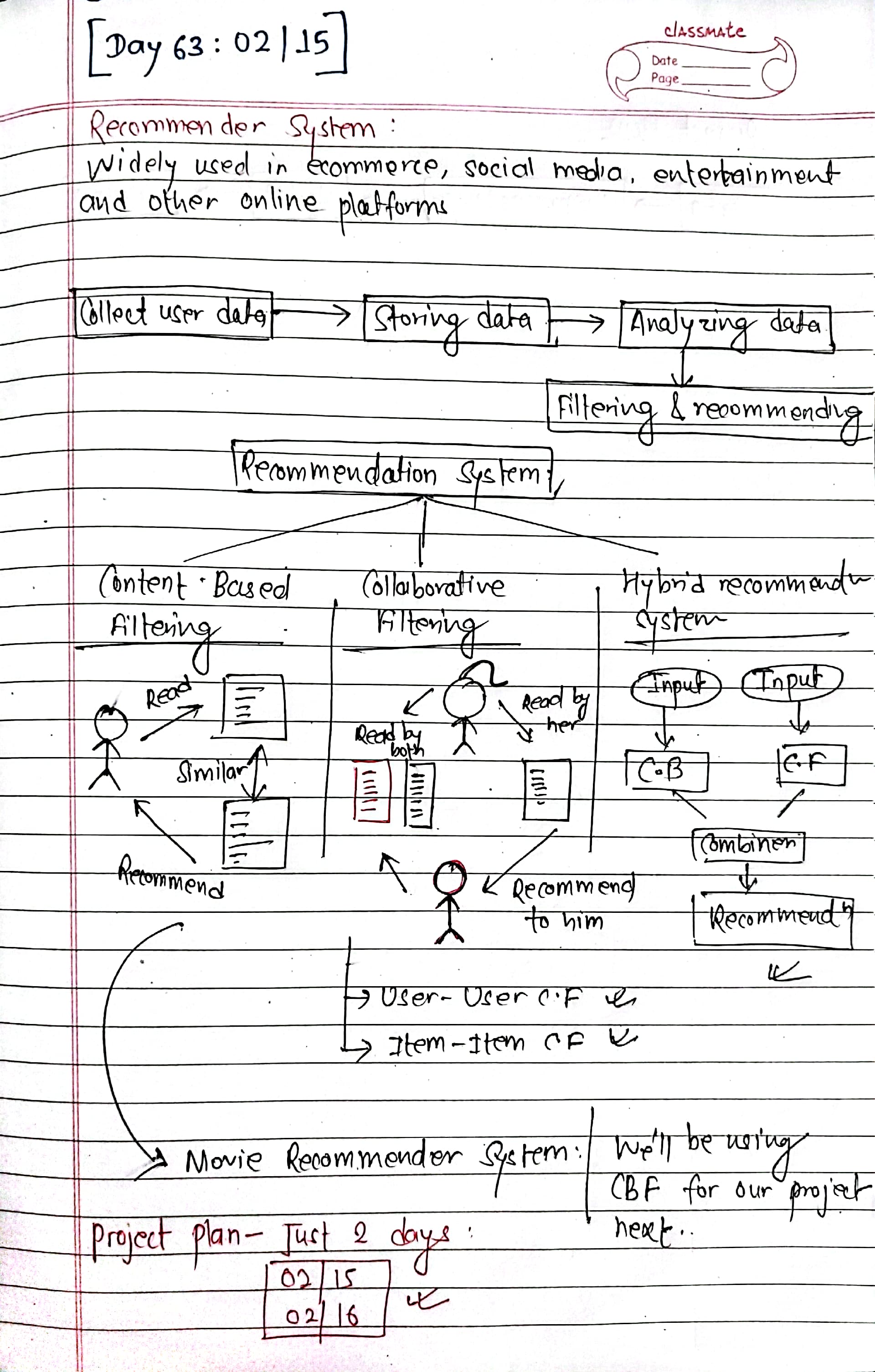
Day 64: Content-Based Movie Recommender System - Building and Deployment
Today, I built the recommendation engine based on movie content similarity using vectorization (bag of words). I also deployed it with Streamlit, so now you can input a movie name and get the top 5 similar movies based on the similarity matrix. Additionally, I integrated an API to pull movie posters in real-time from the website TMDB!
𝐂𝐡𝐞𝐜𝐤 𝐨𝐮𝐭 𝐡𝐞 𝐥𝐢𝐯𝐞 𝐝𝐞𝐦𝐨 𝐡𝐞𝐫𝐞: https://lnkd.in/d7R3Wsnk
Day 65: Diving into Deep Learning
Explored deep learning concepts, including its significance, how it differs from machine learning, and whether it will replace ML. Covered key architectures like Feedforward Neural Networks (FNNs), Convolutional Neural Networks (CNNs) for image processing, Recurrent Neural Networks (RNNs) for sequential data, Autoencoders for feature learning, and Generative Adversarial Networks (GANs) for data generation.
Notes from the day:
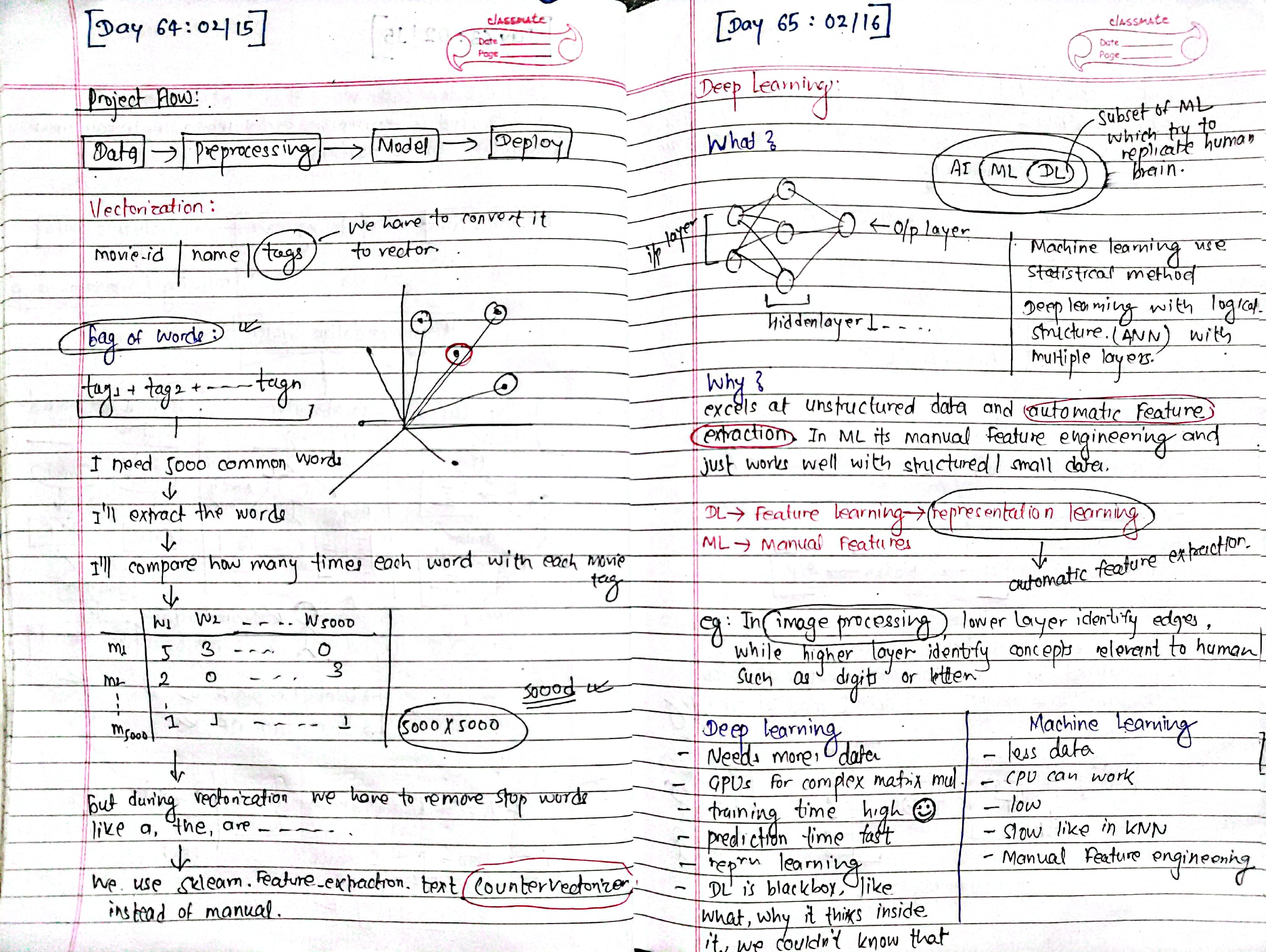
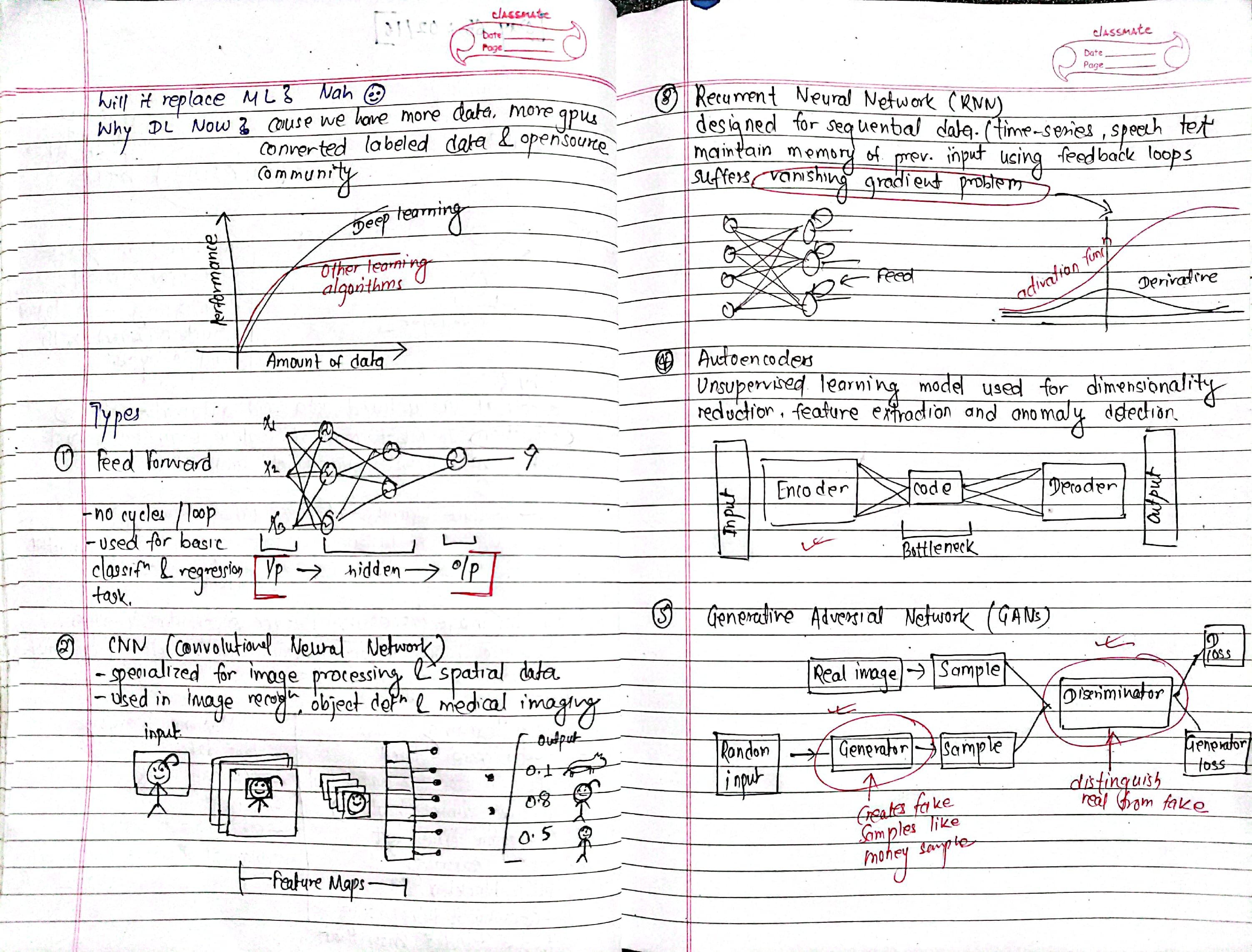
- Types of Neural network:
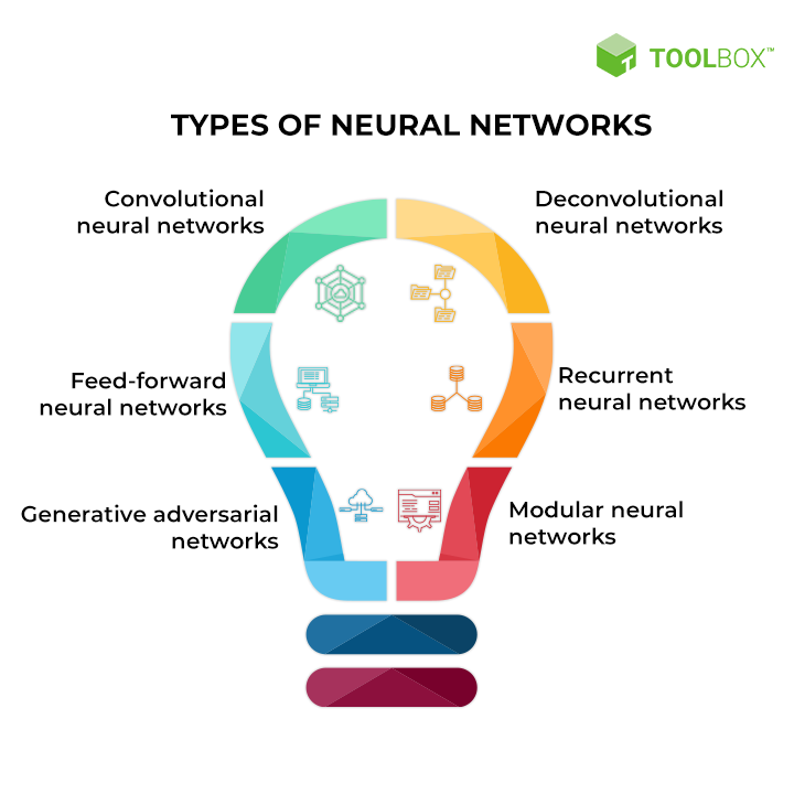
Day 66: Perceptrons
Today, I dived into the concept of perceptrons, which are the building blocks of neural networks. I explored the perceptron algorithm, its working mechanism, and how it can be used for binary classification tasks. A supervised learning algorithm used for binary classifiers.
-
Steps in Prceptron Algorithm:
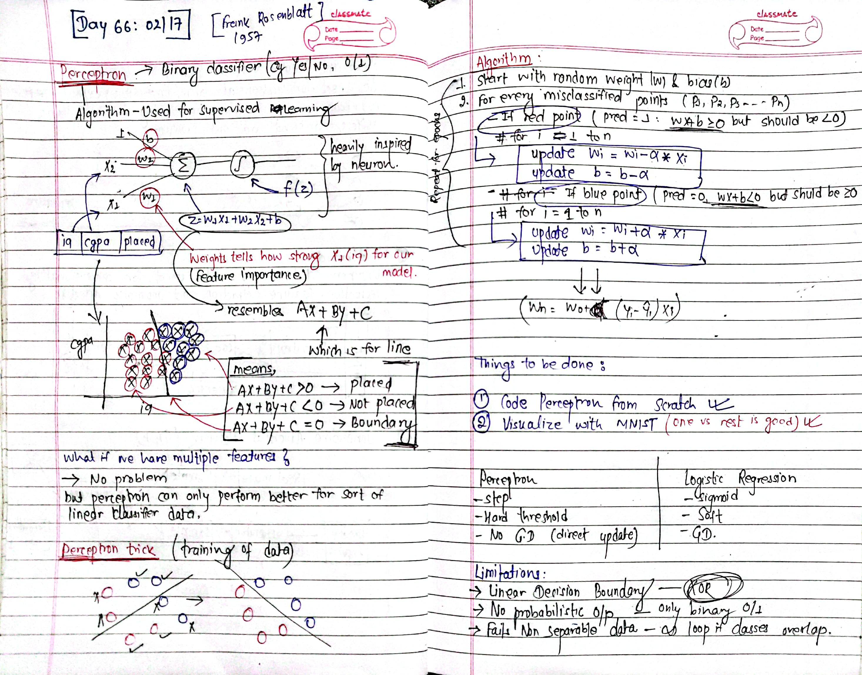
-
Perceptron from Scratch:
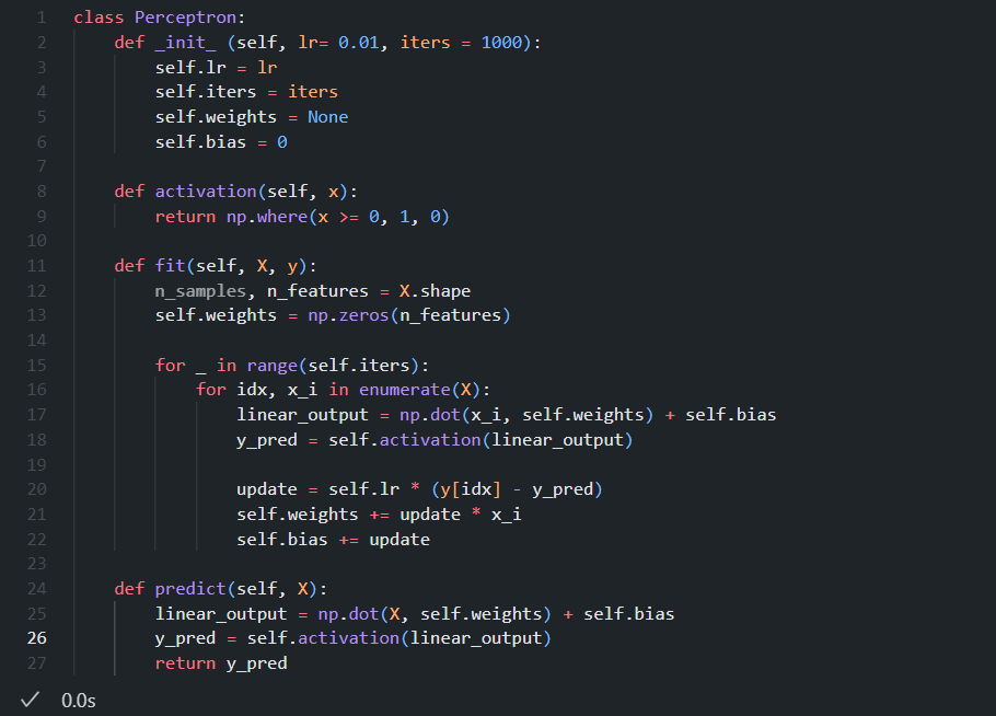
Visuals:
- Training Data:
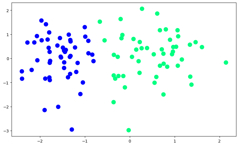
- Perceptron Training:
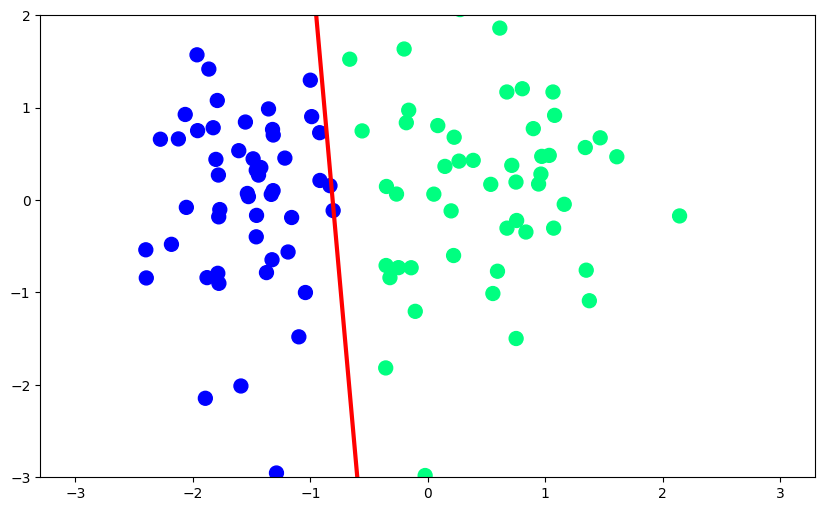
I explored the fundamentals of MLOps with this paper: Machine Learning Operations (MLOps): Overview, Definition, and Architecture : https://arxiv.org/pdf/2205.02302
Day 67: Perceptron Loss Function and Gradient Descent
Today, I explored the Perceptron Loss Function, which helps adjust weights when misclassification occurs, ensuring better decision boundaries. I learned how the perceptron updates its weights using the weight update rule and how Gradient Descent optimizes the loss function by iteratively moving in the direction of the negative gradient.
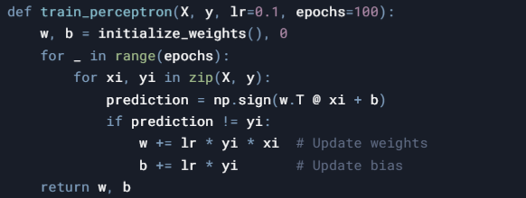
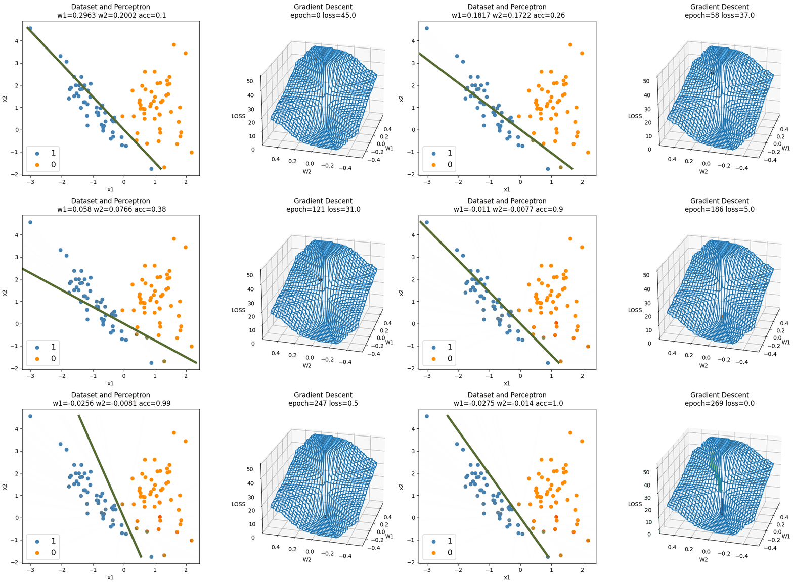
Notes:
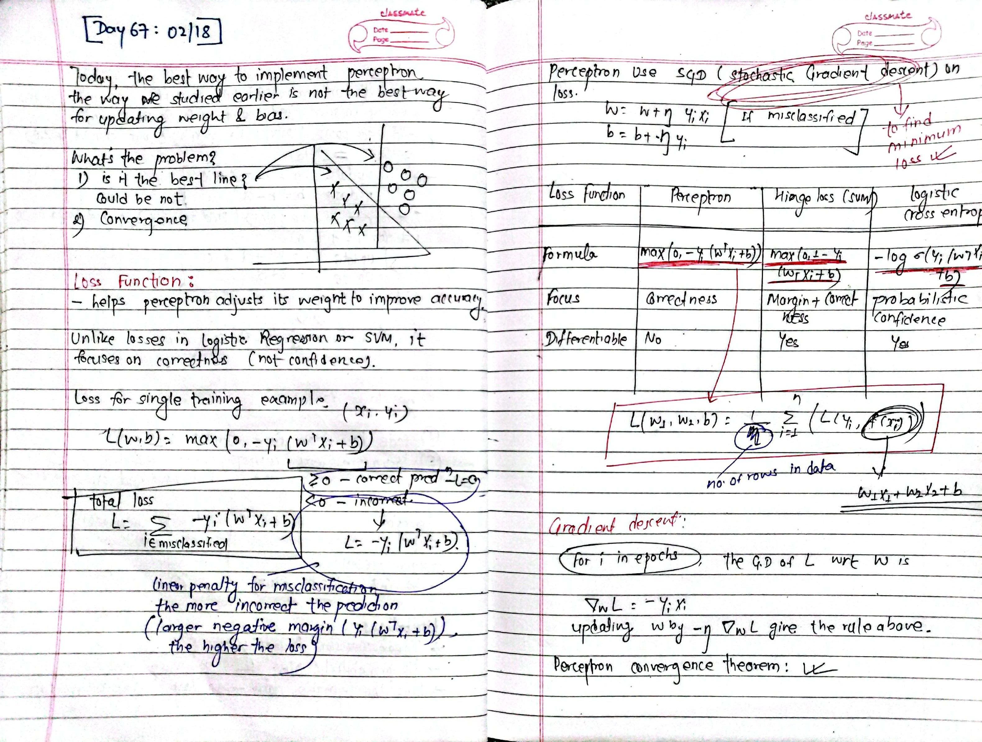
Day 68: Multilayer Perceptron
The problem with Perceptrons lies in their limitation to learn complex patterns and functions, especially those that are not linearly separable. A Perceptron is a single-layer neural network with binary outputs, and it can only solve problems where the data points are linearly separable. If the data is not linearly separable, a Perceptron cannot converge and find a solution.
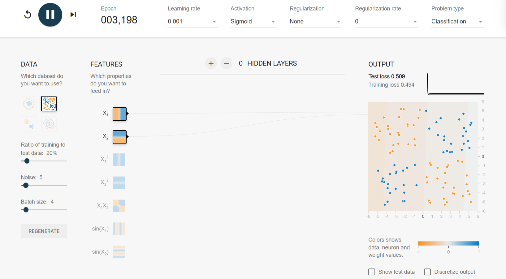
So the solution is Multilayer Perceptron:
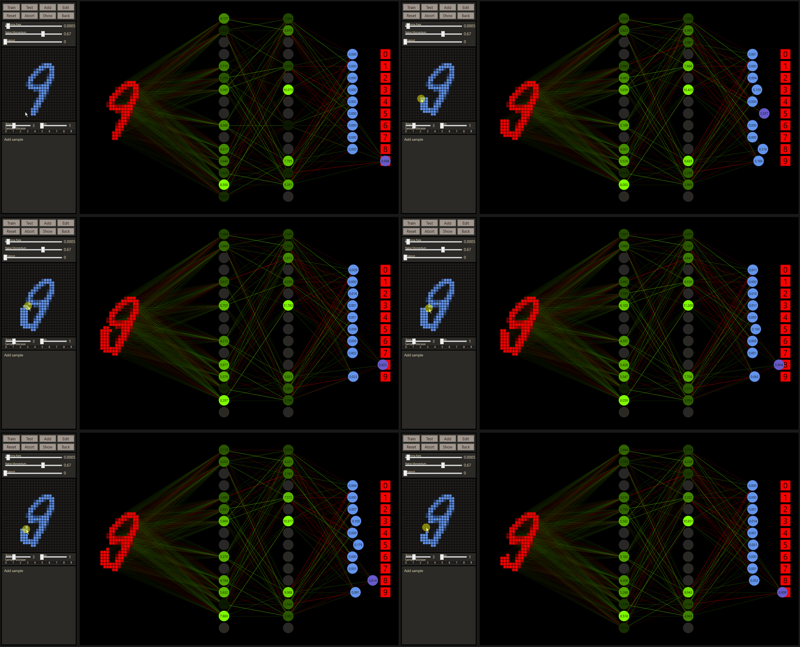
There's a website named: https://playground.tensorflow.org/
I practiced different optimizations there some of them are,
- Adding nodes to hidden layer
- Adding nodes to input layer
- Adding nodes to output layer (for multicalss)
- Adding nuber of hidden layer
The conclusion is you can classify any type of problem within regression and classifcion by optimizing those nodes and others like activation and regularization.
Batch and Gradient Descent:
number of samples processed before updating model weights
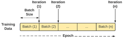
- SGD (batch size = 1) → updates after each individual sample (one row at a time). noisy but good for escaping local minima.
- Mini-batch gradient descent (batch size = 16, 32, 64, etc.) → updates after a small group of samples (e.g., rows 1-100). balances speed and stability.
- Full-batch gradient descent (batch size = all samples) → updates after seeing the entire dataset. very stable but slow and memory-heavy.
each batch in mini-batch or full-batch contains multiple rows, and the loss is computed over those samples before updating weights.
so in SGD, you're updating weights after every single row (which makes it very random and noisy). in mini-batch, you take a chunk of rows, calculate gradients over that group, then update weights. in full-batch, you process all the rows at once and then update.
Notes:
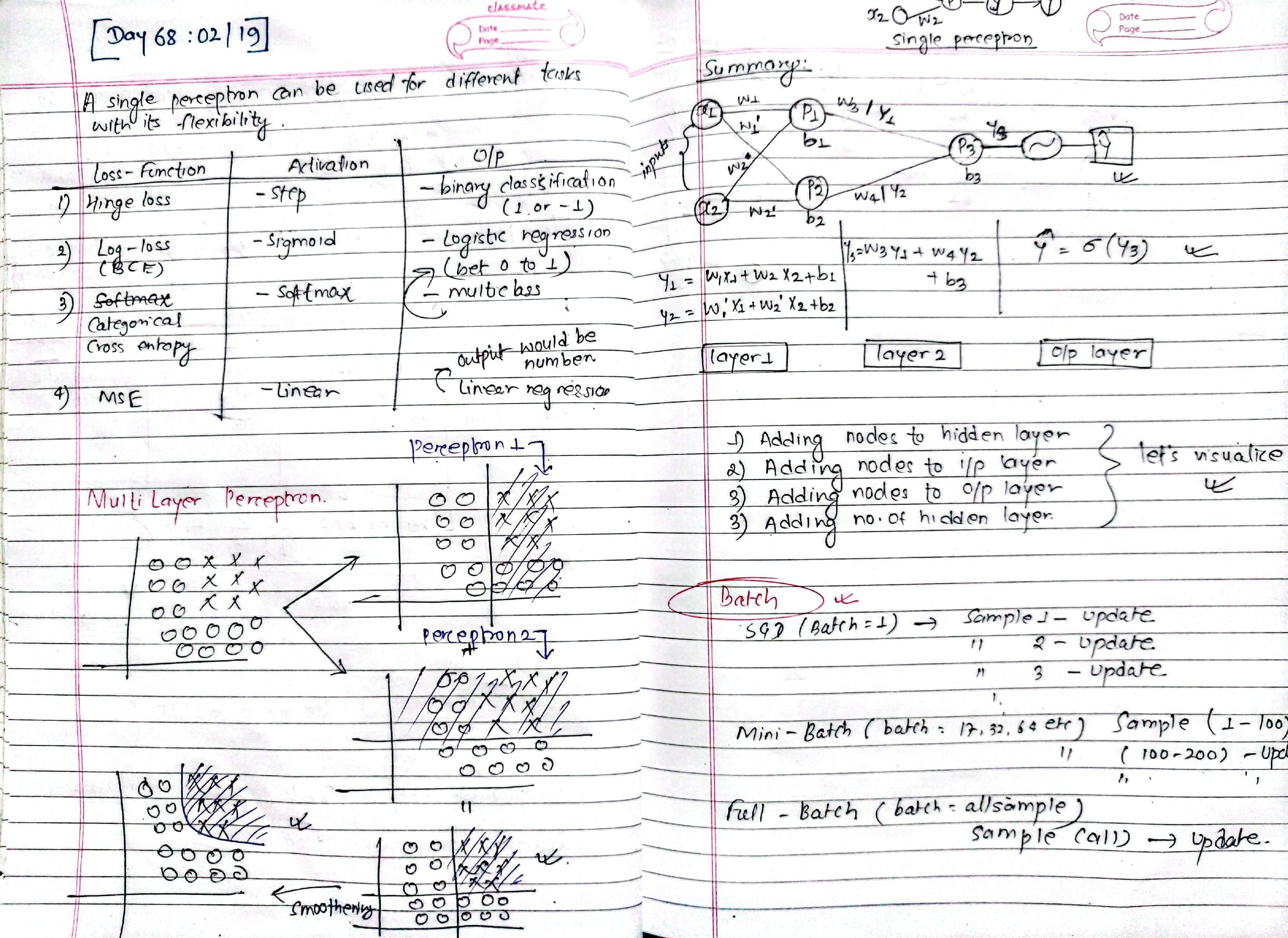
Day 69: MLP notation, Forward Propagation
today, i deepened my understanding of multi-layer perceptrons (MLPs), including their formal notation and the calculation of weights and biases for each layer. i also explored forward propagation and practiced matrix multiplication by manually constructing and multiplying matrices to intuitively follow the perceptron’s computations.
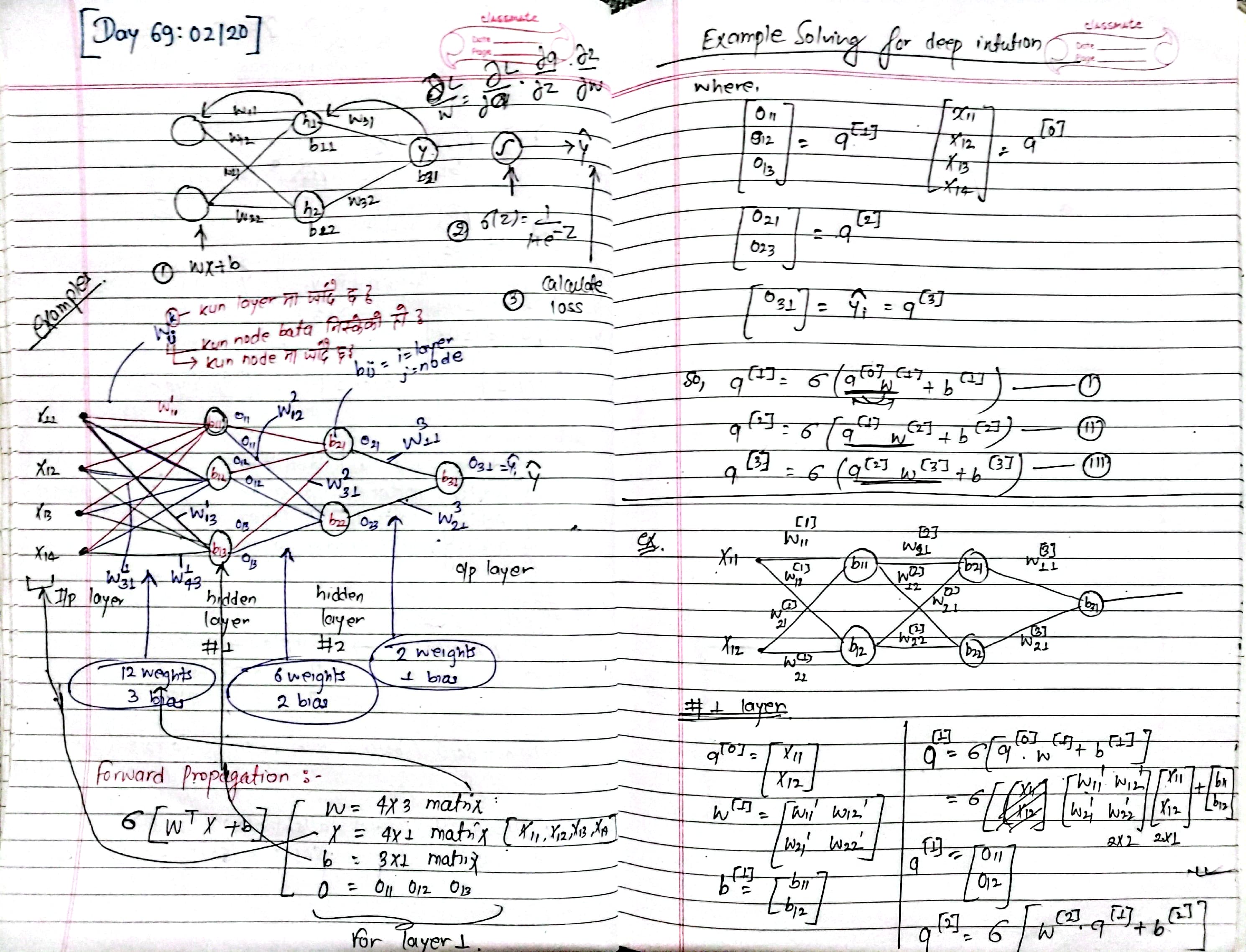
additionally, i studied MLP training with pytorch from the book deep learning with python by françois chollet.
additionally, i explored Image processing with datacamp, here's image representation of what i learned today
Day 70: Loss Functions for Deep Learning
-
Regression:
- MSE : squares errors, punishes big mistakes more.
- MAE : takes absolute difference, treats all errors equally.
- Huber Loss: mix of mse & mae, good for outliers.
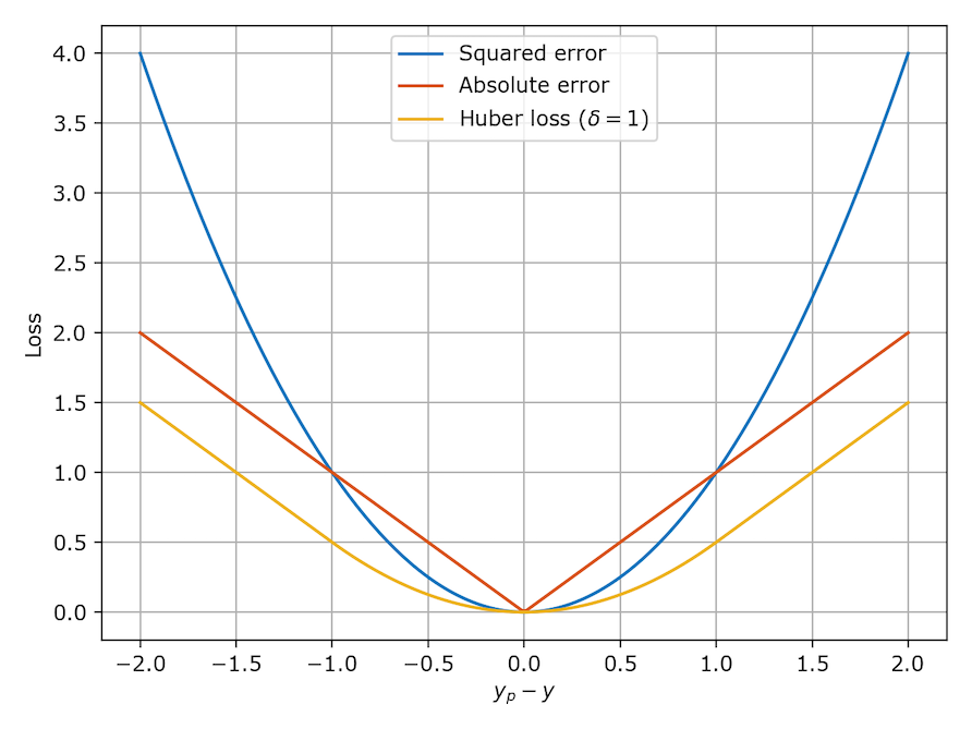
-
Classificaiton:
- Binary cross entropy : for yes/no classification (spam or not spam).
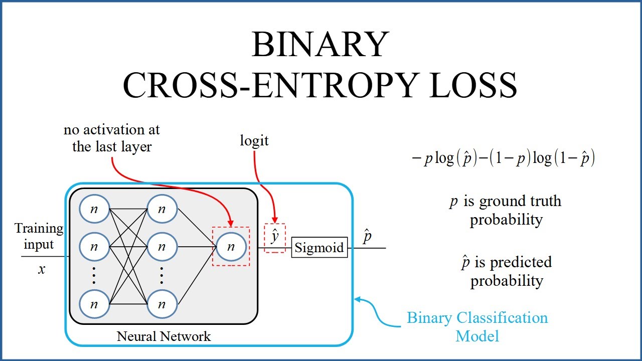
- Categorical Cross entropy : for multiple classes (yes/no/ maybe).
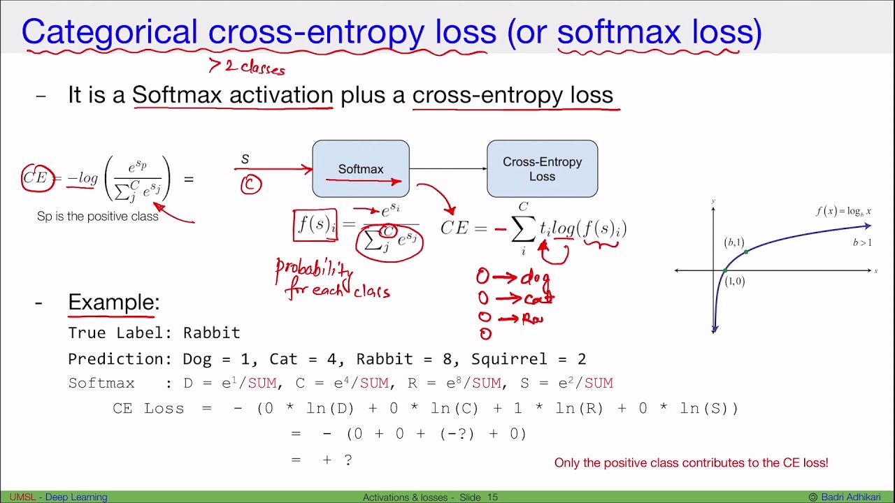
- Sparse Categorical cross entropy - same as categorical but works with integer labels.
- Hinge Loss: used in SVMs, pushes correct class far from the wrong ones.
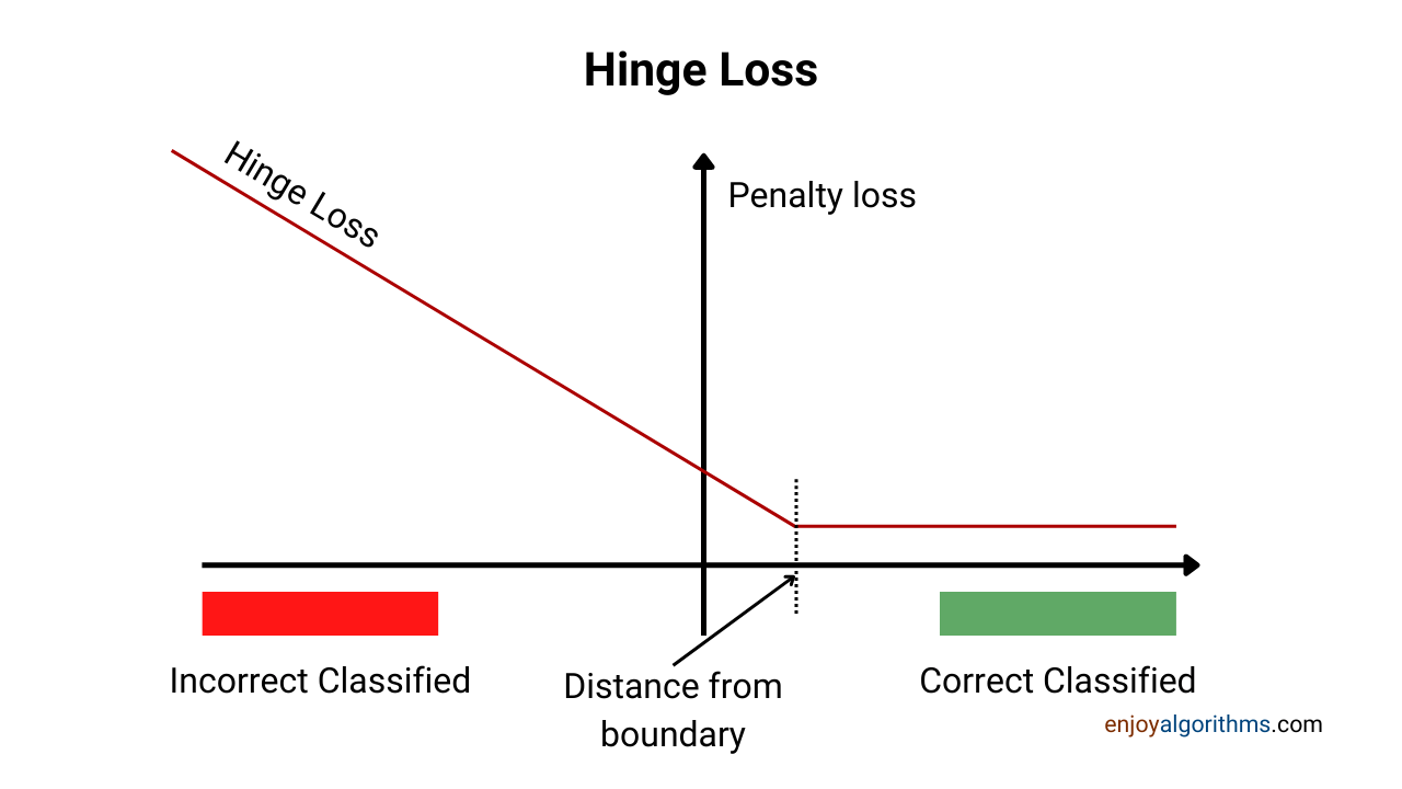
- Binary cross entropy : for yes/no classification (spam or not spam).
-
Autoencoders / VAE loss:
- KL divergence
-
GANs:
- Discriminator loss : helps the discriminator tell real from fake.
- Minmax Loss : generator tries to fool discriminator by minimizing its best-case performance.
-
Object Detection and segmentation loss:
- interseciton over union loss
- smoooth l1 loss
- dice loss
-
Reinforcement loss:
- policy gradient - rewards good actions.
- Q-Learning loss : teaches agent to choose best long-term rewards.
- proximal policy optimization
-
Custom losss function:
- Perceptrual loss
- combined loss functions: mix of different losses for better results (e.g., cross-entropy + dice loss).
Notes:
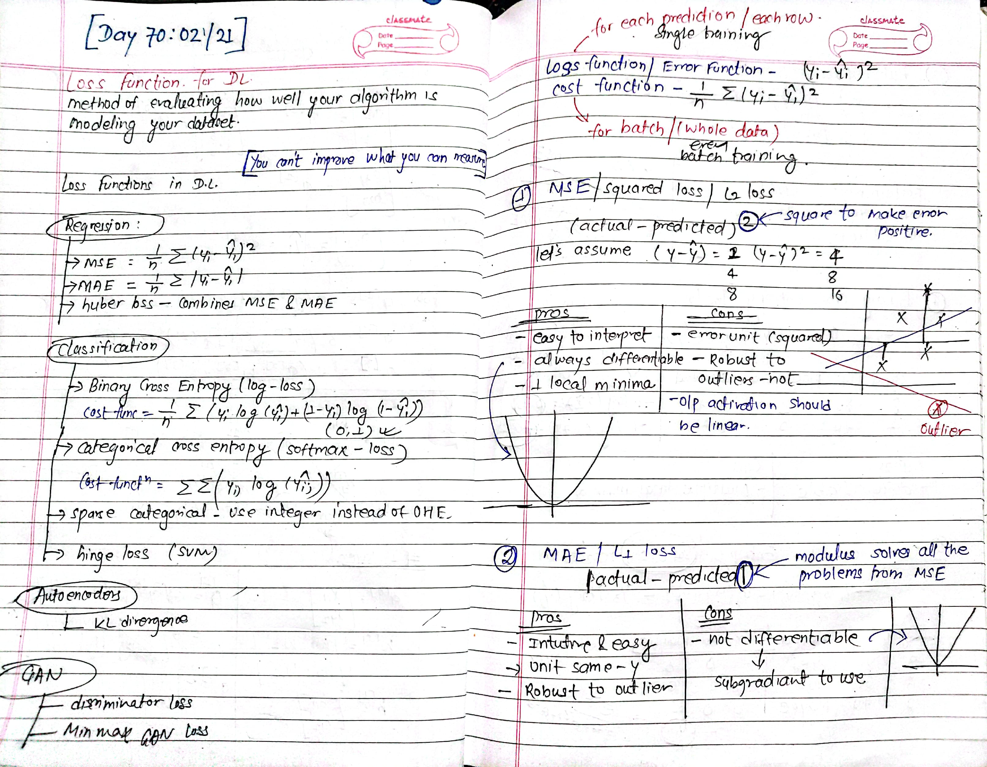
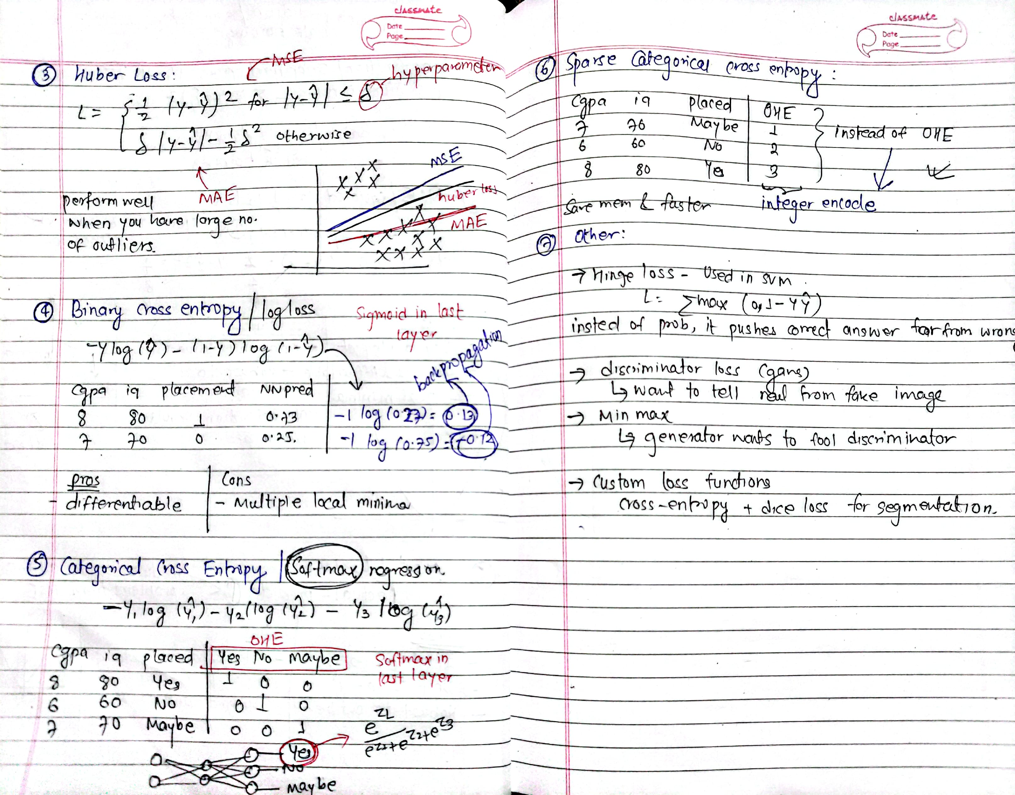
Day 71: Deep Diving Backpropagation
I already explored backpropagation in andrew ng’s ml specialization course, but that was more of a surface level explanation just the mechanics of how it works.
Today, i’m diving deep. like, REALLY deep. i want an intuitive, mathematical understanding of backpropagation, not just the algorithmic steps. all my tracing and derivations are going into my handwritten notes. this is for intutive approach to understand Regression part.
Notes:
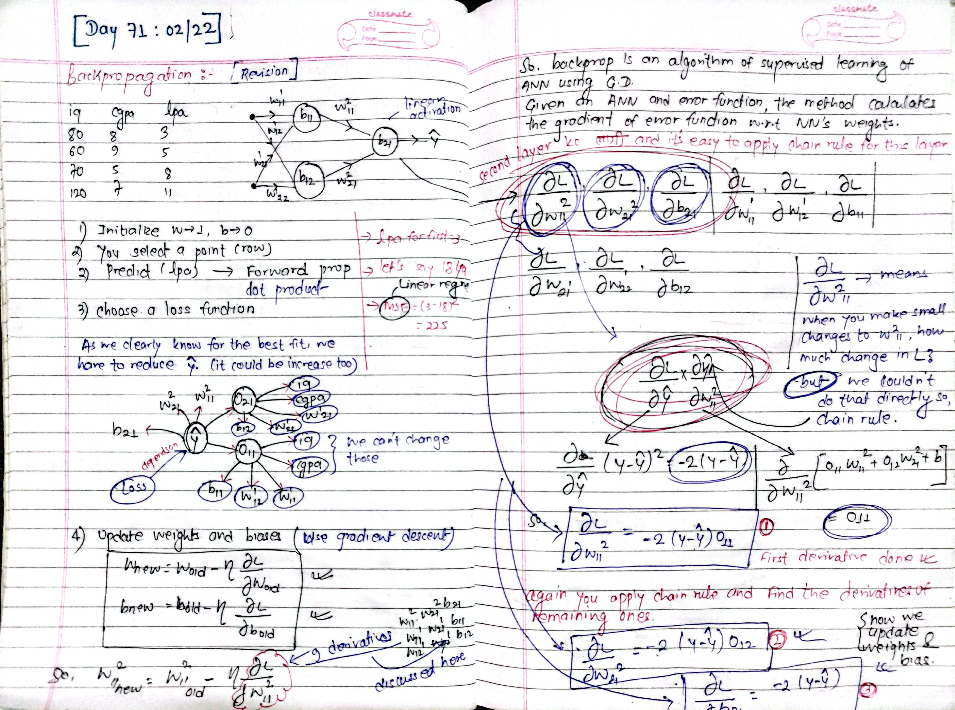
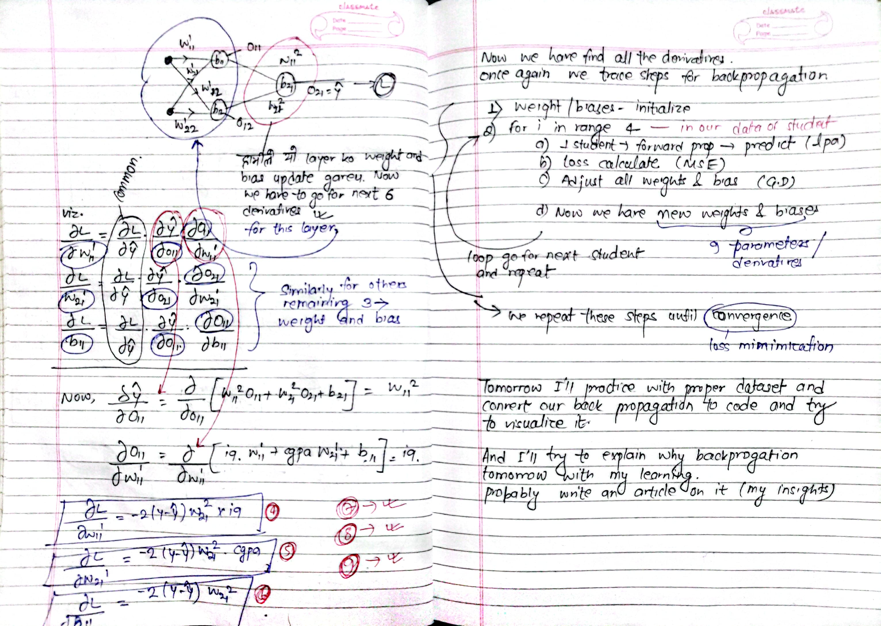
Tomorrow, i’ll probably implement backprop from scratch, test it on a proper dataset, and try to visualize what’s actually happening. the key question: how?
Also, i might challenge myself to explain why backprop works in my own words. maybe even turn it into an article.
Day 72: Implementing backpropagation for regression
Today was all about applying what i learned yesterday to code and visualizing backpropagation.
first, i created a toy dataset that looks like this:
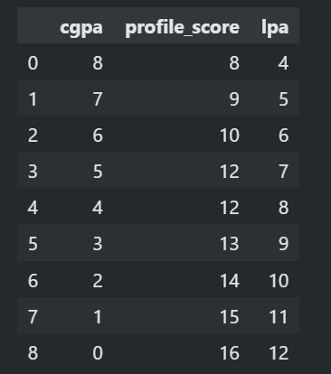
Then, i wrote functions to implement backpropagation from scratch. after running the training loop, here’s what the final parameters looked like—no keras, no tensorflow, just raw python:
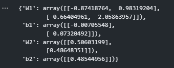
all the code is in my notebook:
Notebook: Backpropagation Regression
I also tried using keras' sequential api to train the same model. after around 700 epochs, the error dropped significantly.
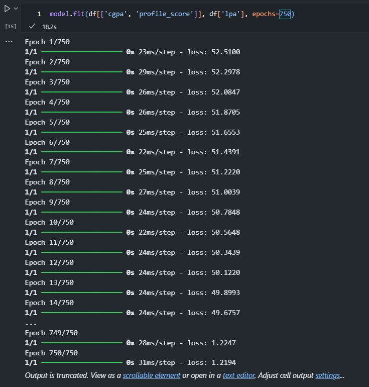
final weights with keras:
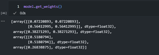
PS: intentionally chose a confusing dataset to mess with my own head.
Day 73: Implementing Backpropagation for Classification
i already implemented backprop for regression, both handwritten and in code. today, i'm tweaking it for classification.
few things to change:
- loss function is binary cross-entropy instead of MSE
- activation function is sigmoid instead of linear
but the backprop algo stays the same. all derivatives are now based on the new log function. since i already get the intuition, i'm skipping the math and just coding it.
Notebook: implementation backprop classification
sample data looks like this:
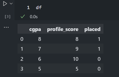
final parameters after training:
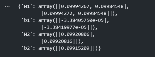
function to update parameters:
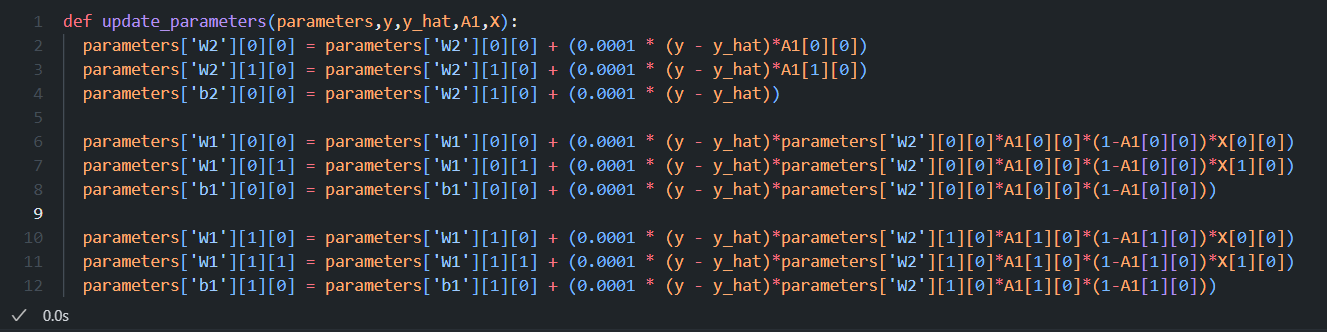
at last, i tried implementing the same using tensorflow to see how it compares to my scratch implementation:
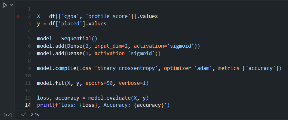
Day 74: Revising old days, Memoization
Today, i revised concept of gradient and derivatives, focusing on how subtracting the gradient term is helping minimize loss. gradient relies on derivatives to find the optimal weights, and the learning rate controls the step size too high can cause overshooting, while too low leads to slow convergence. another key takeaway was memoization, a technique to store previously computed values to optimize calculations. in neural networks, repeated derivative computations can slow down training, and memoization helps speed things up by avoiding redundant calculations. this approach is widely used in dynamic programming and can improve efficiency in deep learning models.
Notes:
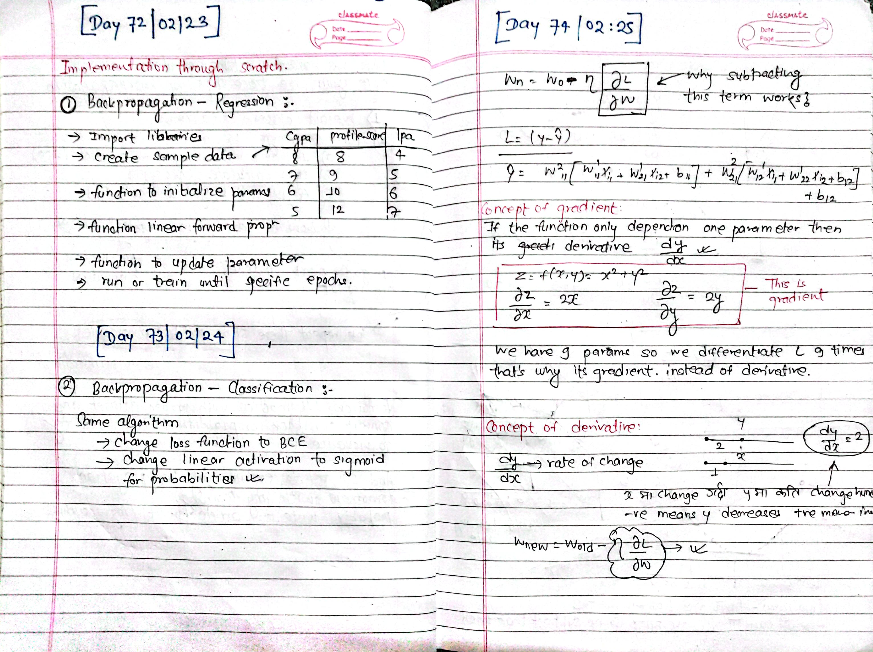
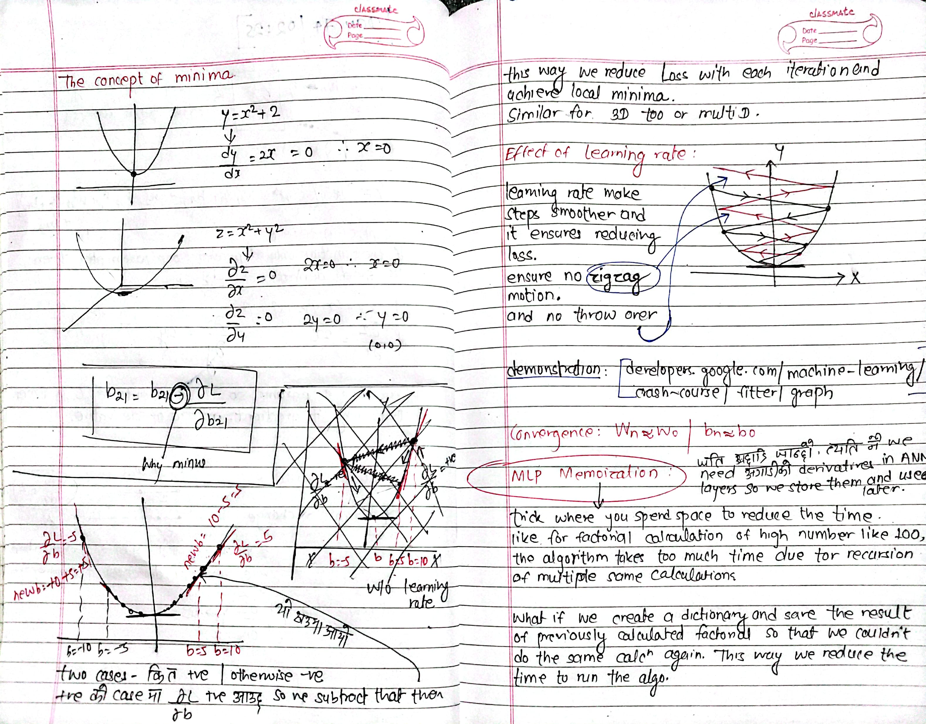
Day 75: Vanishing Gradient, Exploding Gradient
Today i first revised Gradient descent in NN:
-
Batch : faster to complete epochs ( batch size = all)
-
Stochastic : faster to converge ( batch size = 1)
-
Mini- Batch : mostly suitable ( batch size around center)
-
vanishing gradient: when gradients become too small, causing early layers to learn very slowly or not at all. example: in deep networks using sigmoid activation, earlier layers stop updating because gradients shrink to near zero.
-
exploding gradient: when gradients become too large, leading to unstable updates and divergence. example: in rnn training, weights keep multiplying large gradients, causing values to explode to infinity.
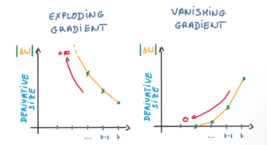
How to Handle VGD problem:
- use better activation functions – replace sigmoid/tanh with relu, leaky relu, or elu.
Using Sigmoid:
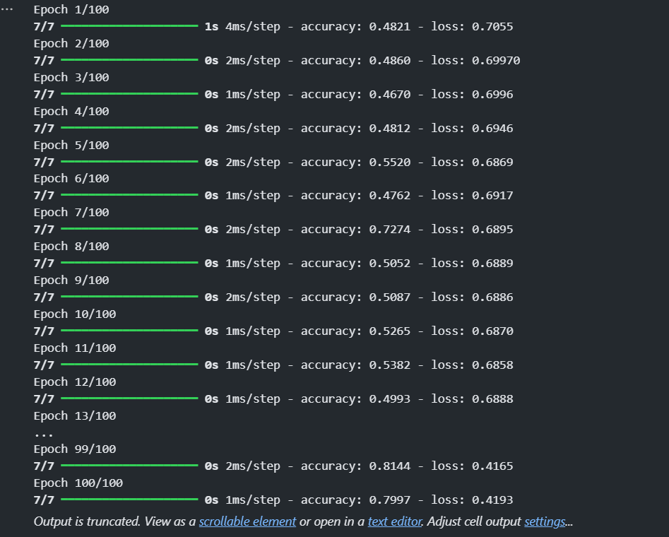 Using ReLU:
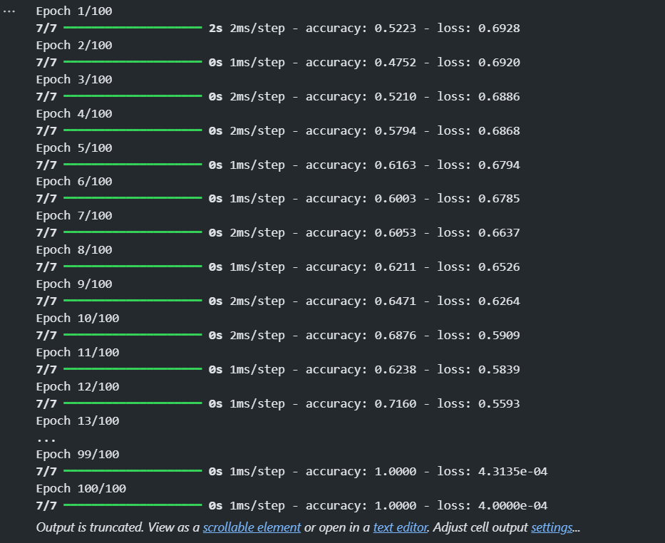 This is the final weights comparision:
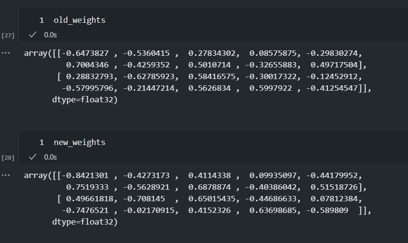
- use proper weight initialization – xavier/glorot for sigmoid/tanh, he initialization for relu.
- batch normalization – normalizes activations to maintain stable gradients.
- residual connections (skip connections) – used in resnets to allow gradients to flow easily.
- gradient clipping – caps gradients to prevent them from becoming too small.
Day 76: Implementing artificial neural networks (ann) for different datasets
- Experimented with ann on two datasets: mnist for handwritten digit classification and a gre dataset for graduate admission prediction. the goal was to train models and analyze performance across different domains.
Notebook: GRE prediction
Notebook: MNIST Classification
- trained an ann on mnist to classify handwritten digits (0-9) using a sequential model with dense layers. training ran for 30 epochs with promising results.
- training results (30 epochs):
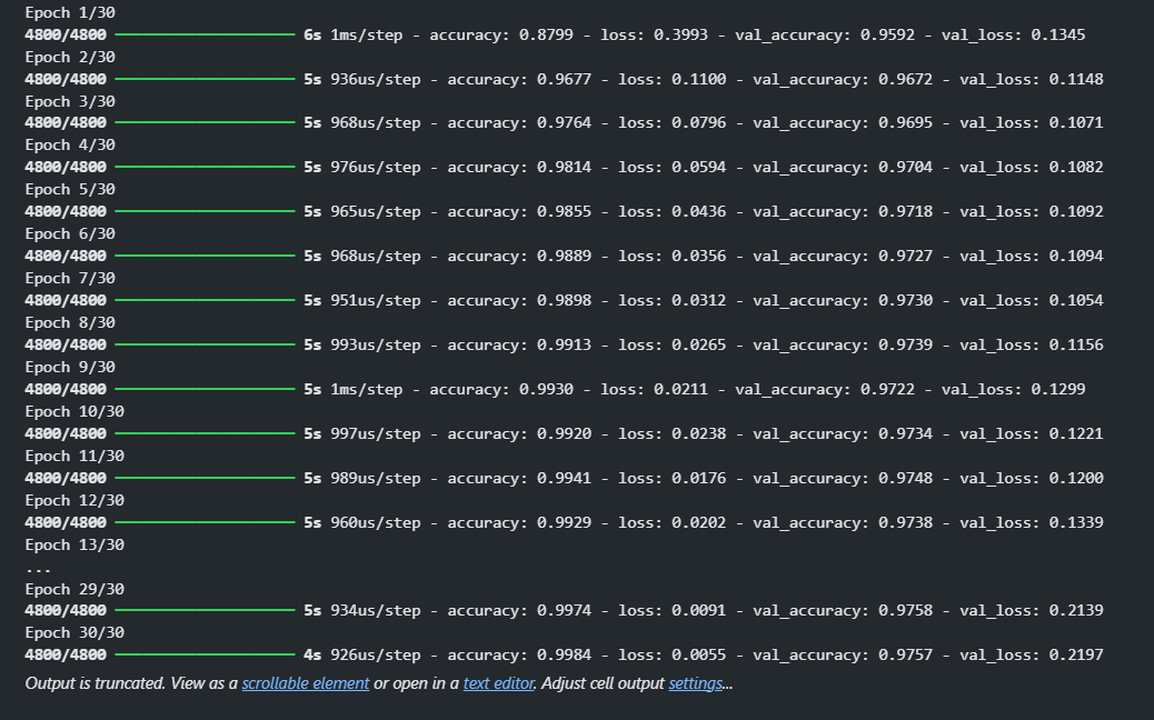
- model summary:
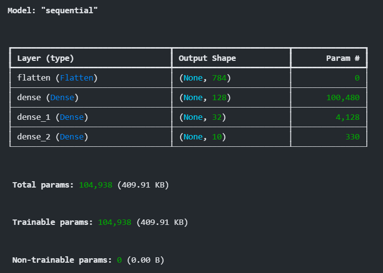
- sample predictions:
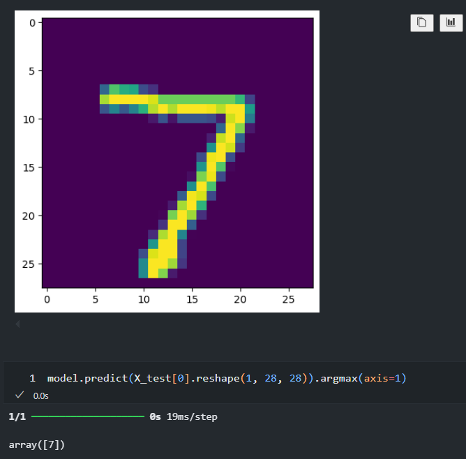
- training results (30 epochs):
- applied ann to predict graduate school admission chances based on gre scores, gpa, and other factors. dataset required preprocessing before feeding into the model. trained for 100 epochs.
- sample dataset:
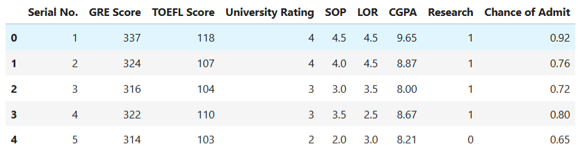
- training results (100 epochs):
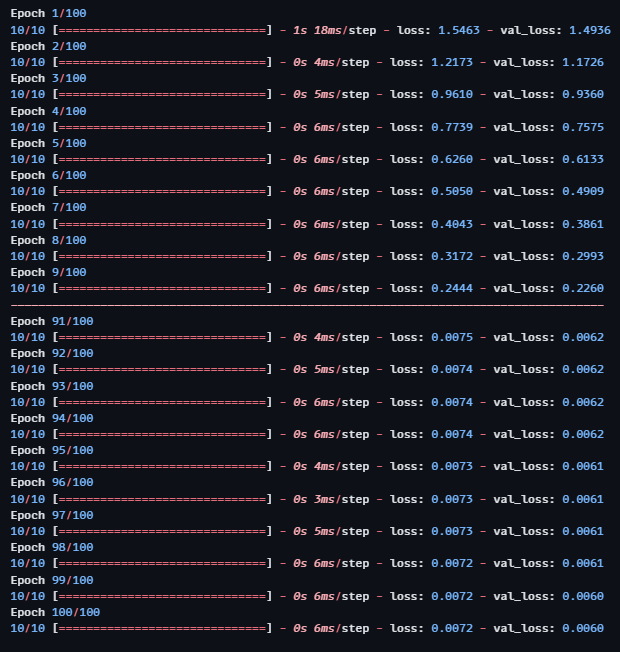
- model summary:
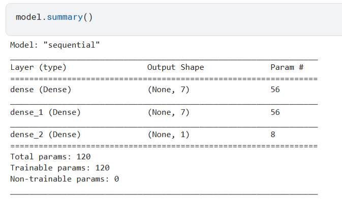
- model accuracy evaluation:
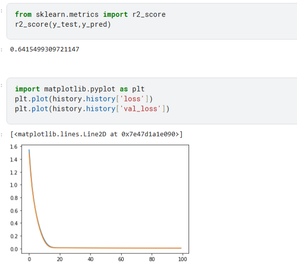
- sample dataset:
next steps: hyperparameter tuning, dropout layers for regularization, and testing on additional datasets.
Day 77: Improving Neural Networks
Notes:
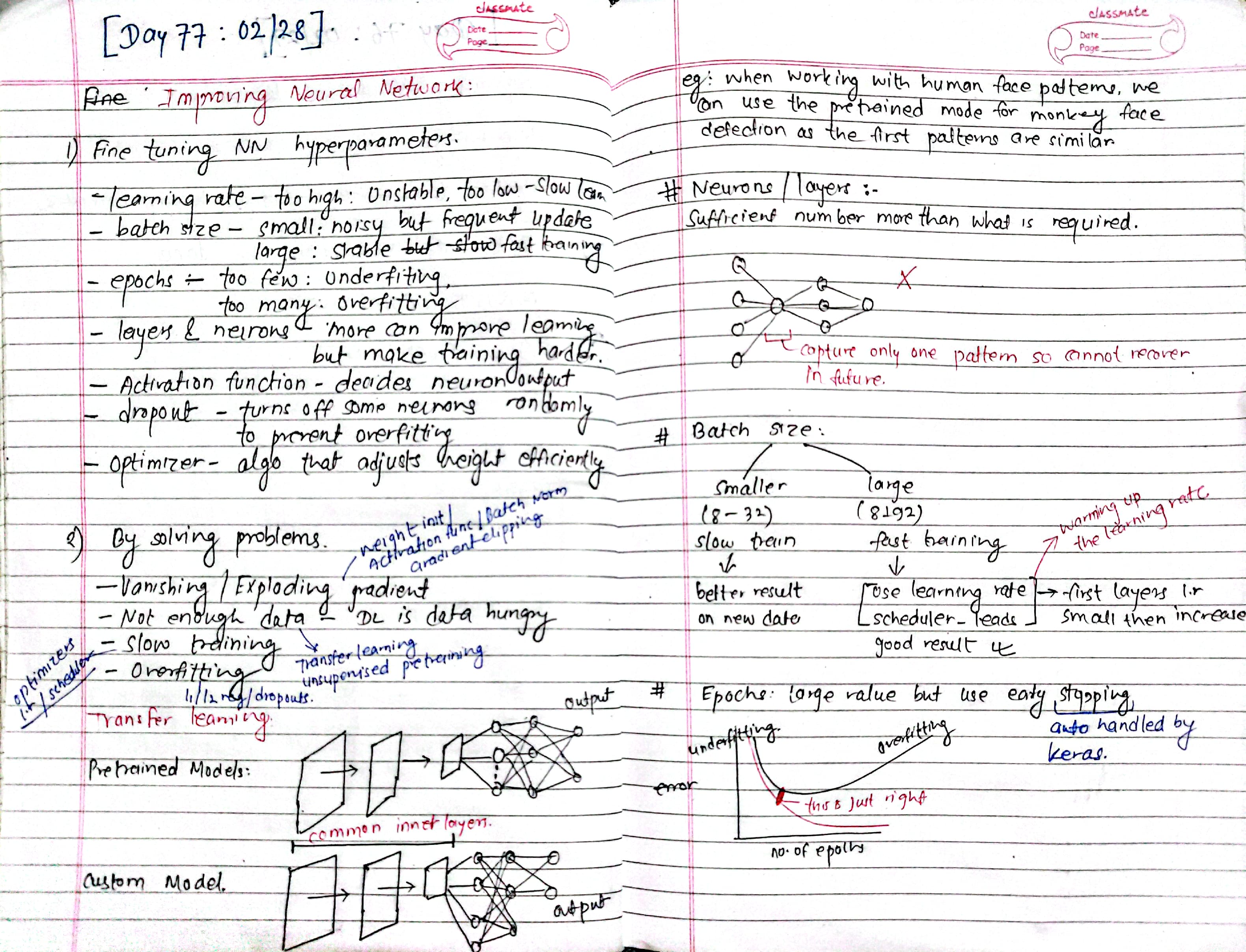
Fine-tuning Neural Network Hyperparameters
Fine-tuning neural network hyperparameters is about adjusting key settings to improve learning
- Learning rate - controls how fast the model updates. Too high = unstable, too low = slow learning.
- Batch size - number of samples processed before an update. Small = noisy but frequent updates, large = stable but slow.
- Epochs - full passes through data. Too few = underfitting, too many = overfitting.
- Layers & neurons - more can improve learning but make training harder.
- Activation function - decides neuron output; common ones are ReLU, sigmoid, tanh.
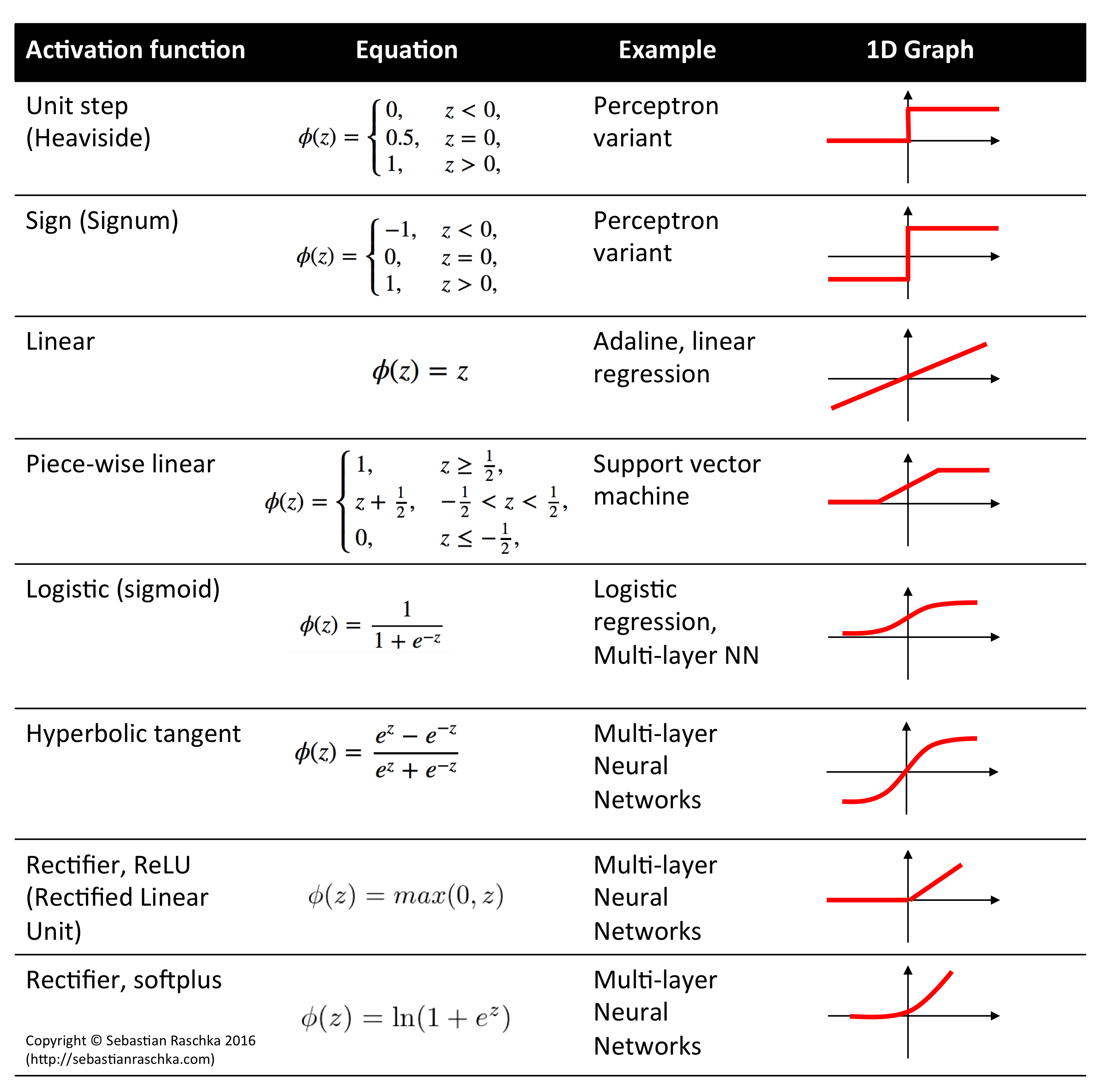
- Dropout - turns off some neurons randomly to prevent overfitting.
- Optimizer - algorithm that adjusts weights efficiently (Adam, SGD, etc.).
Problem Solving Strategies
- Vanishing/exploding gradient – gradients shrink or blow up, stopping learning → use ReLU, batch norm, weight init, or residual connections.
- Not enough data – small datasets cause poor generalization → apply data augmentation, transfer learning, or synthetic data generation.
- Slow training – long training times due to large models or bad optimizers → use mini-batches, better optimizers, mixed precision, and GPUs.
- Overfitting – model memorizes training data but fails on new data → apply dropout, regularization, early stopping, and data augmentation.
- Underfitting – model is too simple and fails to learn patterns → increase complexity, train longer, improve features, and reduce regularization.
- Imbalanced data – one class dominates, leading to biased predictions → use class weighting, oversampling, or synthetic data (SMOTE/GANs).
- Poor generalization – model does well in training but fails on real-world data → ensure diverse data, reduce leakage, use domain adaptation, or adversarial training.
Transfer Learning
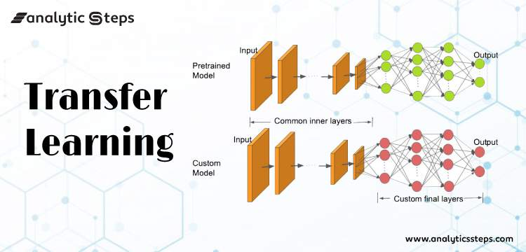
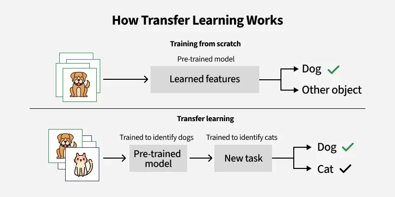
Day 78: Sequence Modeling / RNNs - Just Overview
I just thought ki Before diving deeper into neural network improvement techniques, I should first gain a surface-level understanding of deep learning concepts I'll be tackling in the future as this learning technique is helping me alot. For this purpose, I found an excellent YouTube playlist: MIT 6.S191: Introduction to Deep Learning. There are approximately 10 to 15 videos that I plan to watch to build a foundational overview and i too will deep dive into these later
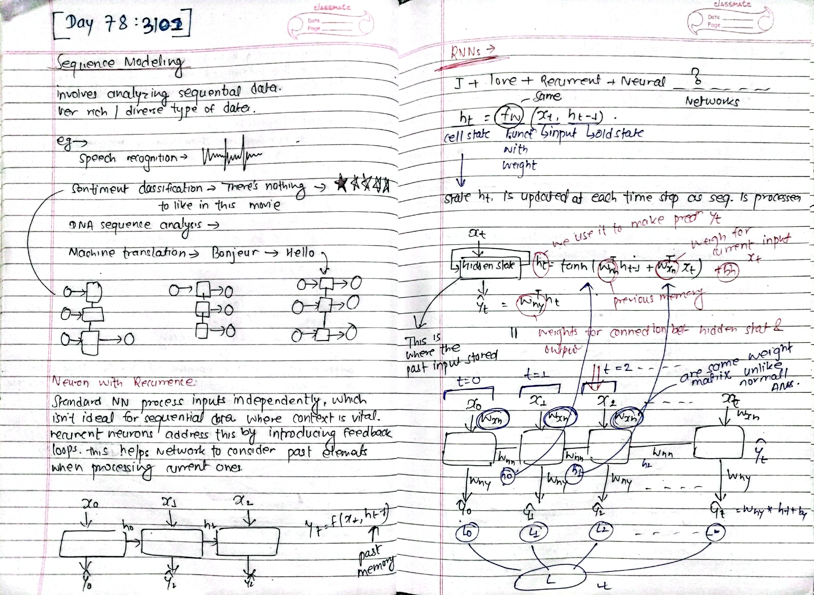
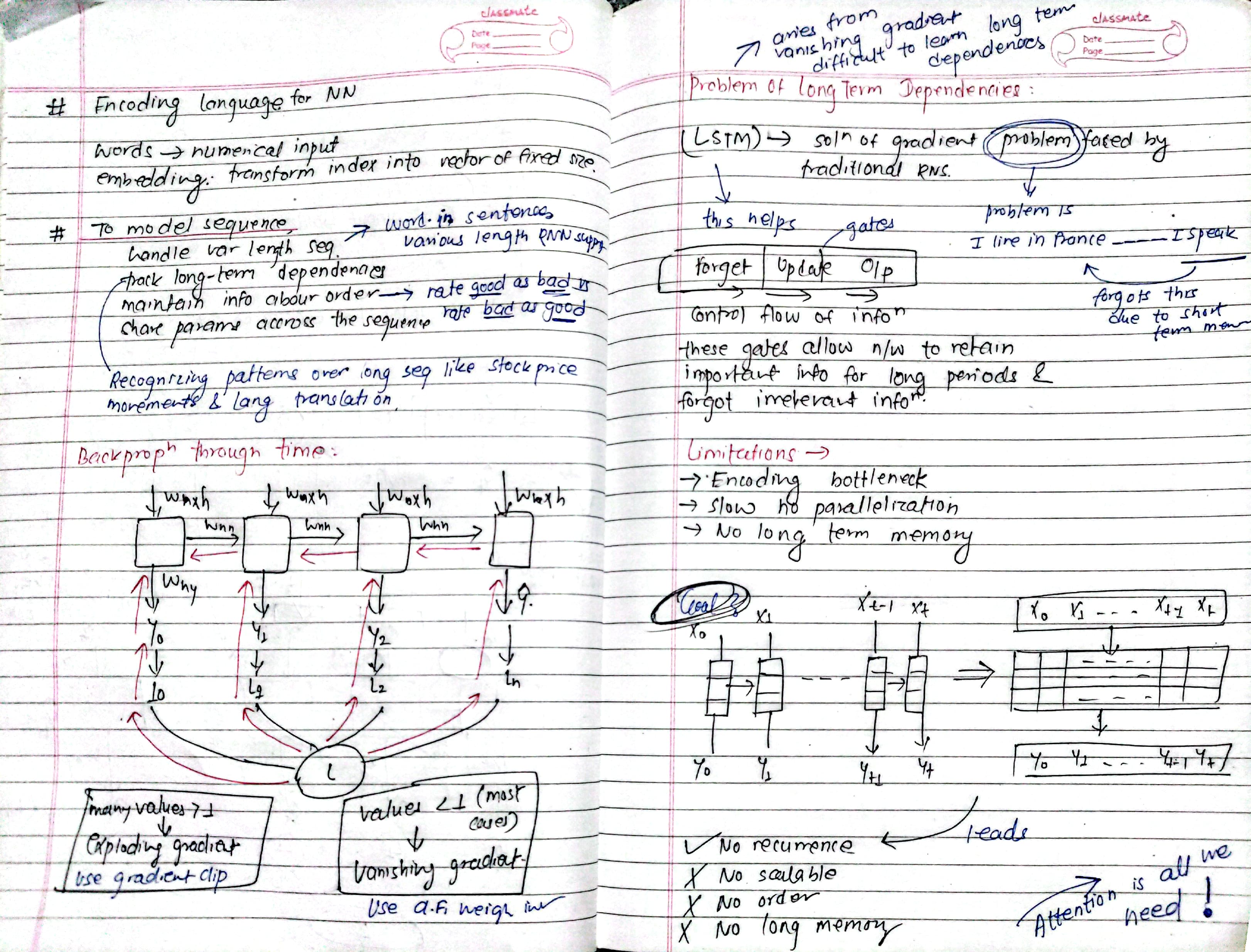
Implementation Preview
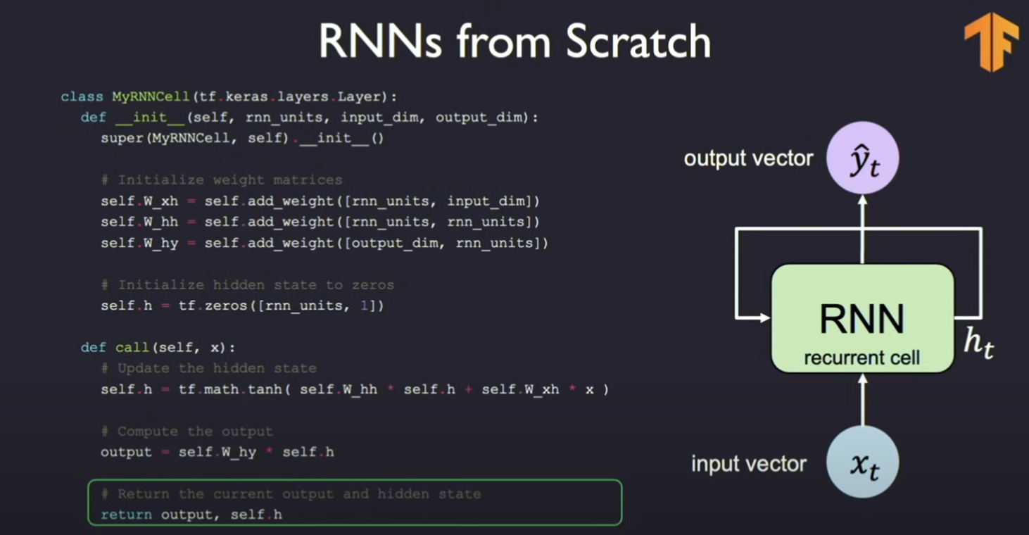
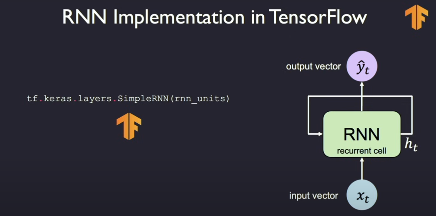
Day 79: Transformers , Attention - Just Overview
Transformers replace RNNs by using self-attention, enabling parallel processing and handling long-range dependencies efficiently. Introduced in "Attention Is All You Need" (2017), they power models like BERT and GPT.
Self-attention computes Query (Q), Key (K), and Value (V) matrices to determine word relationships. Multi-head attention allows the model to capture different contextual meanings.
The transformer consists of encoder-decoder blocks with self-attention, feed-forward layers, and normalization. Encoders learn representations, while decoders generate sequences.
Transformers are used in chatbots, translation, search engines, and AI coding assistants. Key models include BERT (bi-directional understanding), GPT (text generation), and T5 (text-to-text tasks).
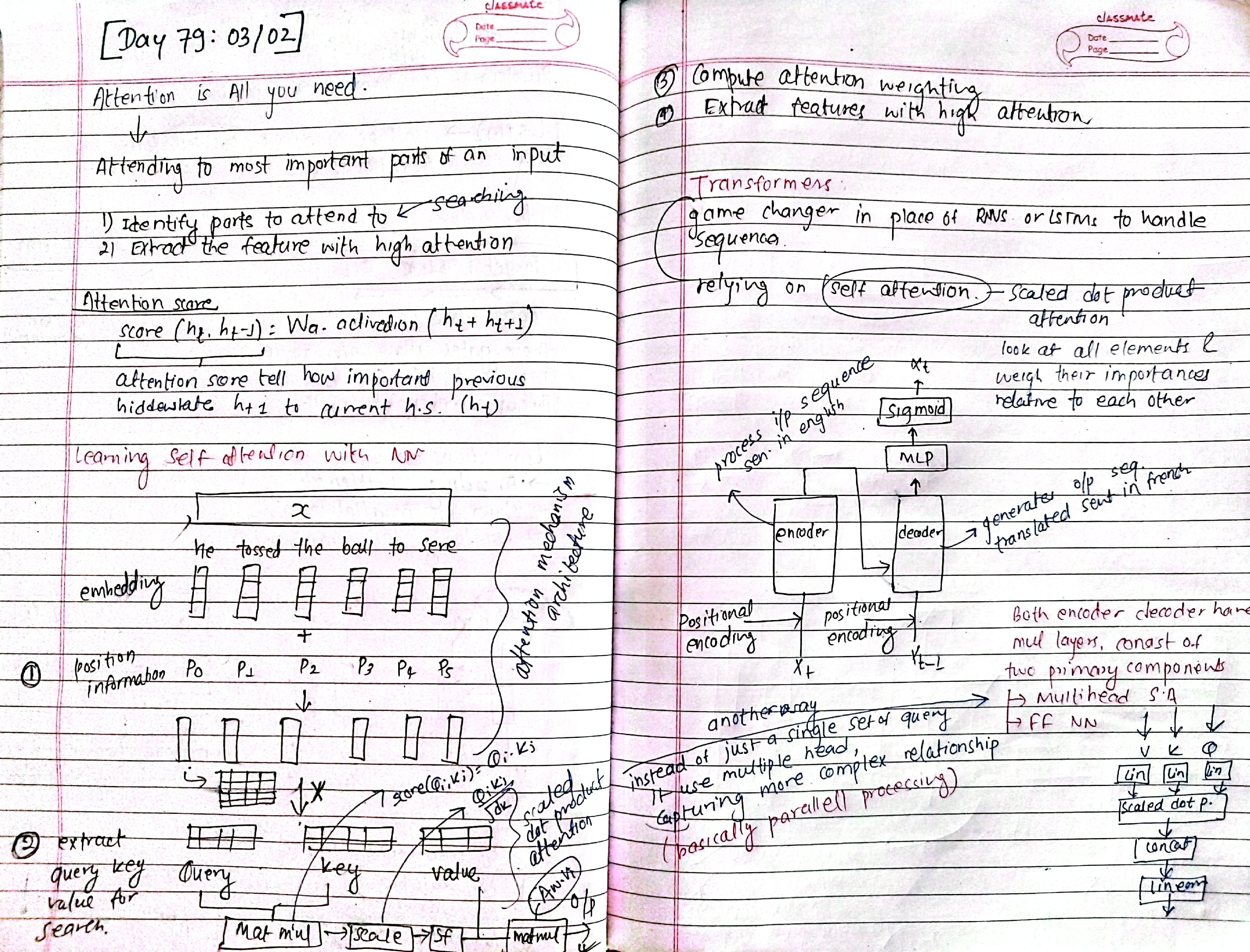
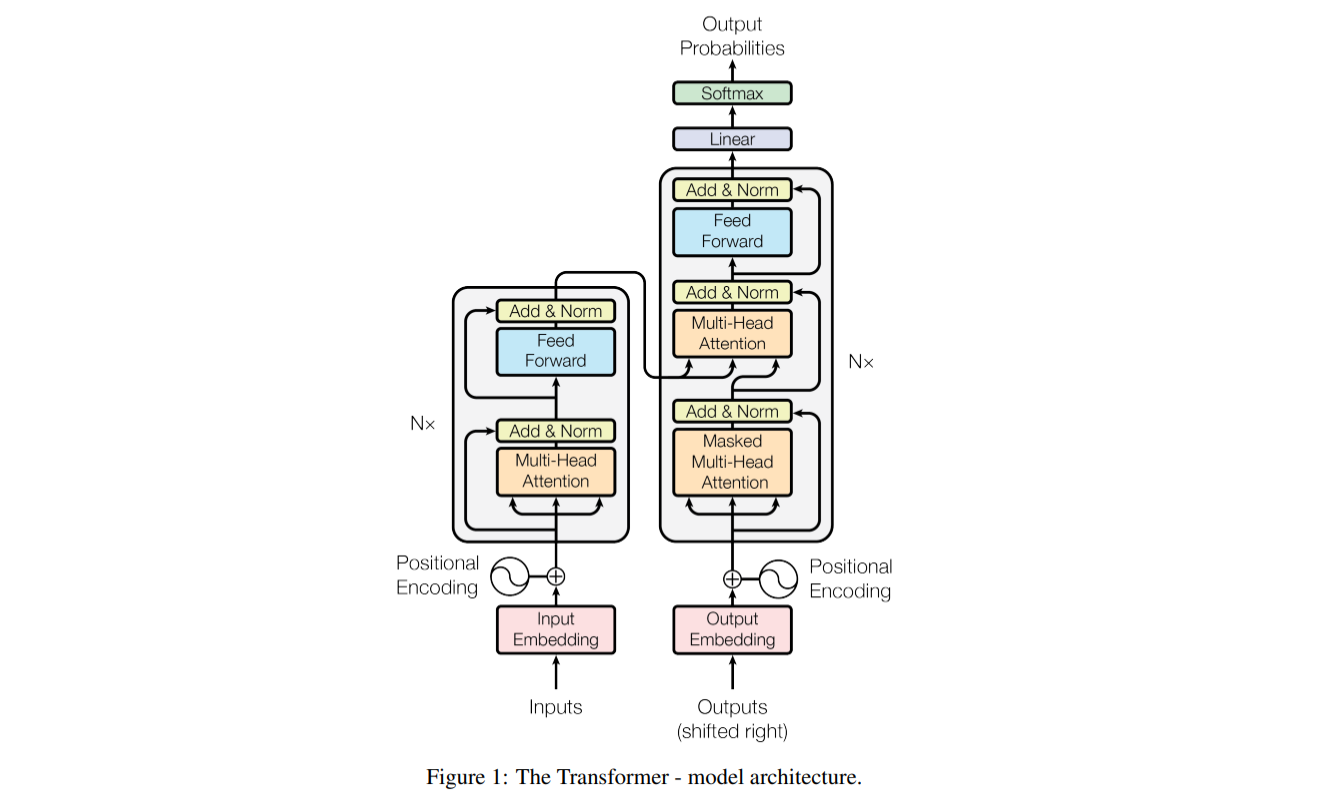
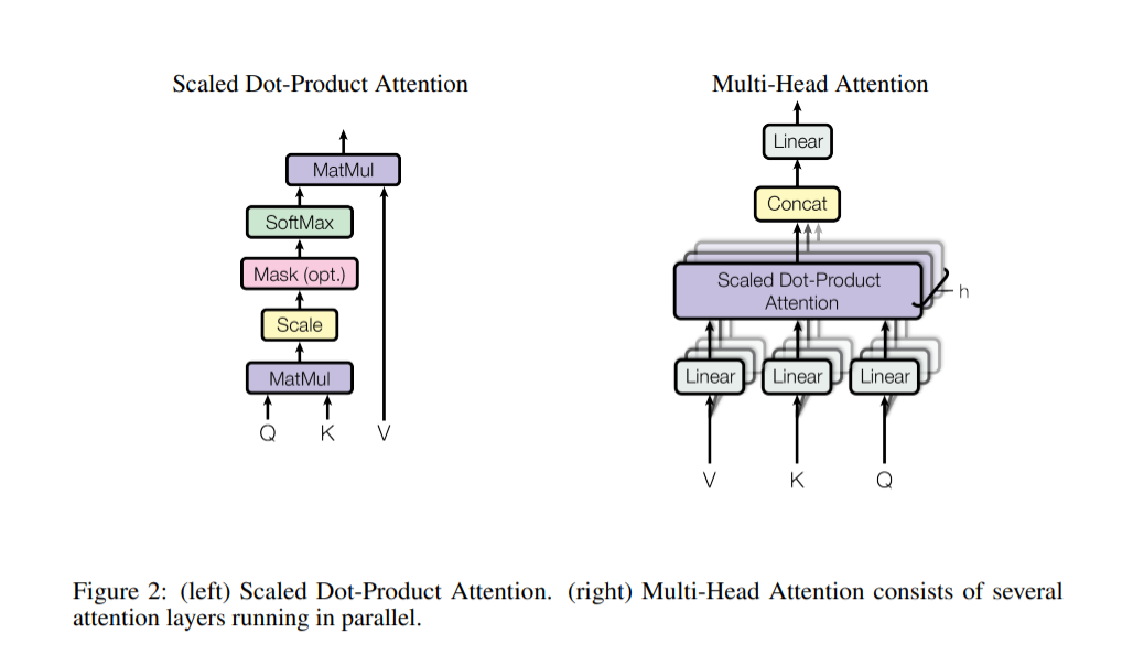
Day 80: CNNs - Just Overview Part 1
- Computer vision enables machines to interpret visual data.
- Used in self-driving cars, medical imaging, surveillance, AR.
What Computers "See"
- Images are matrices of pixel values (grayscale: single matrix, RGB: 3 matrices).
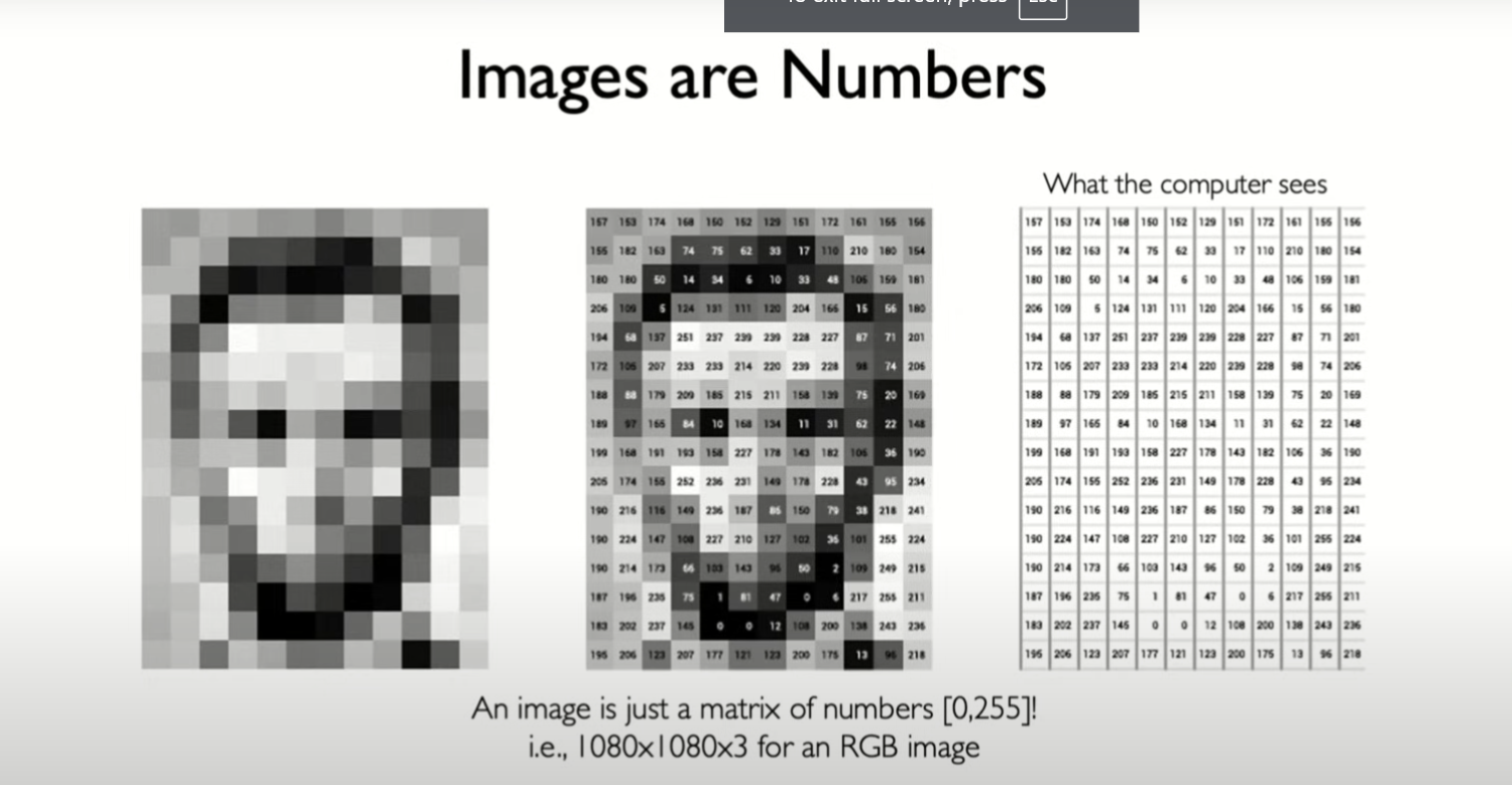
Feature Extraction & Convolution
- CNNs learn features like edges, textures, and shapes automatically.
- Convolution: uses filters (kernels) to extract patterns from images.
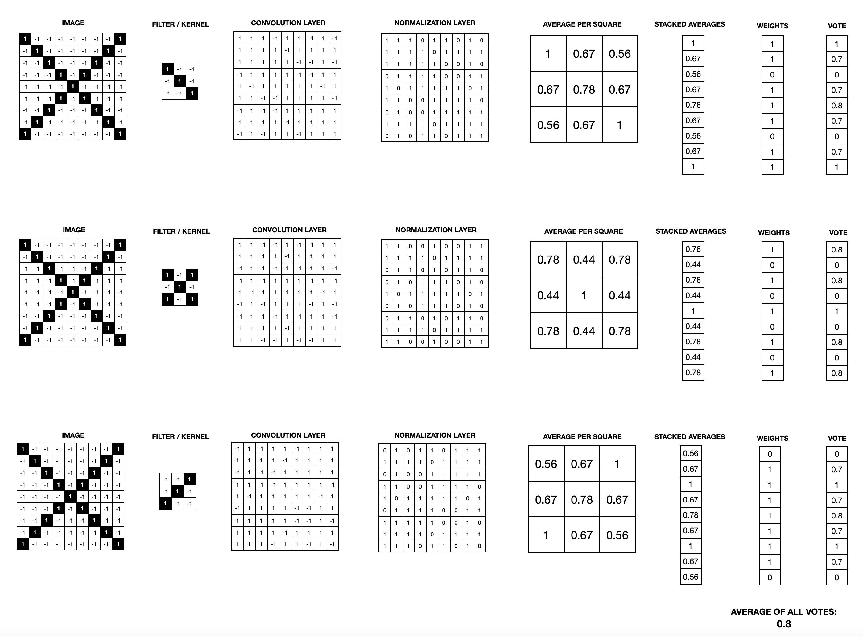
- Example Kernel (Edge Detection - traditional filter):
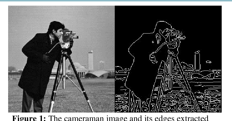
CNN Architecture
- Convolution Layers: detect patterns.
- ReLU Activation: makes model non-linear.
- Pooling Layers: reduce size, keep key features.
- Fully Connected Layers: classify objects.
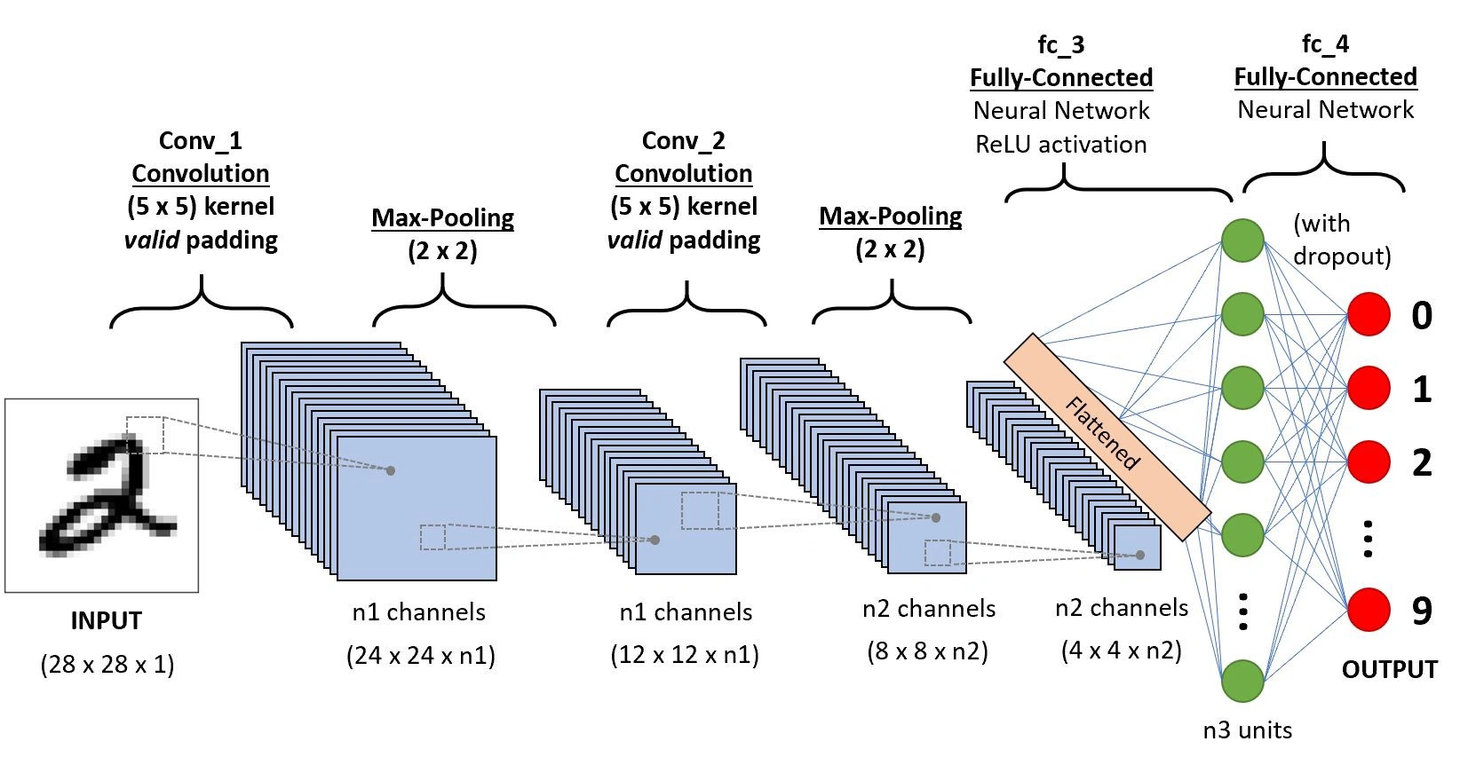
Object Detection
use yolo when speed matters more than precision (e.g., real-time apps).
use rcnn when accuracy is critical and speed isn’t a constraint.
use faster rcnn for a balance between accuracy and speed.
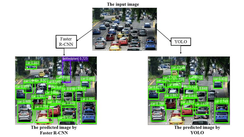
Self-Driving Cars
- CNNs help detect lanes, pedestrians, and traffic signs.
- End-to-end models predict steering angles using video input.

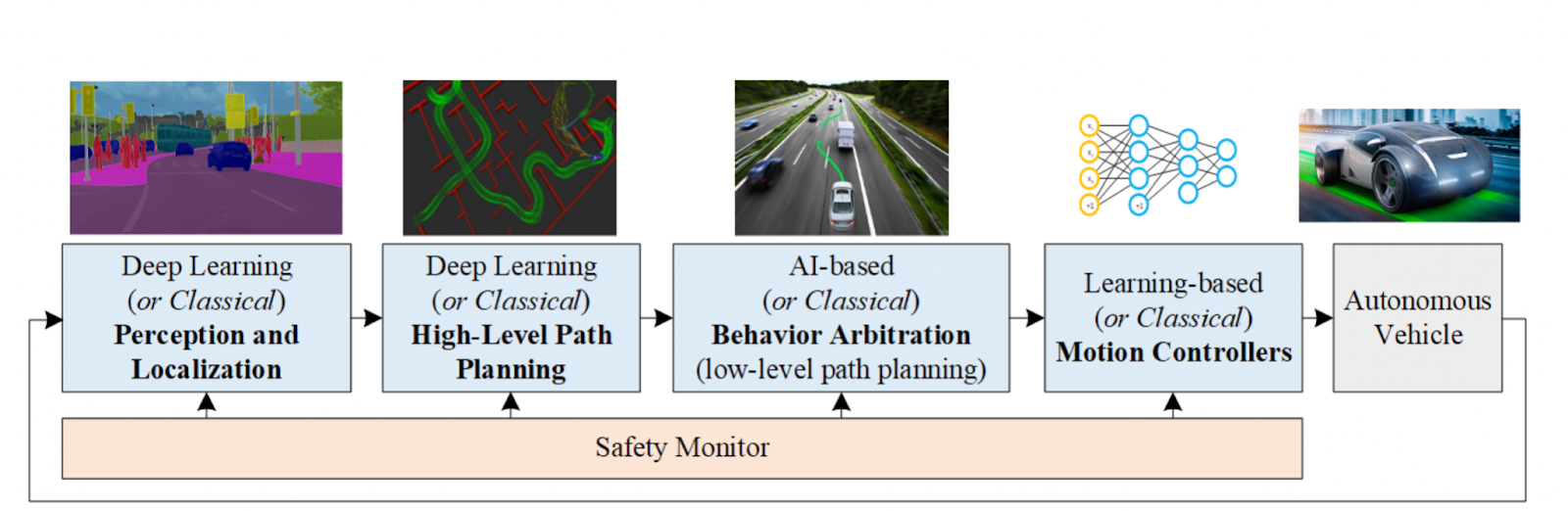
Day 81: CNNs - Just Overview Part 2
yesterday, i watched a video on cnn. the goal was just to explore it for a day, but i feel like this is an interesting topic. so today, i want to learn more—like, in-depth—about the feature extraction part, which i find the most interesting aspect of cnn.
i learned to use relu and understood convolution layers and how they work yesterday. but today, i learned about pooling and how it reduces the size. i also explored the classification process in more depth.
notes:
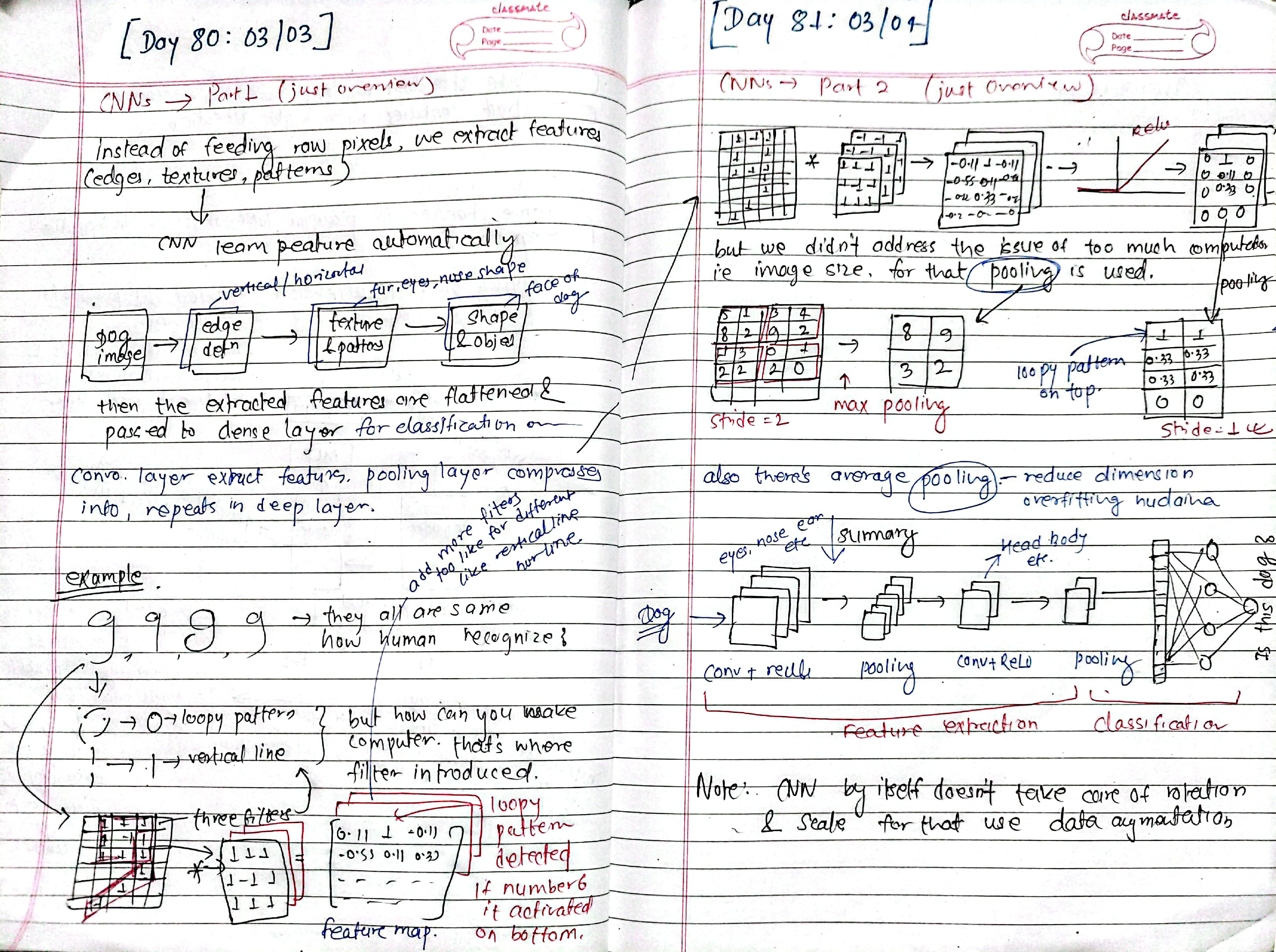 note: cnn by itself doesn't handle rotation and scaling well. for that, use data augmentation.
Day 82: Deep Generative modeling - Just overview
Watched this single video : https://www.youtube.com/watch?v=Dmm4UG-6jxA&t=3242s
today’s deep dive into generative models gave me a solid grasp of how ai can not only recognize patterns but also create new data from scratch. these models are the backbone of modern generative ai, and understanding them is key to keeping up with the field.
Generative models: what they do
- they don’t just classify or analyze data; they generate entirely new data that resembles what they learned from.
- examples include autoencoders, variational autoencoders (VAEs), GANs, and diffusion models—each with its own strengths.
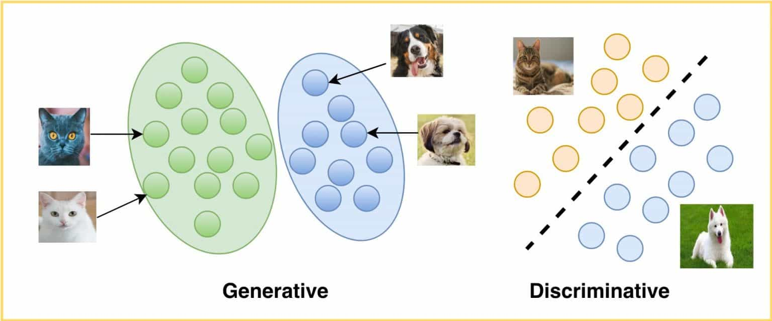
Latent variable models: finding the hidden structure
- autoencoders learn to compress data into lower-dimensional representations and then reconstruct it.
- vaes take this further by adding randomness, making them better at generating diverse outputs instead of just memorizing patterns.
- plato’s cave analogy clicked here—observed data is like shadows on a wall, while latent variables represent the actual objects casting those shadows.
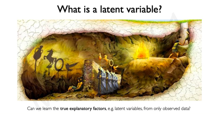
Generative adversarial networks (GANs): competition makes better results
- a generator creates fake data, while a discriminator tries to catch the fakes.
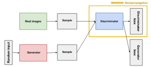
- through constant feedback, both improve, leading to highly realistic outputs.
- training is tricky—imbalanced learning can cause mode collapse, where the generator keeps making similar outputs instead of diverse ones.
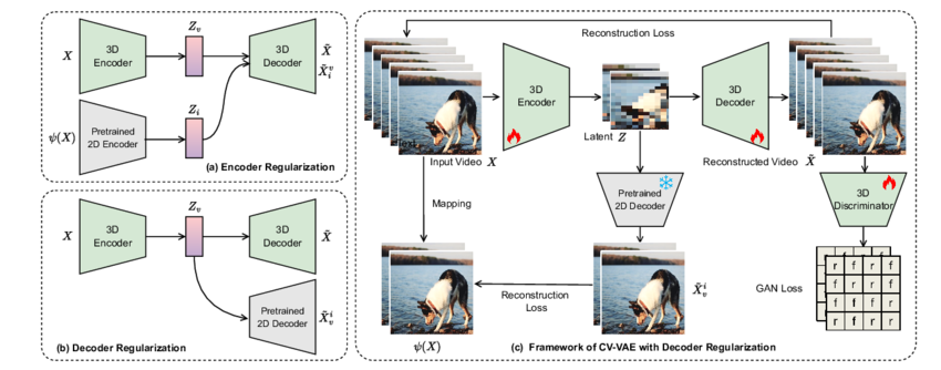
Regularization & structure in vaes
- forcing the latent space into a structured distribution (often gaussian) helps ensure smoothness and continuity, making vaes more useful for controlled generation.
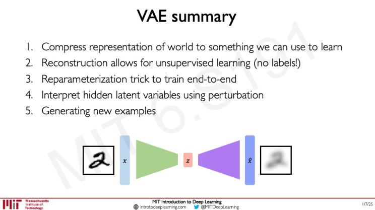
Applications beyond images
- these models aren't just for ai art—they power speech synthesis, text generation, and even domain adaptation (like CycleGAN for translating images without paired data).
Diffusion models: a new generative powerhouse
- instead of generating images all at once (like GANs), diffusion models gradually refine noise into meaningful images.
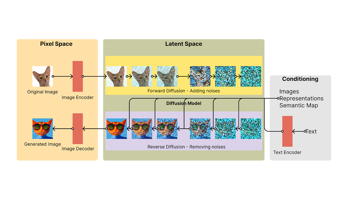
- they’re more stable and produce higher-quality results, making them the future of generative ai.
Day 83: Reinforcement Learning - Just Overview
with the help of this video: https://www.youtube.com/watch?v=8JVRbHAVCws&t=3242s
-
explored key concepts of reinforcement learning (RL), including Q-learning and policy learning algorithms.
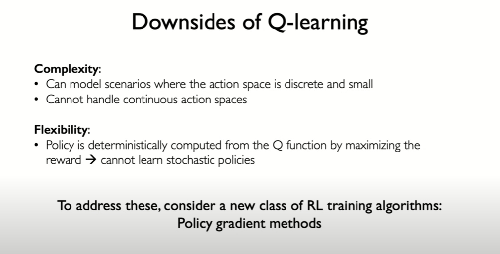
-
dived into Deep Q Networks (DQN) and their role in handling complex environments, like Atari games.
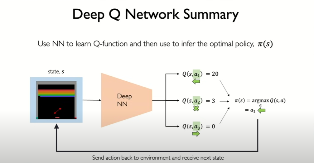
-
understood the difference between discrete and continuous actions and how they impact RL models.
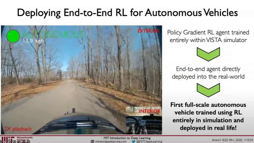
-
learned about real-world applications of RL, from robotics to game AI, and cutting-edge technologies like AlphaGo and MuZero.
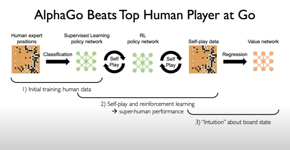
-
explored training techniques like policy gradients and how they improve decision-making in RL agents.
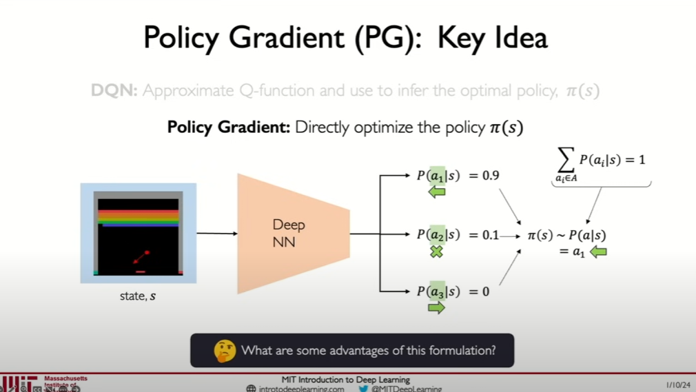
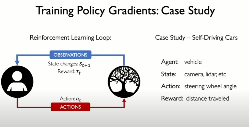
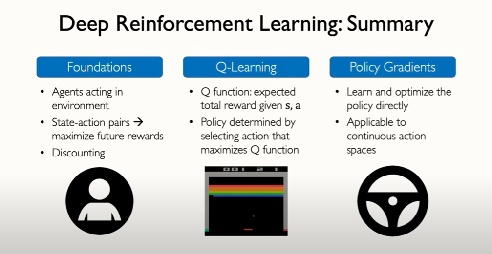
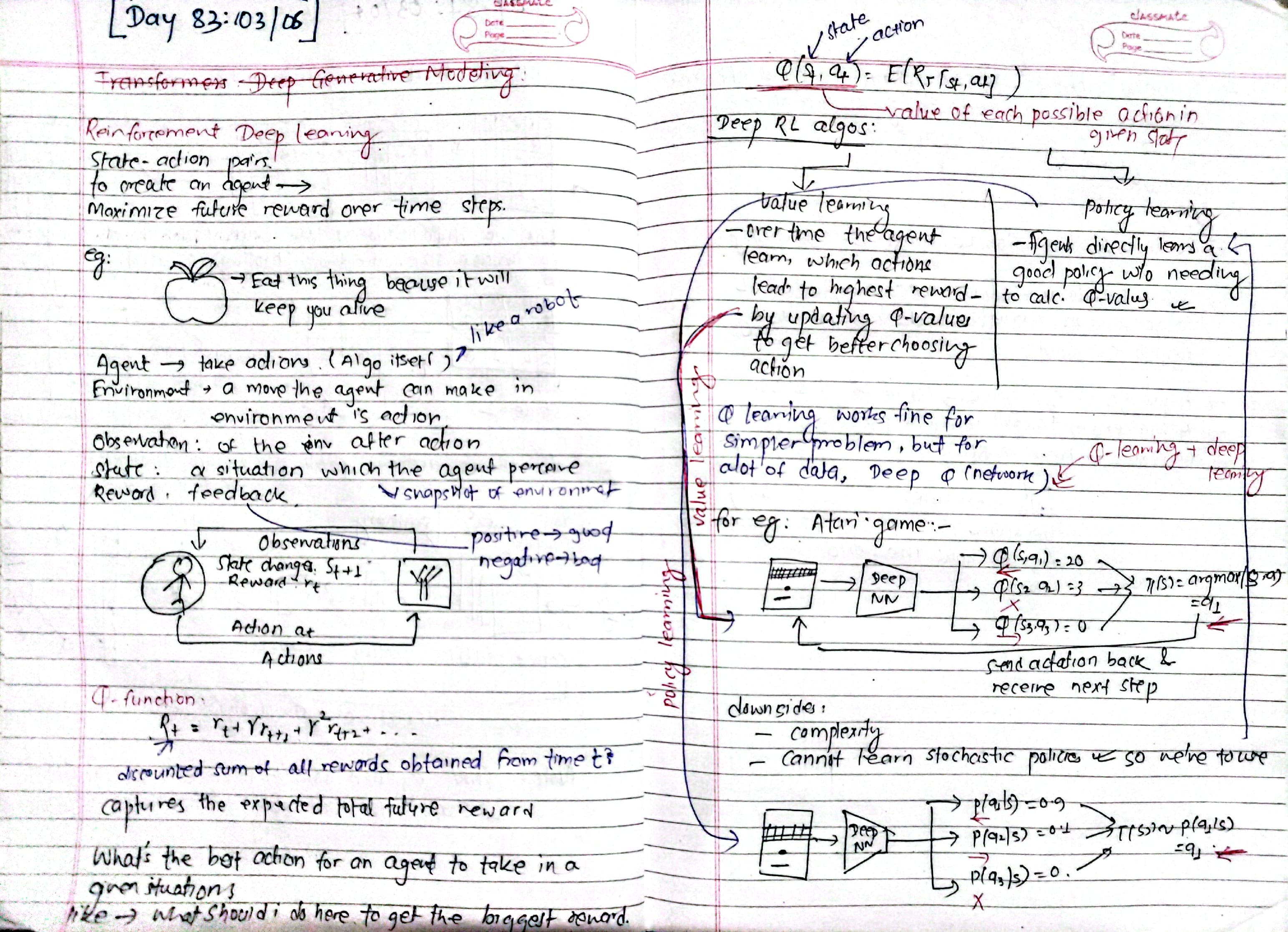
Day 84: Deep learning: challenges & new frontiers - Just Overvview
Video Link: https://www.youtube.com/watch?v=N1fbskTpwZ0&t=3021s
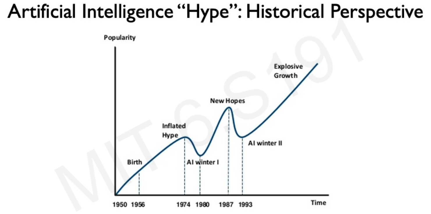
- neural network failure modes – ai can fail unpredictably, often overconfident in wrong answers.
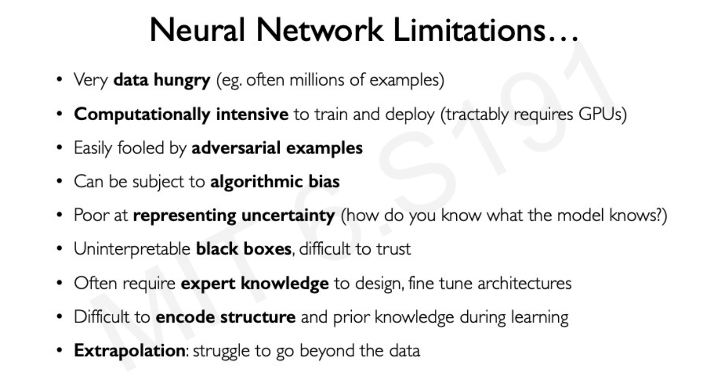
- uncertainty in deep learning – models lack awareness of their own mistakes, leading to unreliable predictions.
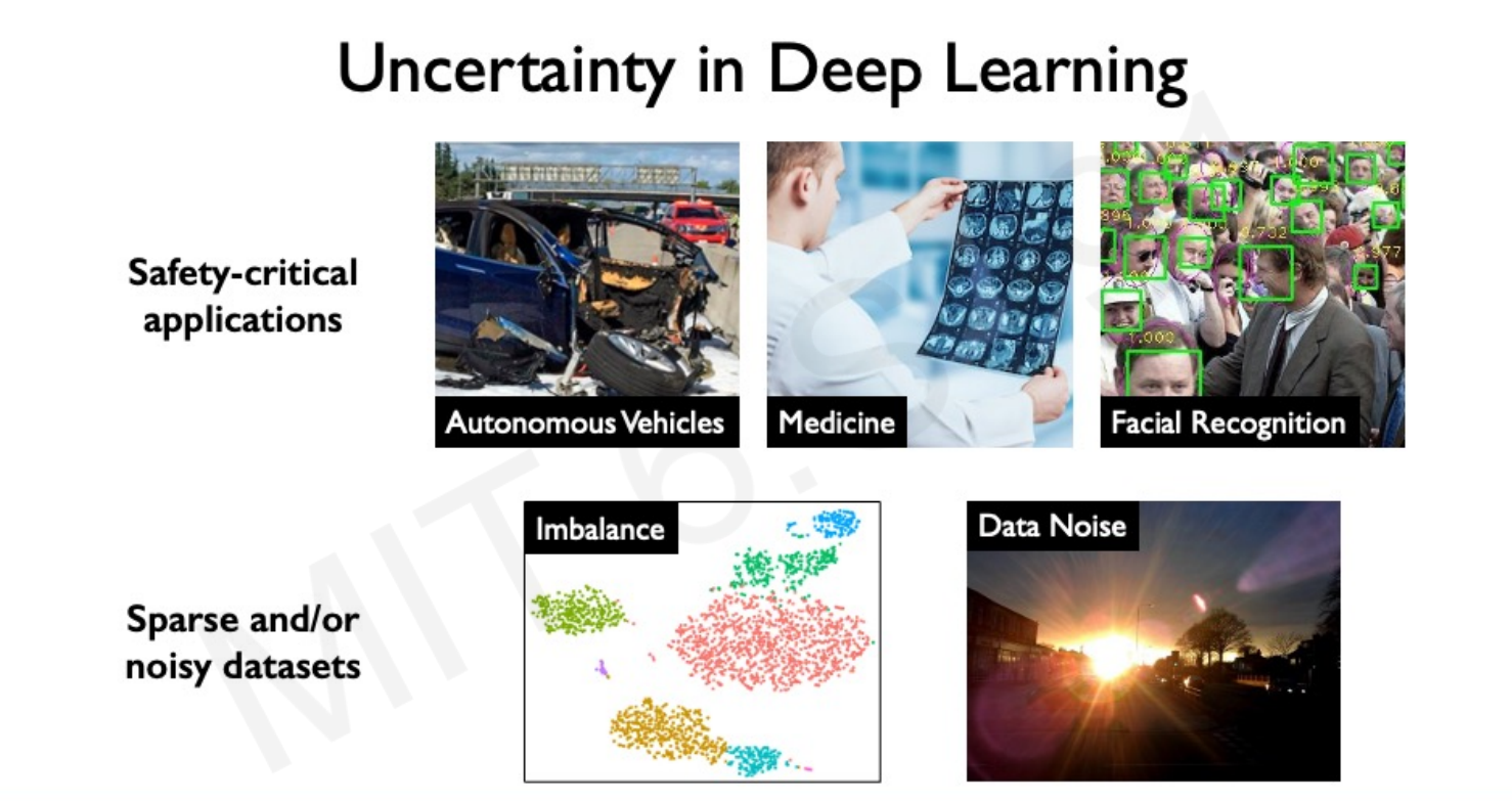
- adversarial attacks – tiny changes in input can trick ai into making completely wrong decisions.
- algorithmic bias – ai inherits and amplifies biases from training data, leading to unfair outcomes.
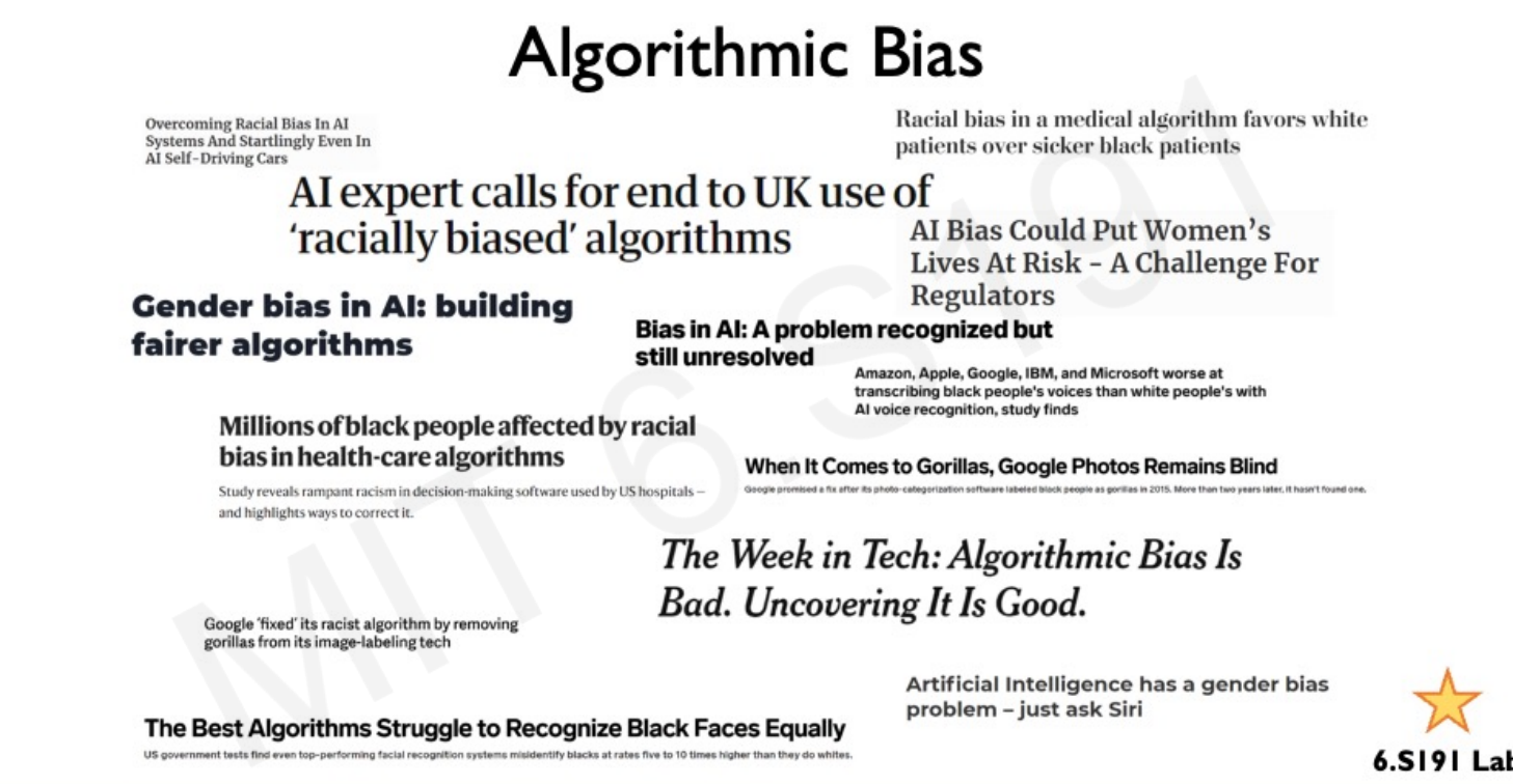
generative ai & diffusion models
- the landscape – diffusion models are replacing GANs in high-quality image generation.
- diffusion process – gradually add noise to data and train a model to reverse it.
- noising & denoising – AI learns to reconstruct images by stepwise noise removal.
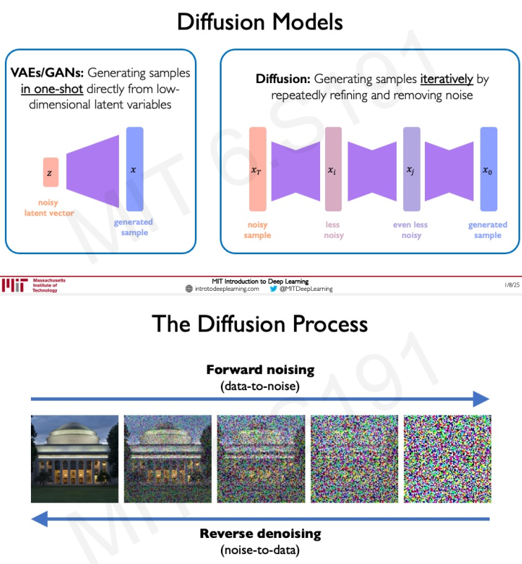
- text to image, beyond images – models like DALL·E generate images, but AI is expanding into text, music, and 3D.
large language models (LLMs)
- using llms to generate text – models predict words to generate human-like text.
- limitations – hallucinations, bias, and lack of real understanding.
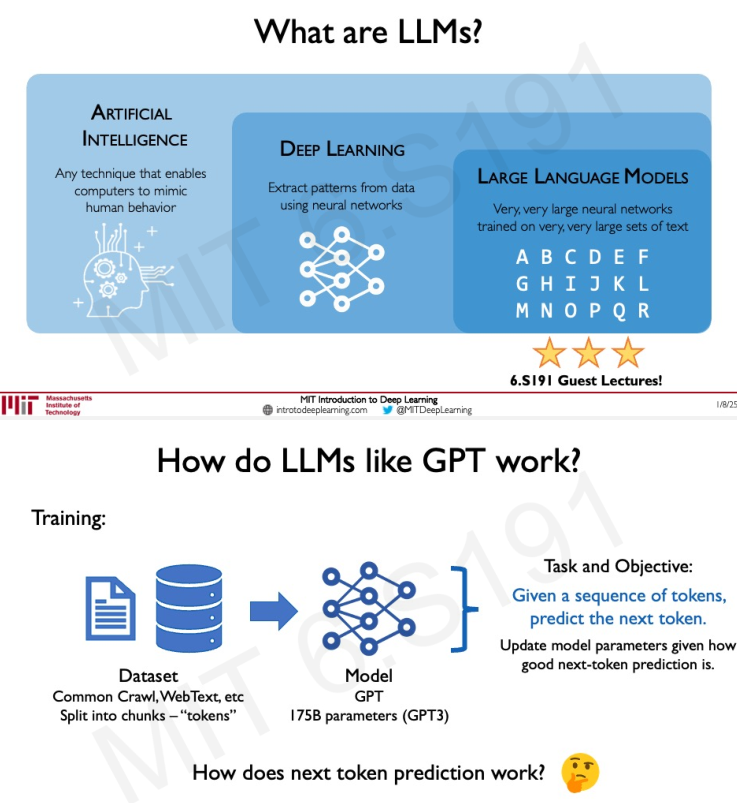
- more parameters = better performance, but higher computational cost.
- how they work – transformers + attention mechanism process and generate context-aware text
Day 85: Early Stopping, Normalizing Inputs, Dropout
These are the techniques i will cover in upcoming days:
-
Vanishing Gradients
- Activation Functions
- Weight Initialization
-
Overfitting
- Reduce Complexity/Increase Data
- Dropout Layers
- Regularization (L1 & L2)
- Early Stopping
-
Normalization
- Normalizing inputs
- Batch Normalization
- Normalizing Activations
-
Gradient Checking and Clipping
-
Optimizers
- Momentum
- Adagrad
- RMSprop
-
Learning rate scheduling
-
Hyperparameter Tuning
- No. of hidden layers
- Nodes/layer
- Batch size
Today, I explored Early Stopping, Normalizing Inputs, and Dropout techniques for improving neural network performance.
- Early Stopping: Prevents overfitting by halting training when validation performance drops.
- Normalizing Inputs: Scales features to a consistent range, aiding in faster and more stable learning.
- Dropout: Reduces overfitting by randomly deactivating neurons during training, forcing the model to generalize better.
Notebook: Dropout on Regression
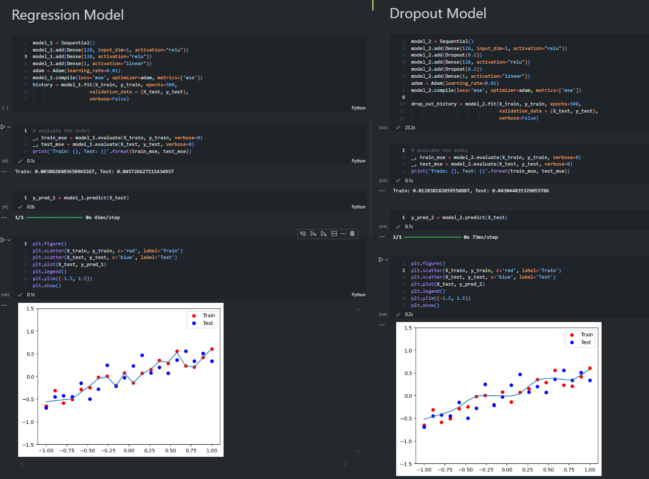 Notebook: Dropout on Classification
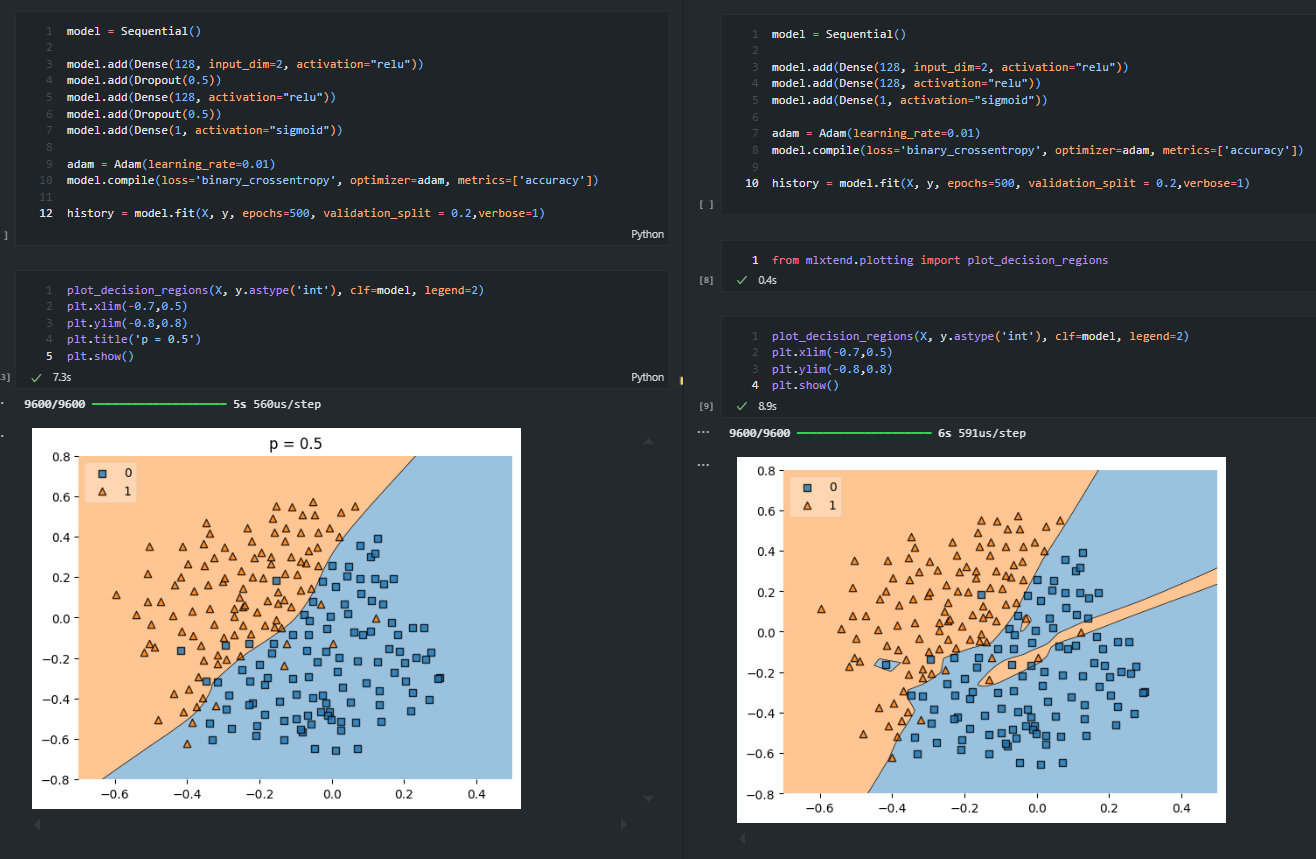
Day 86: Regularization, Quantization
L1 and L2 regularization are typically used for smaller networks. For larger networks, it is better to use neural network-specific regularization which is dropout regularization.
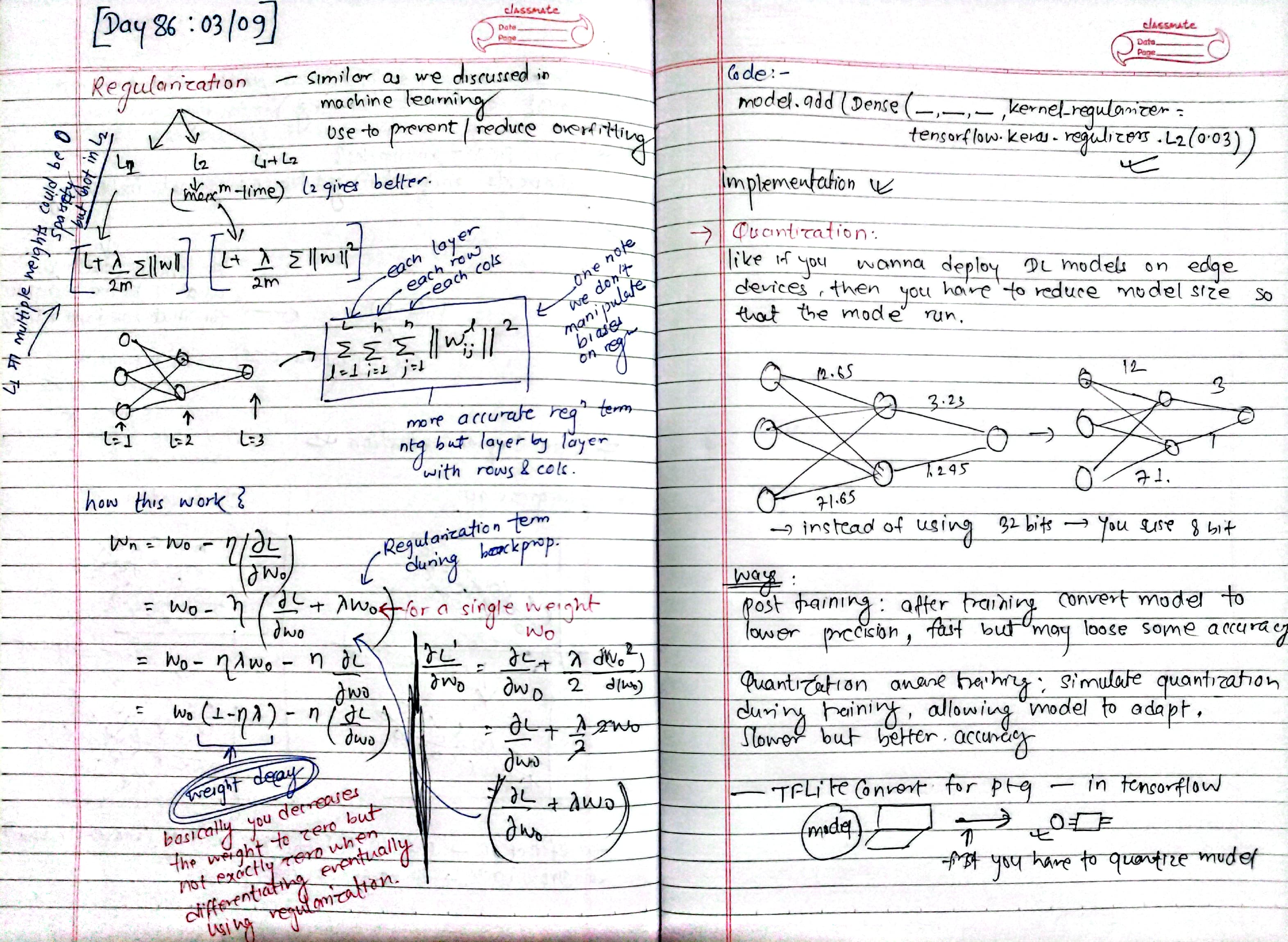
An evaluation procedure must be used when using a regularizer to monitor that regularization process. For this, we can plot model performance against the number of epochs during the training process.
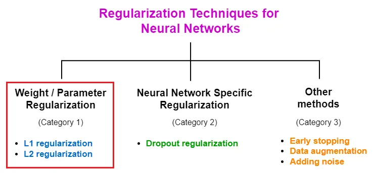
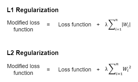
Notebook: without Regularization vs Applying Regularization
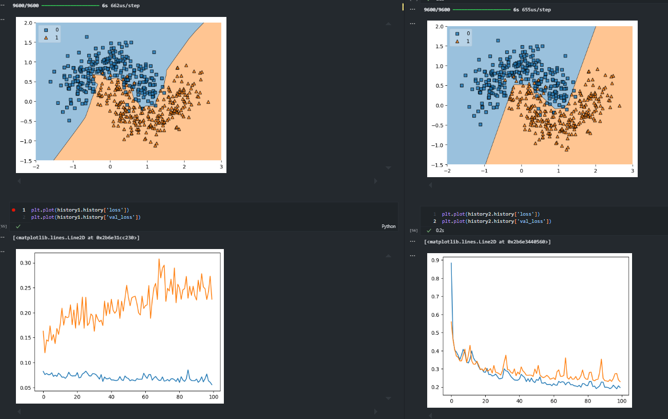
Quantization:
quantization in deep learning reduces the precision of numbers in a model to save memory and speed up processing. it can be done in two ways: post-training quantization (ptq), which converts the model to lower precision after training for faster performance but may lose some accuracy, and quantization-aware training (qat), where quantization is simulated during training, resulting in better accuracy but requiring more time. frameworks like TensorFlow provide tools for both methods to help deploy lighter and faster models.
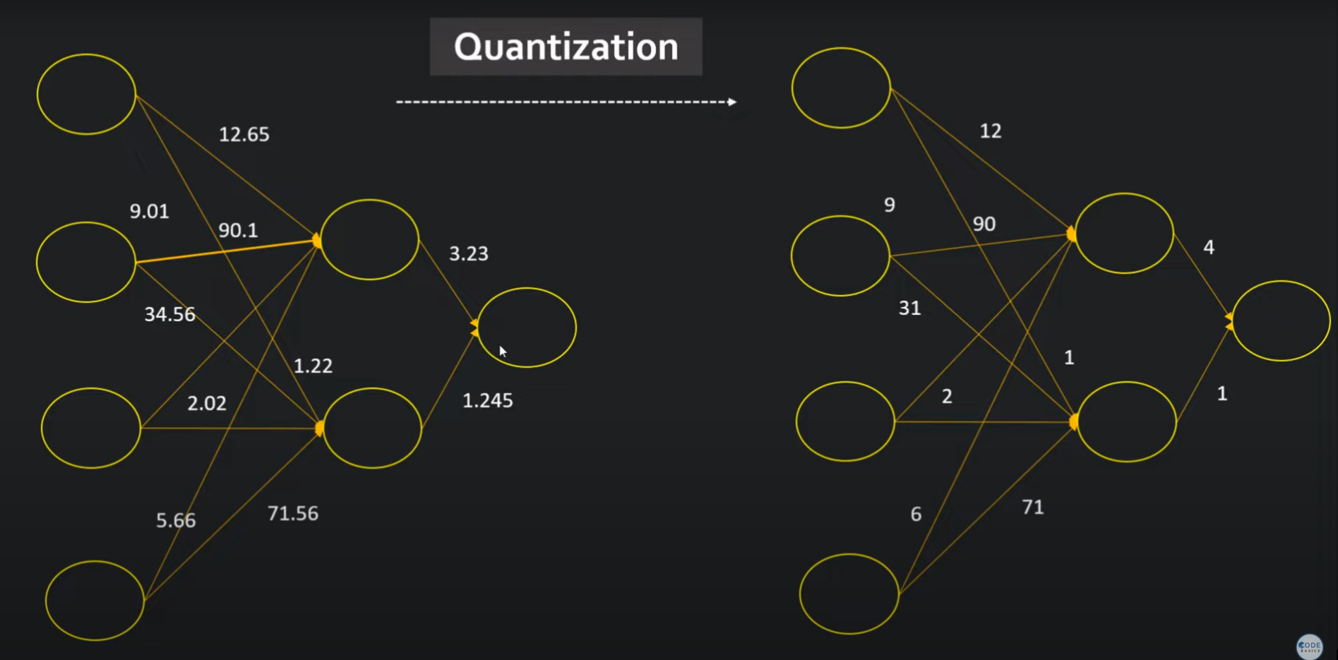
Day 87 - Activation Functions - Revisited
why needed? introduce non-linearity to capture complex patterns.
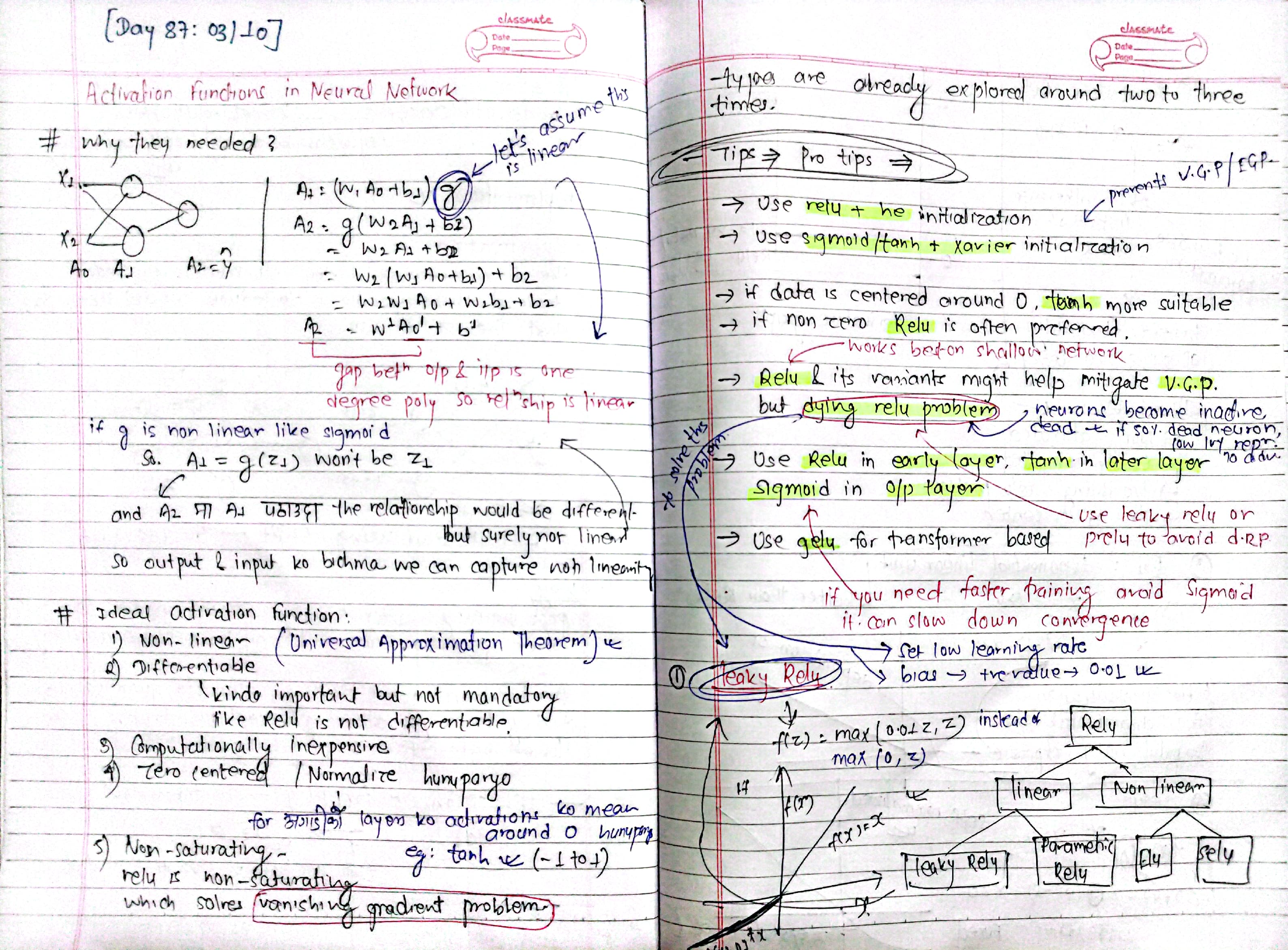
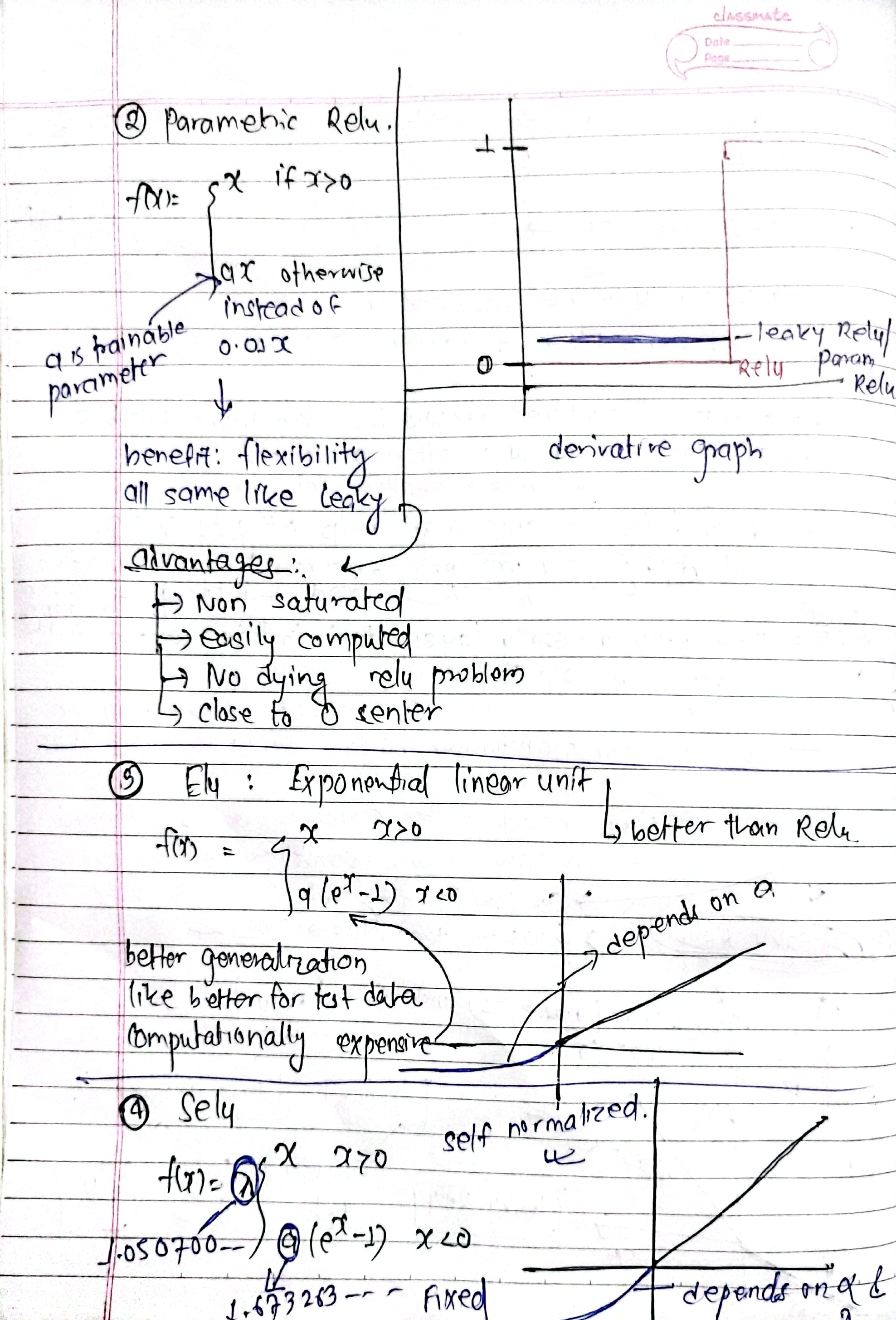 ideal properties: non-linear, differentiable, computationally inexpensive, zero-centered, non-saturating.
- use relu + he init, sigmoid/tanh + xavier init.
- relu in early layers, tanh or sigmoid in later/output layers.
- prefer gelu for transformers.
- avoid dying relu with leaky relu or prelu.
relu: fast, simple but can die.
leaky relu: small slope for negatives, avoids dead neurons.
prelu: learnable slope, more flexible.
elu: better generalization, but expensive.
selu: self-normalizing, good for deep nets.
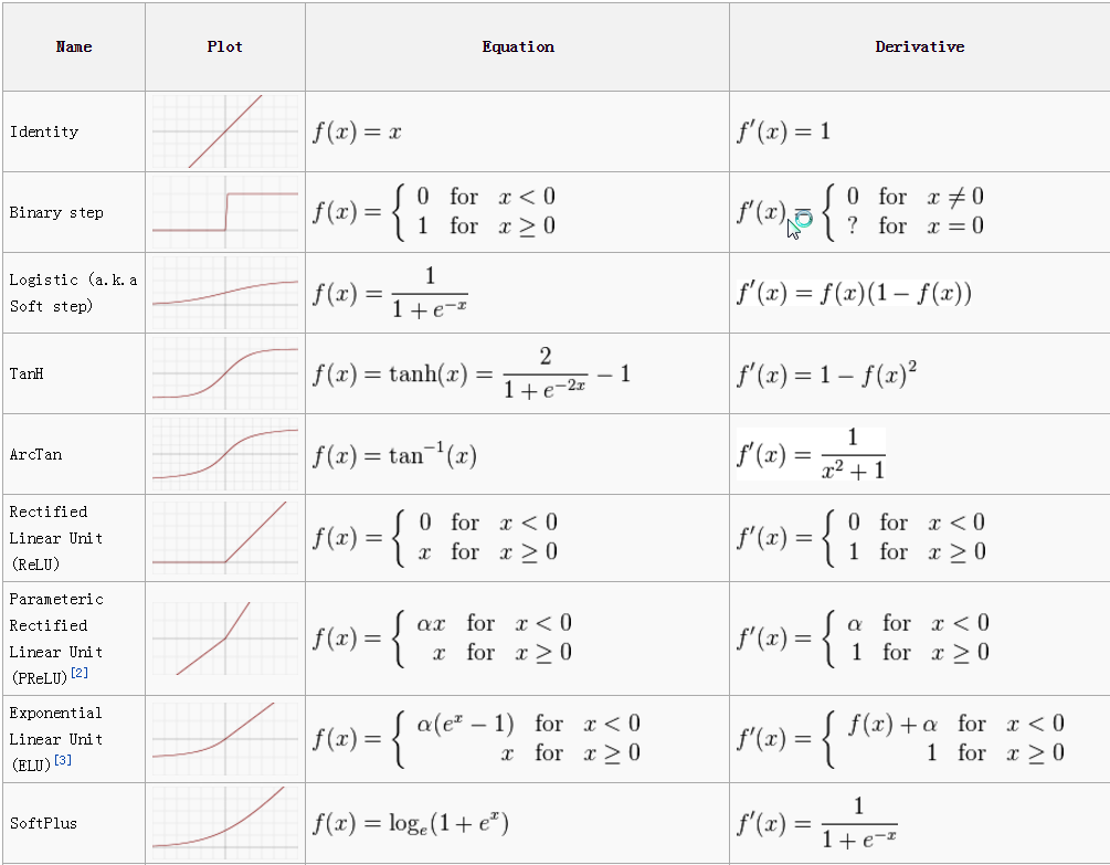
Day 88: Weight Initialization
Zero Init: All weights as zero → no learning (same gradients).
weights = np.zeros((input_size, output_size))
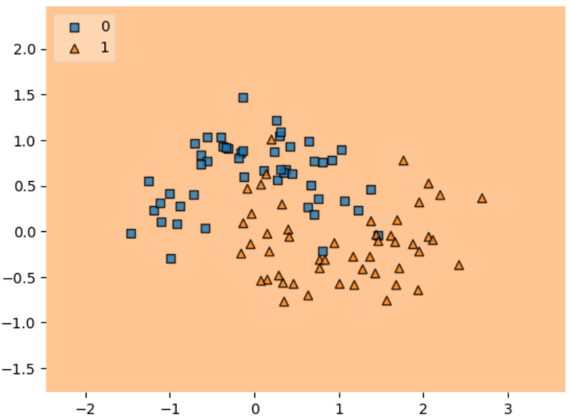
One Init: All weights as one → same issue, no symmetry breaking.
weights = np.ones((input_size, output_size))
✅ Random Init: Small random values.
weights = np.random.randn(input_size, output_size) * 0.01
✅ Xavier Init (for tanh/sigmoid):
weights = np.random.randn(input_size, output_size) * np.sqrt(1 / input_size)
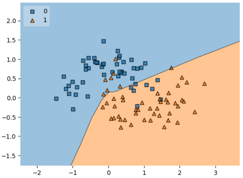
✅ He Init (for ReLU):
weights = np.random.randn(input_size, output_size) * np.sqrt(2 / input_si
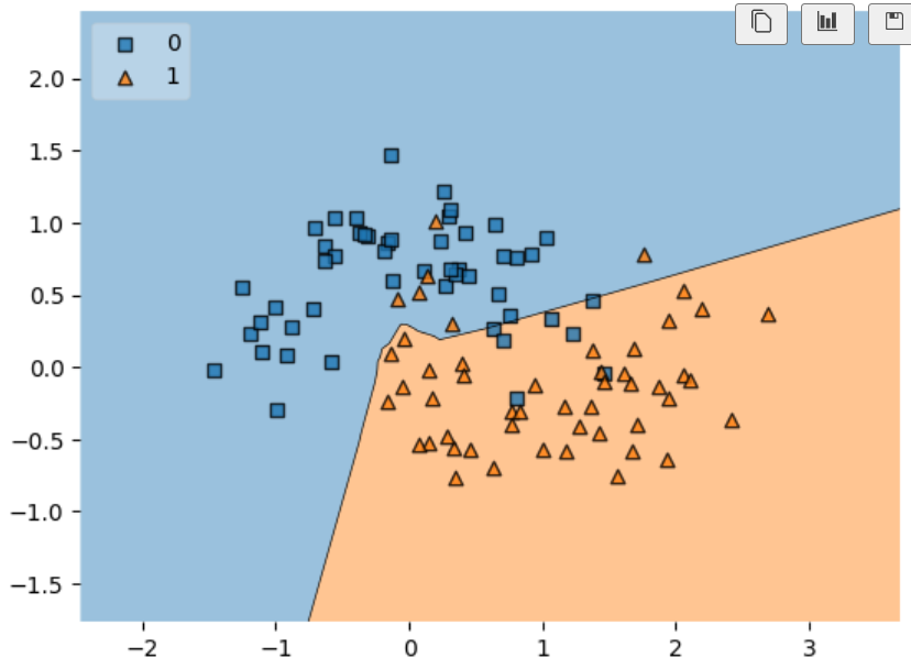
Notebook: Weight Initialization
Notebook: Xavier and He initialization
Notes:
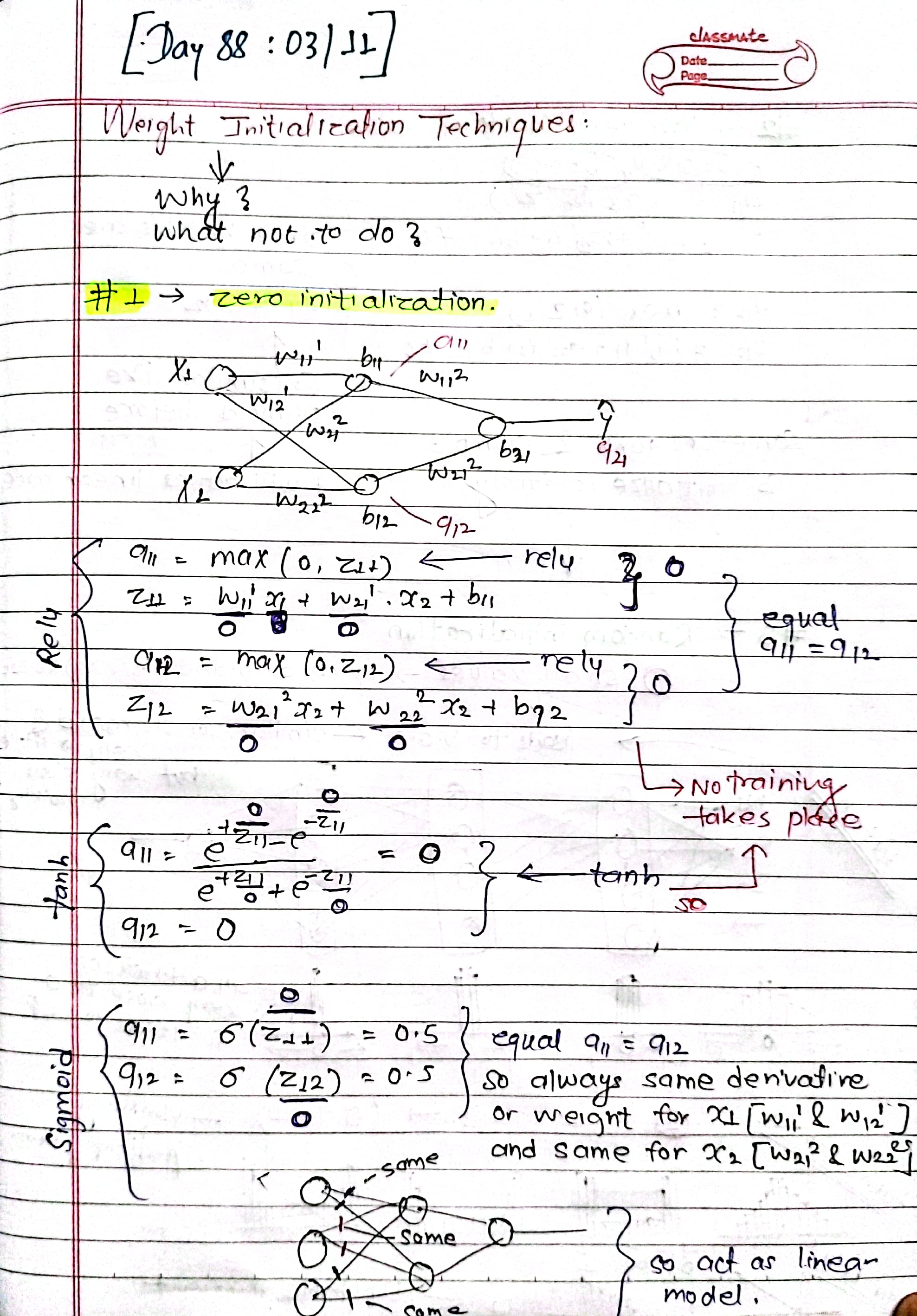
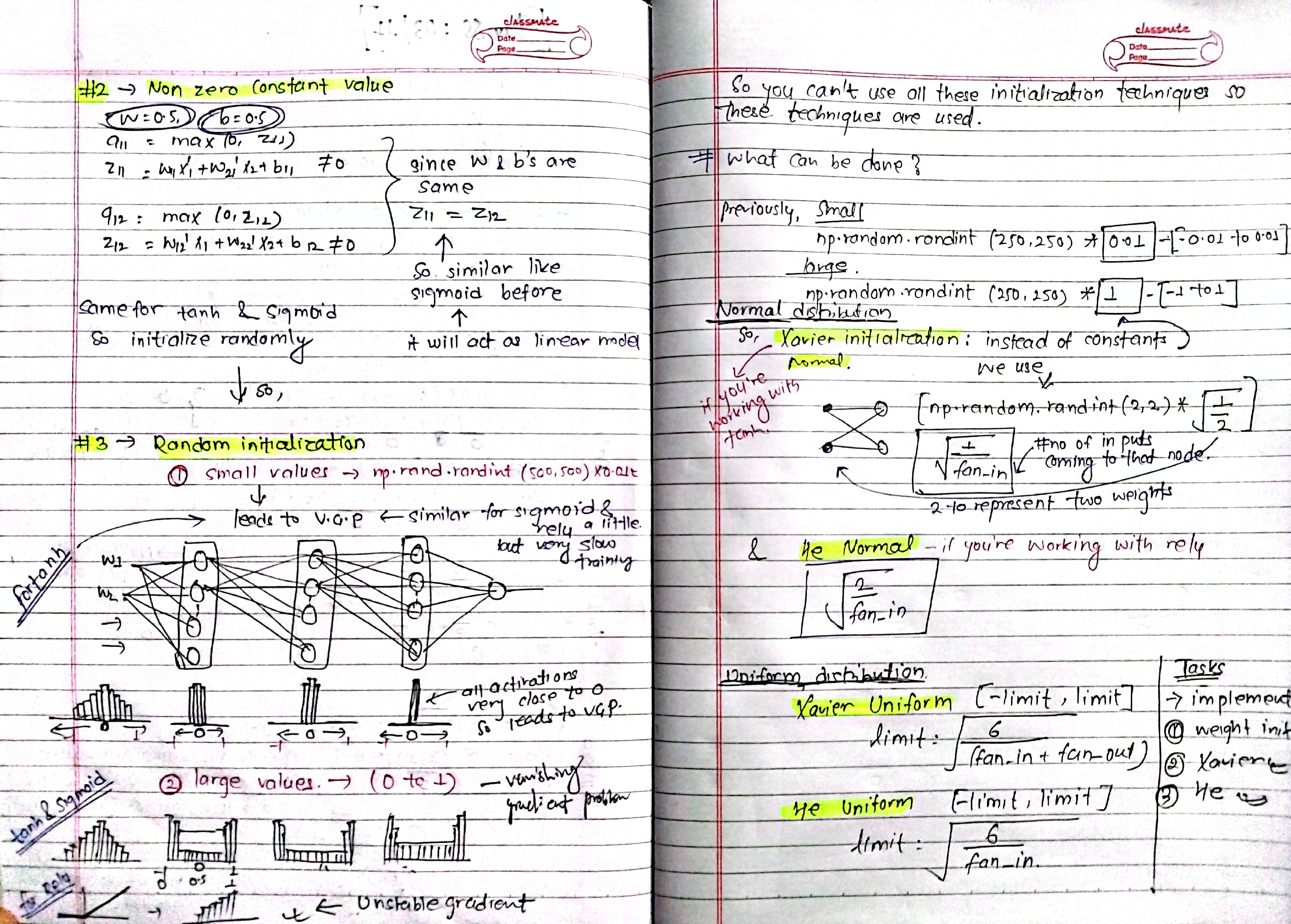
Day 89: Deeep Learning Optimizers
- Gradient Descent: Fundamental optimizer that updates weights by moving in the opposite direction of the gradient of the loss function w.r.t. the weights. It's basic but effective for many problems.
from tensorflow.keras.optimizers import SGD
optimizer = SGD(learning_rate=0.01)
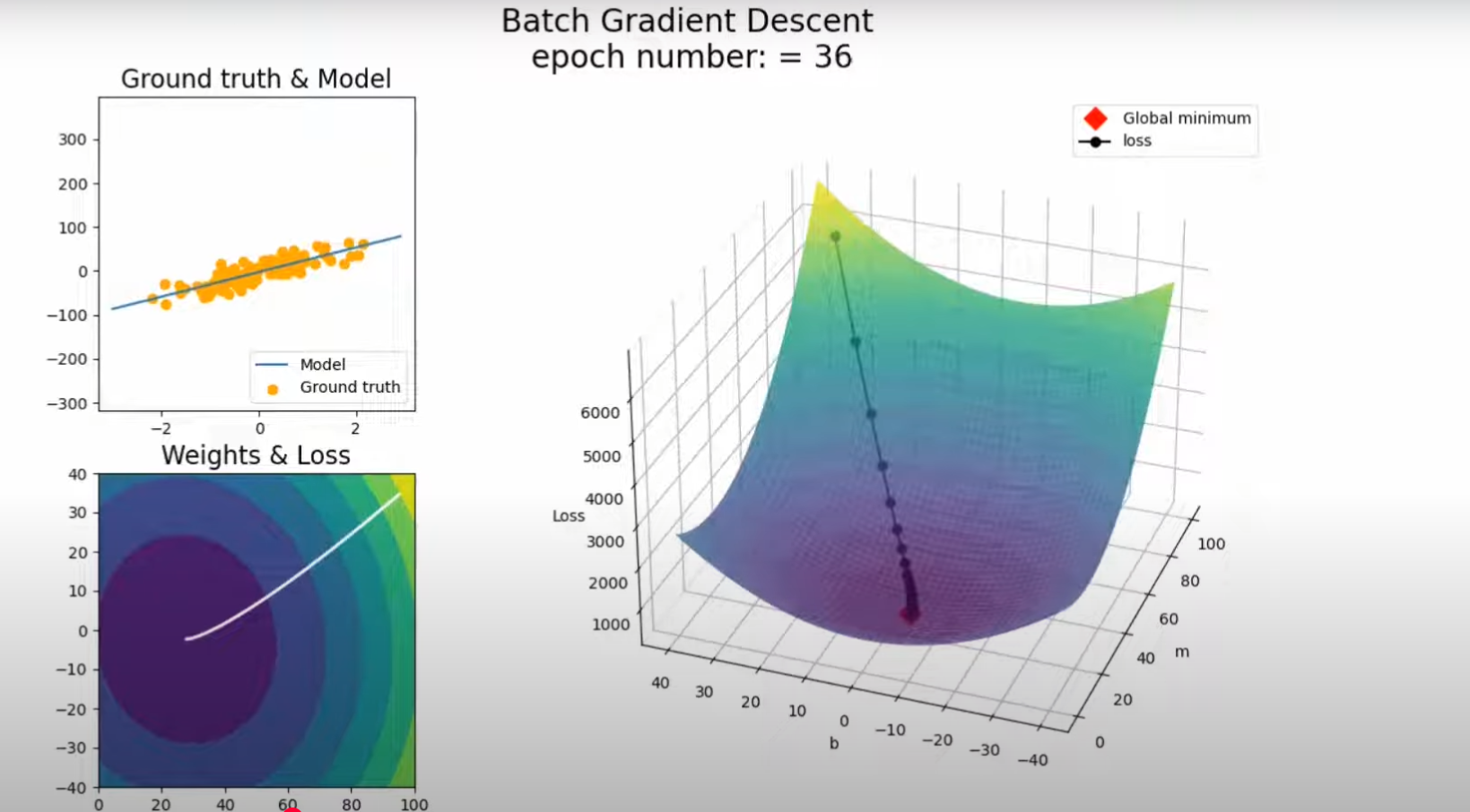
- Stochastic Gradient Descent: Optimizes with each sample instead of the entire dataset, which is faster but more noisy.
from tensorflow.keras.optimizers import SGD
optimizer = SGD(learning_rate=0.01)
- Momentum: Momentum helps accelerate SGD by moving along relevant directions and dampening oscillations. It adds a fraction of the previous update to the current one.
from tensorflow.keras.optimizers import SGD
optimizer = SGD(learning_rate=0.01, momentum=0.9)
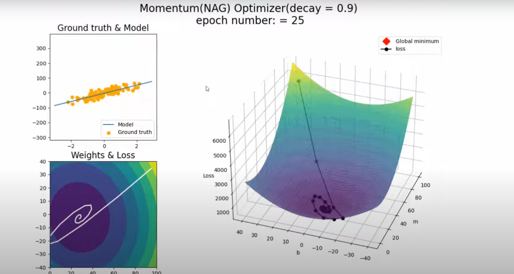
- NAG: An improvement over momentum. It looks ahead by calculating the gradient not just at the current position but slightly ahead, giving better convergence.
from tensorflow.keras.optimizers import SGD
optimizer = SGD(learning_rate=0.01, momentum=0.9, nesterov=True)
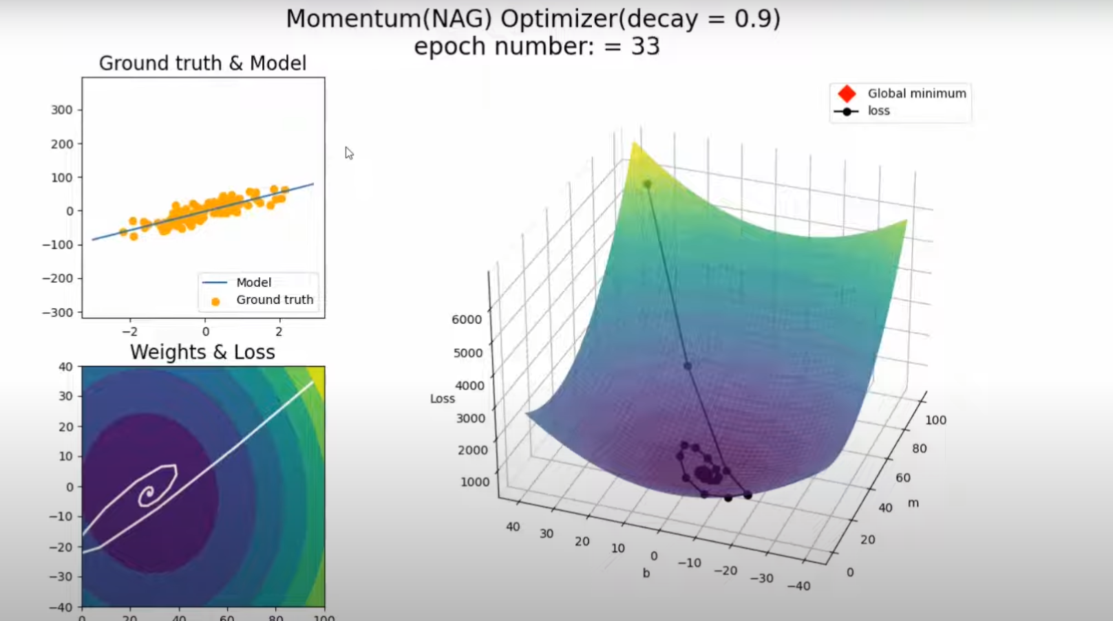
- AdaGrad: Adapts the learning rate to the parameters, performing larger updates for infrequent parameters and smaller updates for frequent ones.
from tensorflow.keras.optimizers import Adagrad
optimizer = Adagrad(learning_rate=0.01)
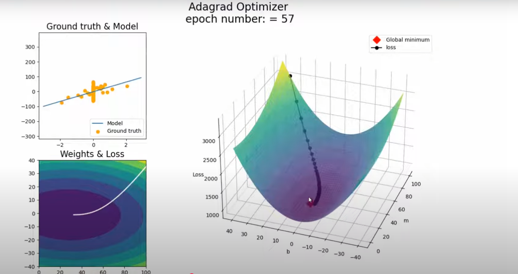
- RMSProp: Divides the learning rate by an exponentially decaying average of squared gradients. Useful for non-stationary objectives.
from tensorflow.keras.optimizers import RMSprop
optimizer = RMSprop(learning_rate=0.001)
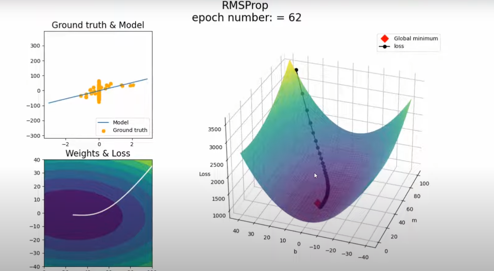
- ADAM (Adaptive Moment Estimation): Adaptive learning rate method that combines the advantages of RMSprop and momentum. Popular for its efficiency.
from tensorflow.keras.optimizers import Adam
optimizer = Adam(learning_rate=0.001)
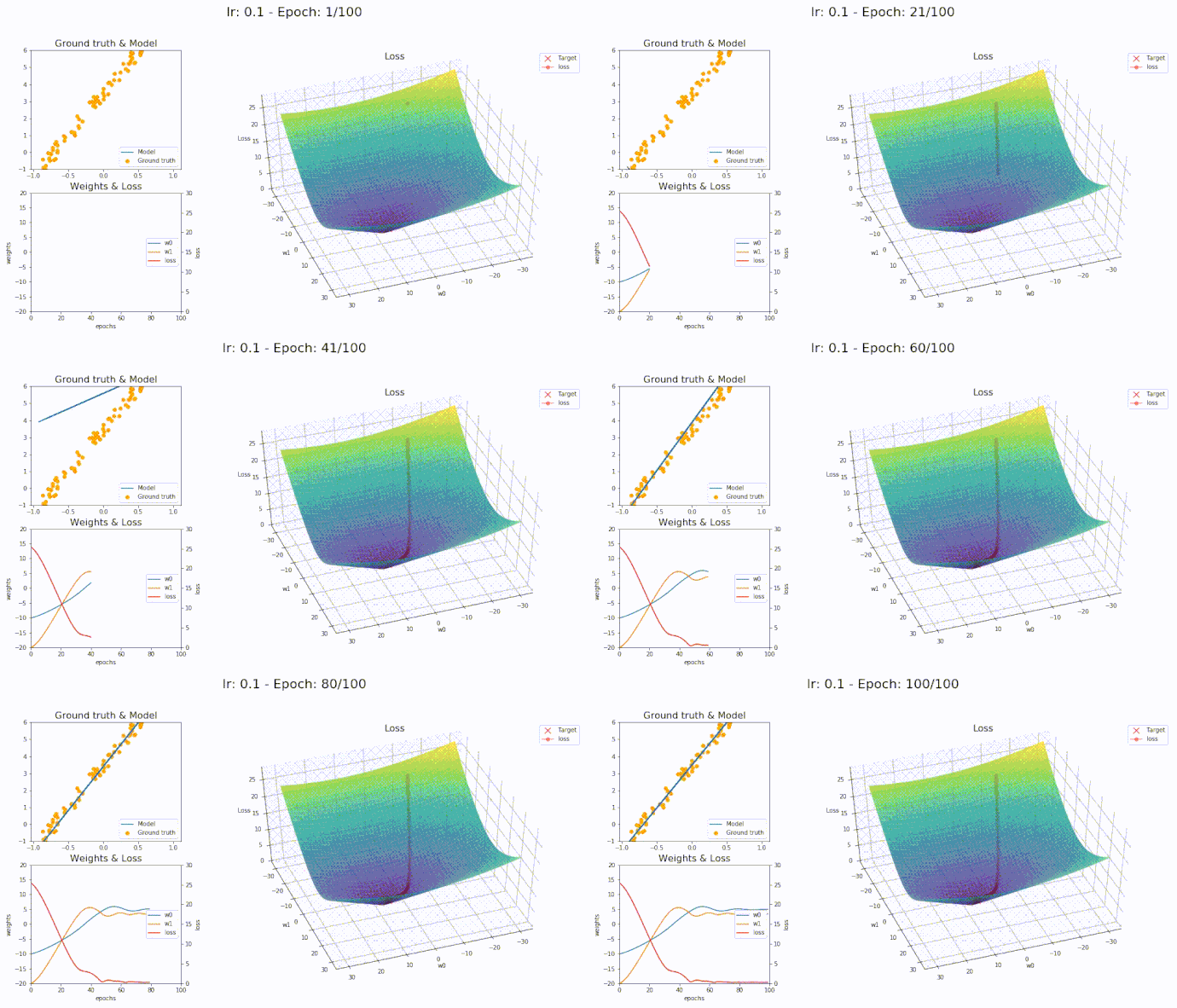
Overall:
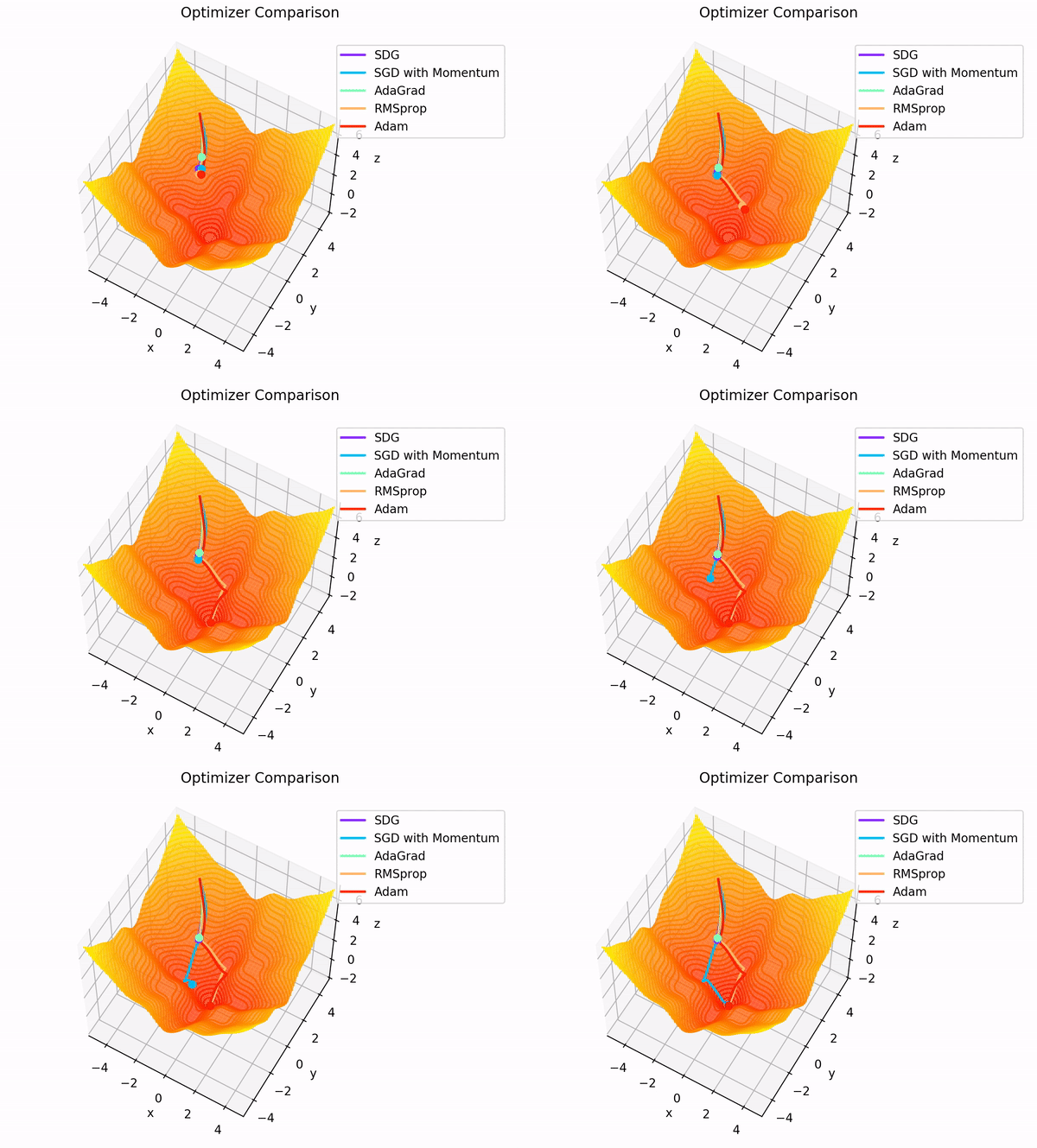 Notes:
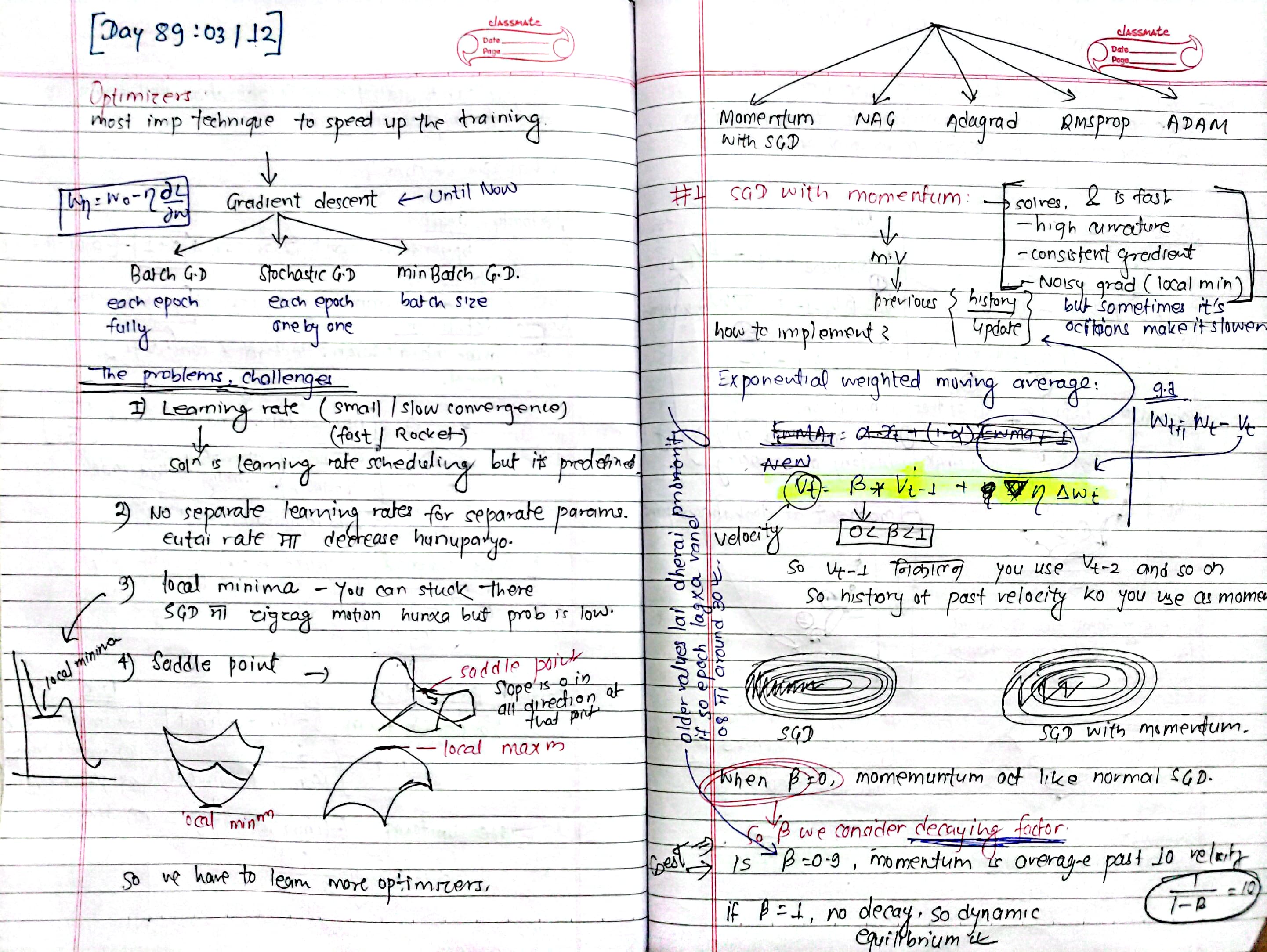
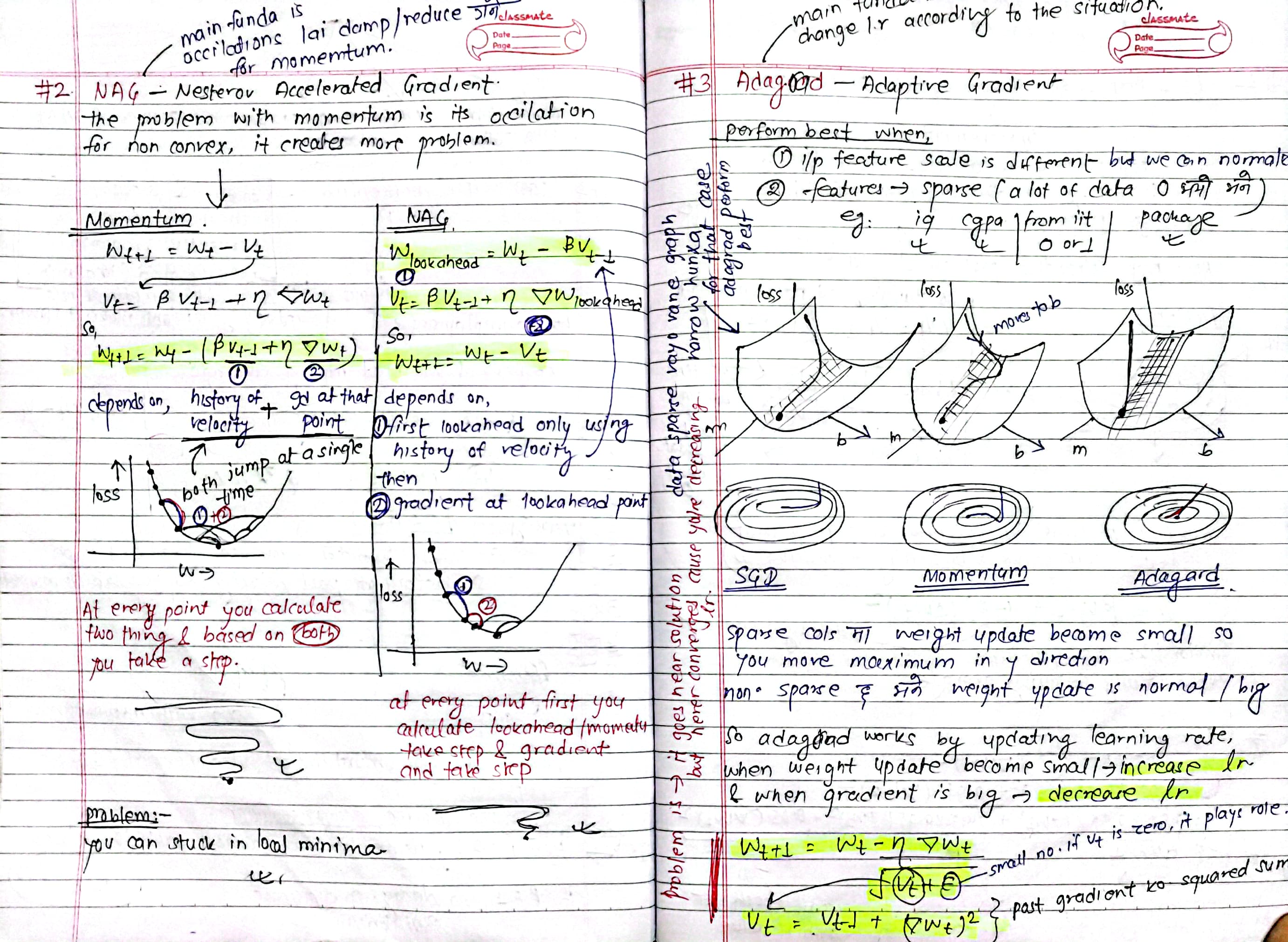
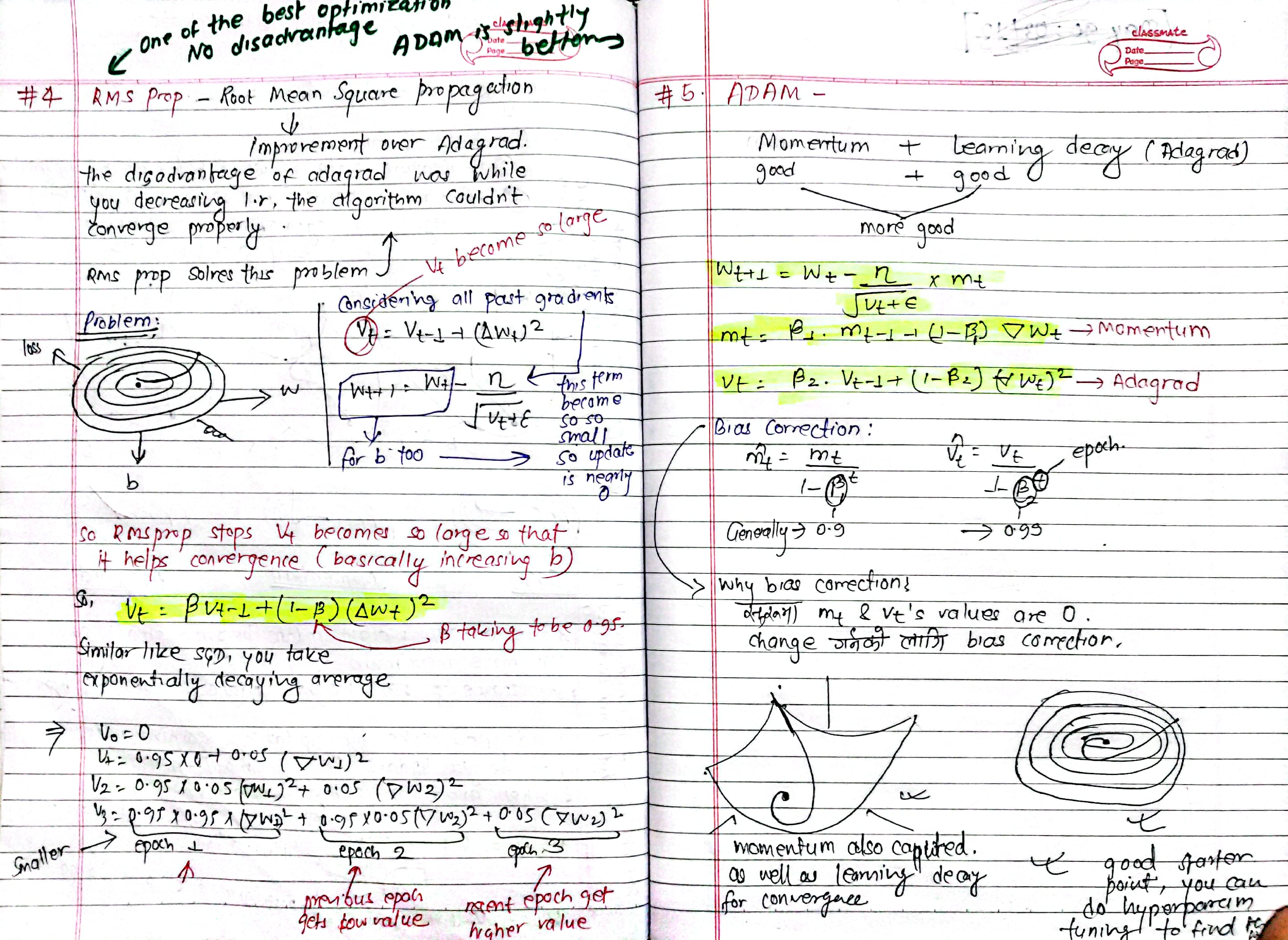
Interactive Visualization of Optimization Algorithms in Deep Learning: https://emiliendupont.github.io/2018/01/24/optimization-visualization/
Day 90: Keras Tuner
hyperparameters (like learning rate, batch size, optimizer) directly impact model performance. tuning helps optimize accuracy and generalization.
in my case, i worked with the diabetes dataset and focused on tuning key hyperparameters like learning rate, batch size, optimizer, number of neurons, and dropout rate. each of these parameters influences different aspects of training—for example, the learning rate affects how quickly the model converges, while dropout helps prevent overfitting.
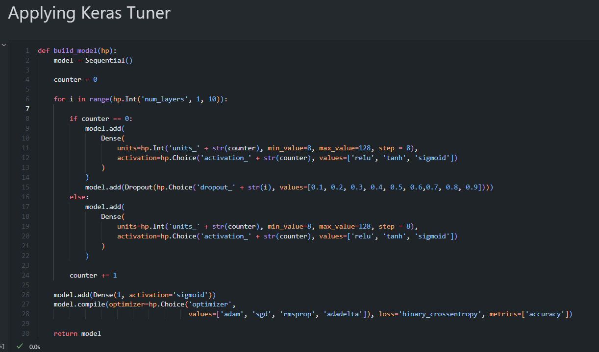
to streamline the tuning process, i used keras tuner’s RandomSearch. i defined a hypermodel where parameters like the number of layers, neurons, dropout rates, learning rates, and optimizer types were set as tunable. the objective was to maximize validation accuracy. i also configured settings like max_trials to control the search space and executions_per_trial to ensure consistent evaluation.
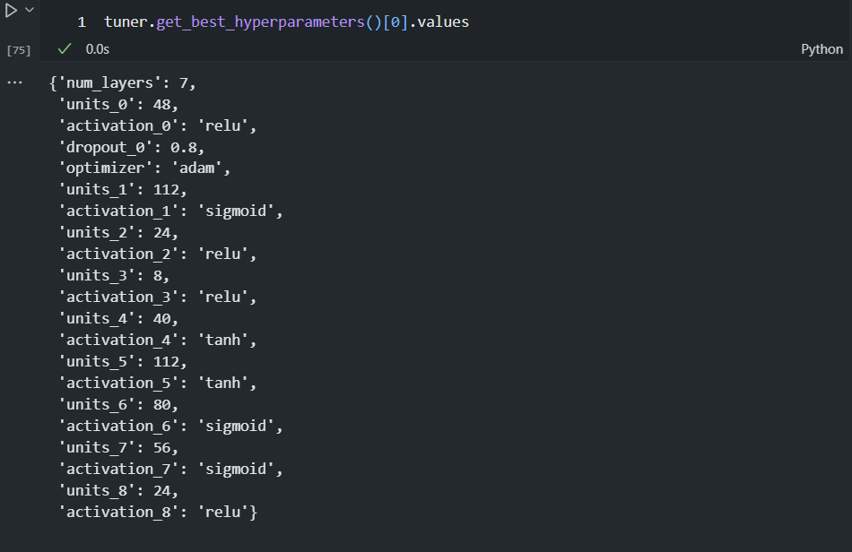
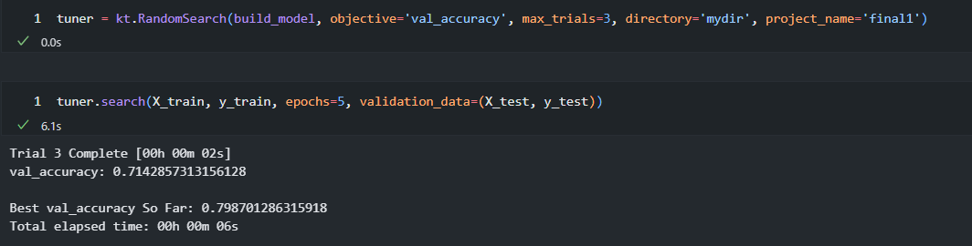 after running the tuning process, the model achieved around 79% accuracy. the tuning helped balance model complexity and performance, reducing overfitting and improving generalization.
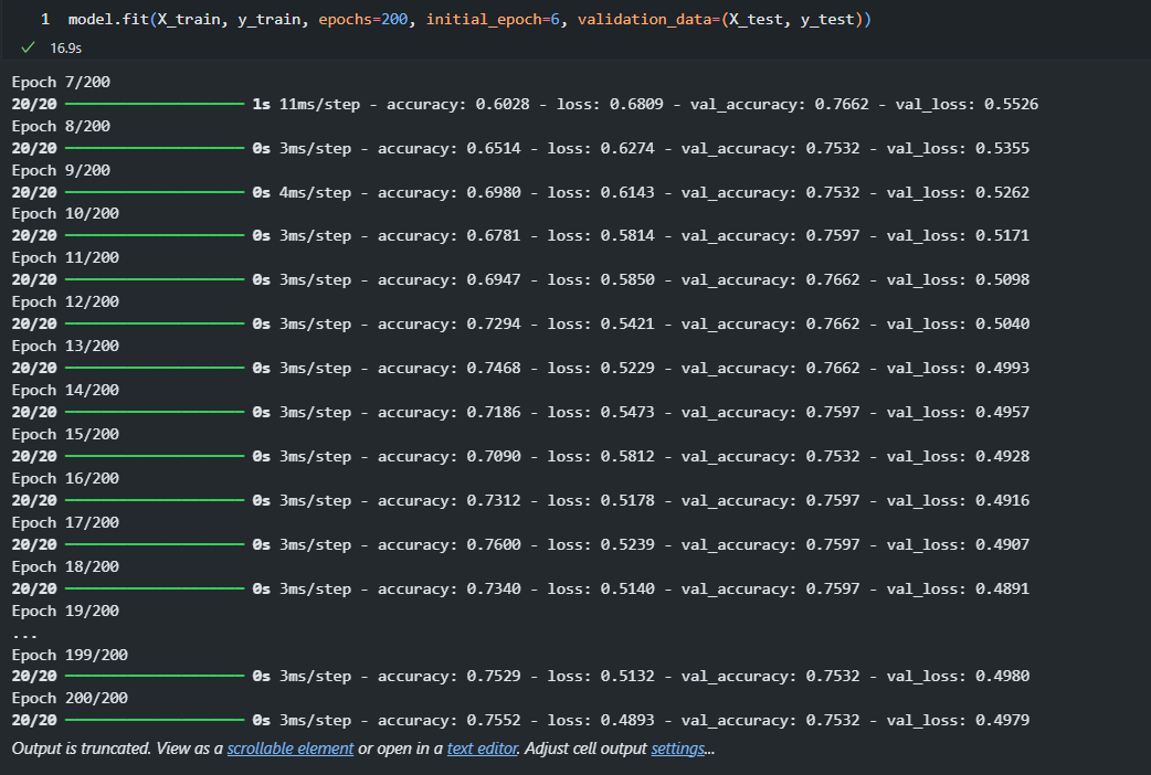 for further improvements, i could fine-tune hyperparameters like the learning rate and dropout in smaller increments, try advanced optimizers like adamw, or implement early stopping to avoid unnecessary training once the model stops improving.
Day 91: Deep Diving into CNNs:
Focused on planning a deep dive into cnns. explored why anns fall short for cnn tasks and uncovered some fascinating cnn applications. along the way, stumbled upon some surprisingly cool ideas for future projects. fueled by that curiosity, i tried something basic today—simple, but a solid starting point.
today, i explored opencv from scratch, debugged image loading issues, applied basic filters using custom convolution kernels in pure python as well as with Opencv, and created amazingly undefinable custom filters with the excitement.
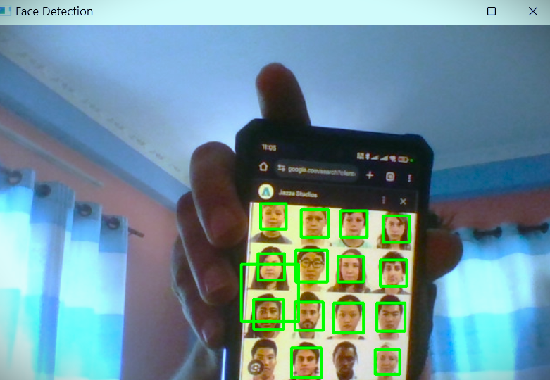 Notebook:Trying OpenCV for the first time
Watch out notebook what i did with this lovely image:
Notebook:Trying OpenCV for the first time
Watch out notebook what i did with this lovely image:

Notes:
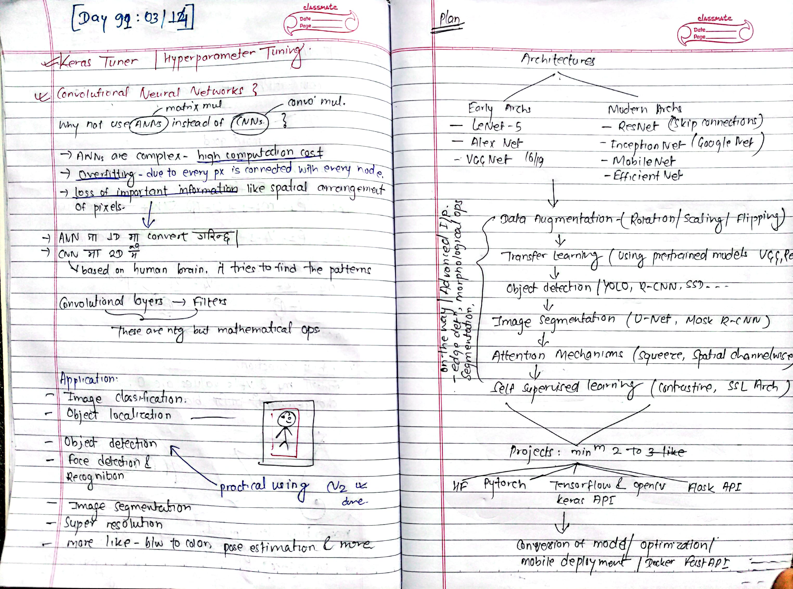
architectures
- early arch
- lenet-5
- alexnet
- vgg net (16/19)
- modern arch
- resnet (skip connection)
- inception net (google net)
- mobilenet
- efficientnet
Plan after Architecture
- data augmentation (rotation, scaling, flipping)
- transfer learning (using pretrained models like vgg, resnet)
- object detection (yolo, r-cnn, ssd, etc.)
- image segmentation (u-net, mask r-cnn)
- attention mechanisms (squeeze, spatial channel-wise)
- self-supervised learning (contrastive, ssl architectures)
Day 92: Understanding Paddings and Strides
How CNNs working with Grayscale and Rgb images??
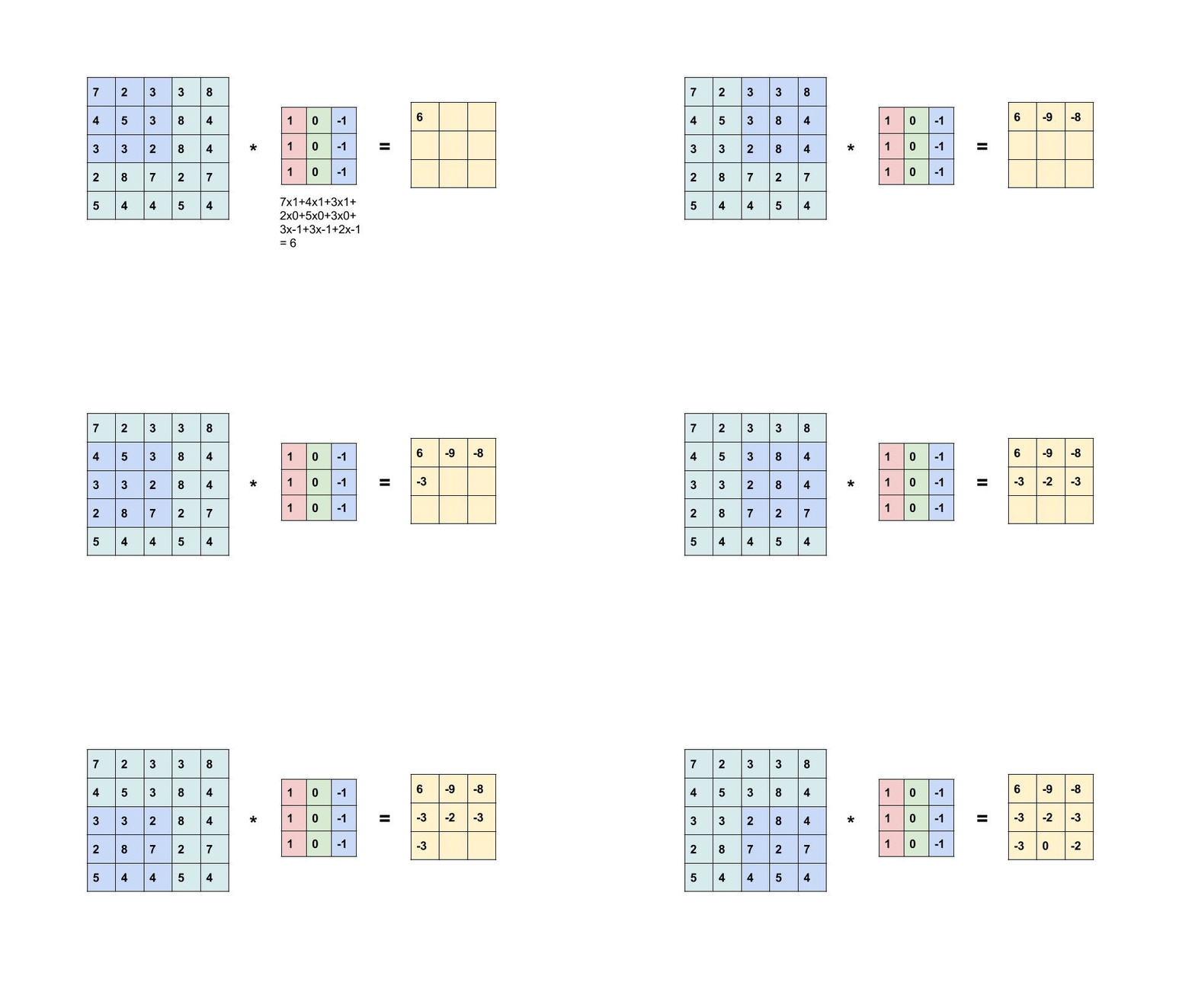
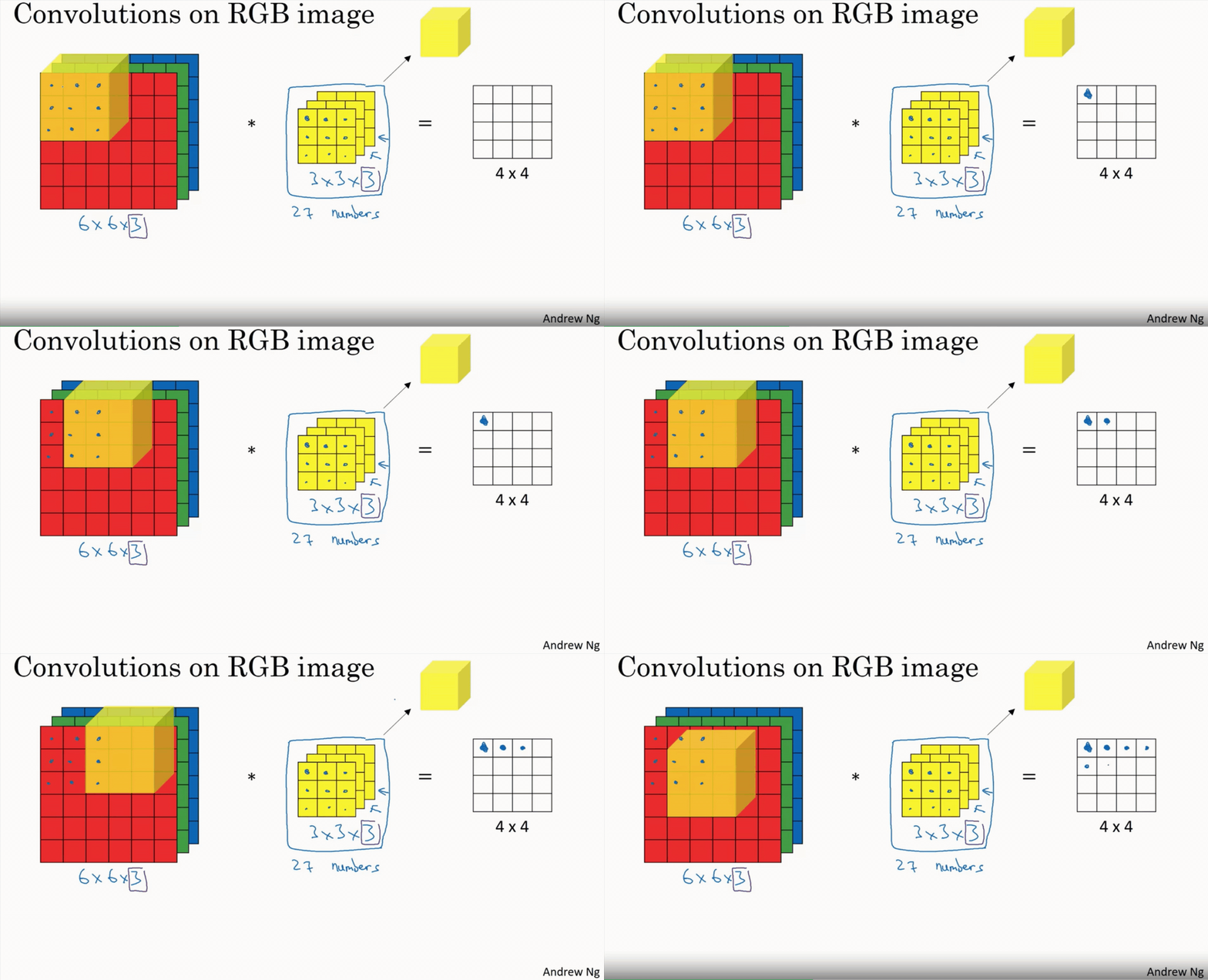
padding and strides are important in convolutional neural networks (cnns) because they affect feature extraction, output size, and computational efficiency.
Padding is used to prevent reduction in spatial dimensions and retain edge information. for example, a 5x5 image with a 3x3 filter produces a 3x3 feature map, which keeps shrinking with more layers. adding padding helps maintain the size.
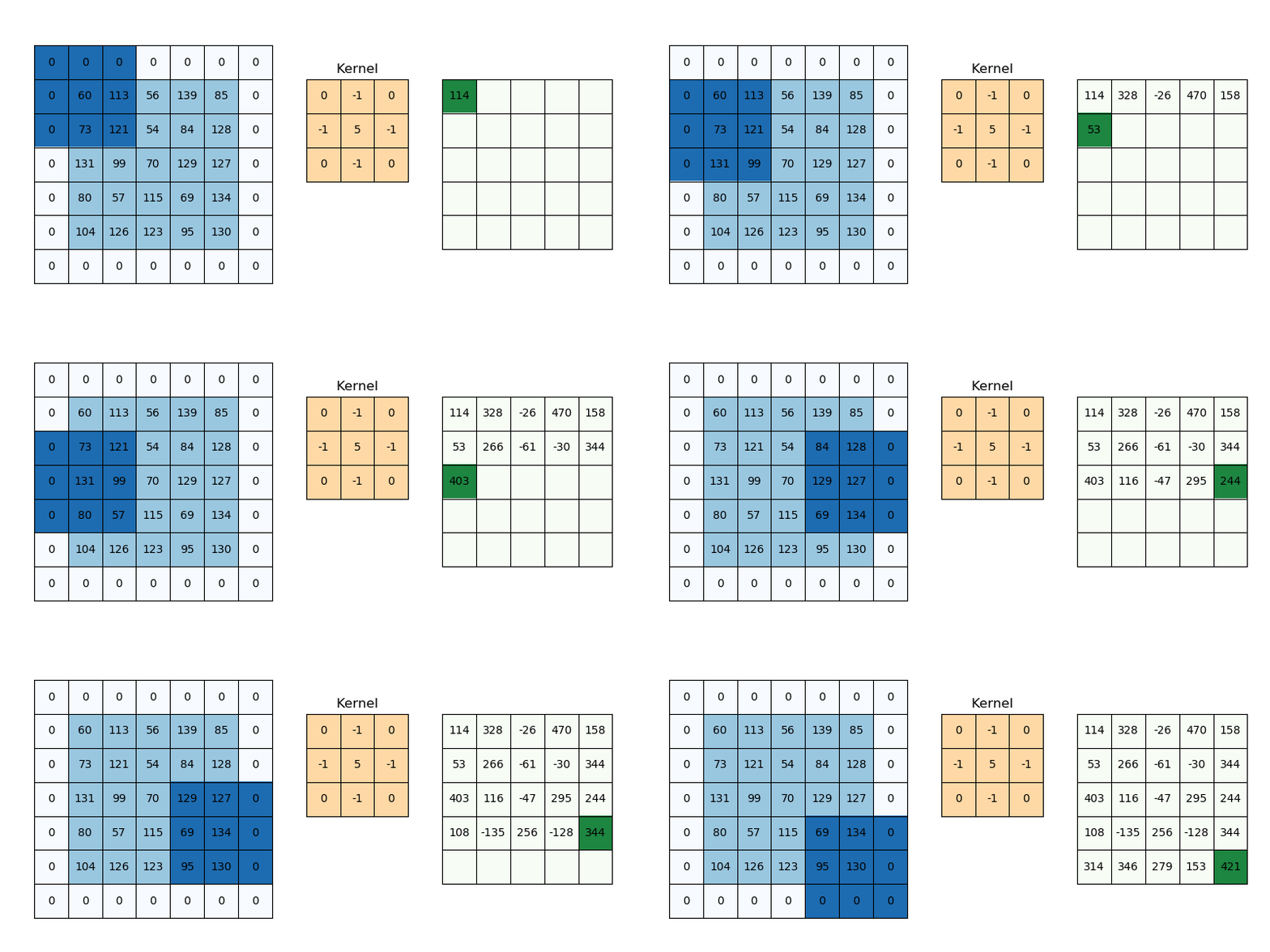 there are two common types of padding:
- valid: no padding, meaning the output size shrinks.
- same: pads the input so the output size remains the same.
the output size with padding is calculated as:
(n + 2p - f + 1) × (n + 2p - f + 1), where n is the input size, f is the filter size, and p is the padding amount.
in keras, padding is applied like this Demo for MNIST:
# Importing necessary libraries
import tensorflow as tf
from tensorflow.keras.layers import Dense, Conv2D, Flatten
from tensorflow.keras.models import Sequential
from tensorflow.keras.datasets import mnist

# Loading MNIST dataset
(X_train, y_train), (X_test, y_test) = mnist.load_data()

# Creating a Sequential model
model = Sequential()

# Adding Convolutional layers with valid padding
model.add(Conv2D(32, kernel_size=(3,3), padding='valid', activation='relu', input_shape=(28,28,1)))
model.add(Conv2D(32, kernel_size=(3,3), padding='valid', activation='relu'))
model.add(Conv2D(32, kernel_size=(3,3), padding='valid', activation='relu'))

model.add(Flatten())

model.add(Dense(128, activation='relu'))
model.add(Dense(10, activation='softmax'))

# Printing model summary
model.summary()
strides control how far the filter moves across the image at each step. a stride of (1,1) moves one pixel at a time, while higher strides skip pixels, reducing spatial dimensions and computation time.
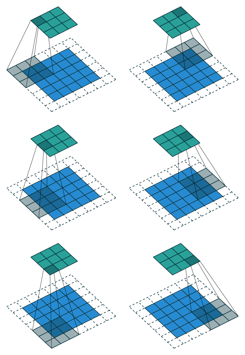 output size with strides is calculated as:
((n + 2p - f) / s + 1) × ((n + 2p - f) / s + 1), where s is the stride value.
higher strides help capture larger patterns but reduce spatial resolution. for example, a stride of (2,2) makes the filter shift 2 pixels at a time:
# Importing necessary libraries
import tensorflow as tf
from tensorflow.keras.layers import Dense, Conv2D, Flatten
from tensorflow.keras.models import Sequential
from tensorflow.keras.datasets import mnist

# Loading MNIST dataset
(X_train, y_train), (X_test, y_test) = mnist.load_data()

# Creating a Sequential model with strides
model = Sequential()

model.add(Conv2D(32, kernel_size=(3,3), padding='same', strides=(2,2), activation='relu', input_shape=(28,28,1)))
model.add(Conv2D(32, kernel_size=(3,3), padding='same', strides=(2,2), activation='relu'))
model.add(Conv2D(32, kernel_size=(3,3), padding='same', strides=(2,2), activation='relu'))

model.add(Flatten())

model.add(Dense(128, activation='relu'))
model.add(Dense(10, activation='softmax'))

# Printing model summary
model.summary()
in summary, padding helps retain image details and control output size, while strides affect computational efficiency and feature abstraction. tuning these parameters is key to optimizing cnns.
Pooling:
pooling is used to downsample feature maps, reducing their size while retaining important information. it helps prevent overfitting and reduces computation.
common types of pooling:
 max pooling: selects the maximum value in a region.
average pooling: takes the average of values in a region.
for example, a 2x2 max pooling layer with stride 2 reduces feature maps to half their original size.
max pooling: selects the maximum value in a region.
average pooling: takes the average of values in a region.
for example, a 2x2 max pooling layer with stride 2 reduces feature maps to half their original size.
# importing necessary libraries
import tensorflow as tf
from tensorflow.keras.layers import Dense, Conv2D, Flatten, MaxPooling2D
from tensorflow.keras.models import Sequential
from tensorflow.keras.datasets import mnist

# loading mnist dataset
(X_train, y_train), (X_test, y_test) = mnist.load_data()

# reshaping input data
X_train = X_train.reshape(-1, 28, 28, 1).astype('float32') / 255
X_test = X_test.reshape(-1, 28, 28, 1).astype('float32') / 255

# creating a sequential model
model = Sequential()

# adding convolutional layers with padding
model.add(Conv2D(32, kernel_size=(3,3), padding='same', activation='relu', input_shape=(28,28,1)))
model.add(MaxPooling2D(pool_size=(2,2), strides=(2,2)))

model.add(Conv2D(64, kernel_size=(3,3), padding='same', activation='relu'))
model.add(MaxPooling2D(pool_size=(2,2), strides=(2,2)))

model.add(Conv2D(128, kernel_size=(3,3), padding='same', activation='relu'))
model.add(MaxPooling2D(pool_size=(2,2), strides=(2,2)))

# flattening and adding dense layers
model.add(Flatten())
model.add(Dense(128, activation='relu'))
model.add(Dense(10, activation='softmax'))

# printing model summary
model.summary()
Day 93: Backpropagation in cnns: a quick breakdown
cnns learn by adjusting their parameters through backpropagation. here's how:
- forward propagation:
- input passes through convolution → relu → max pooling → flatten → fully connected layers → output.
- backpropagation:
- calculate loss and propagate errors backward.
- use the chain rule to compute gradients for weights, biases, and activations.
- layer-wise backprop:
- convolutional layers: errors backpropagate through filters.
- max pooling: only max-selected neurons contribute gradients.
- flattening: reshapes gradients before sending them back.
Notes:
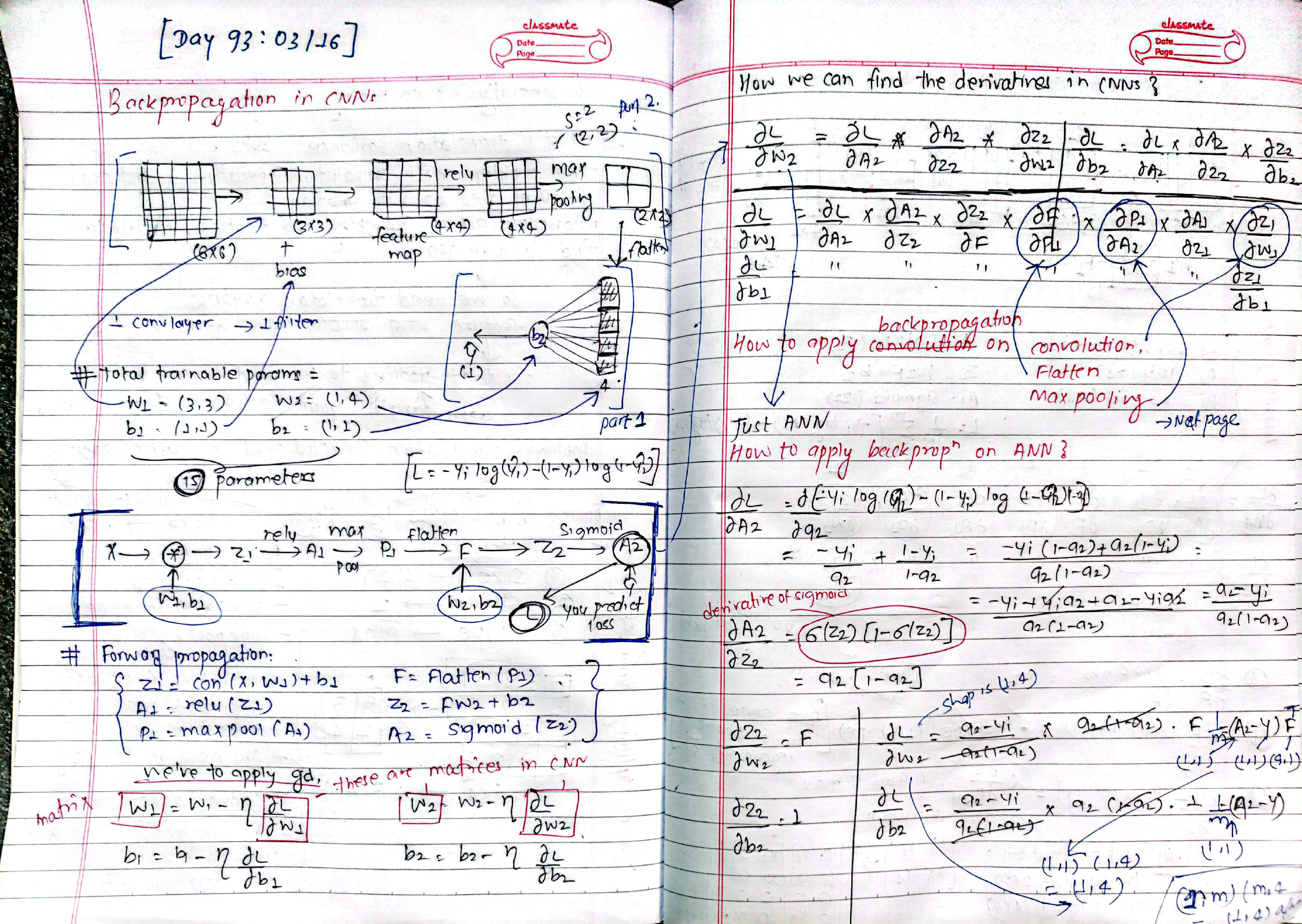
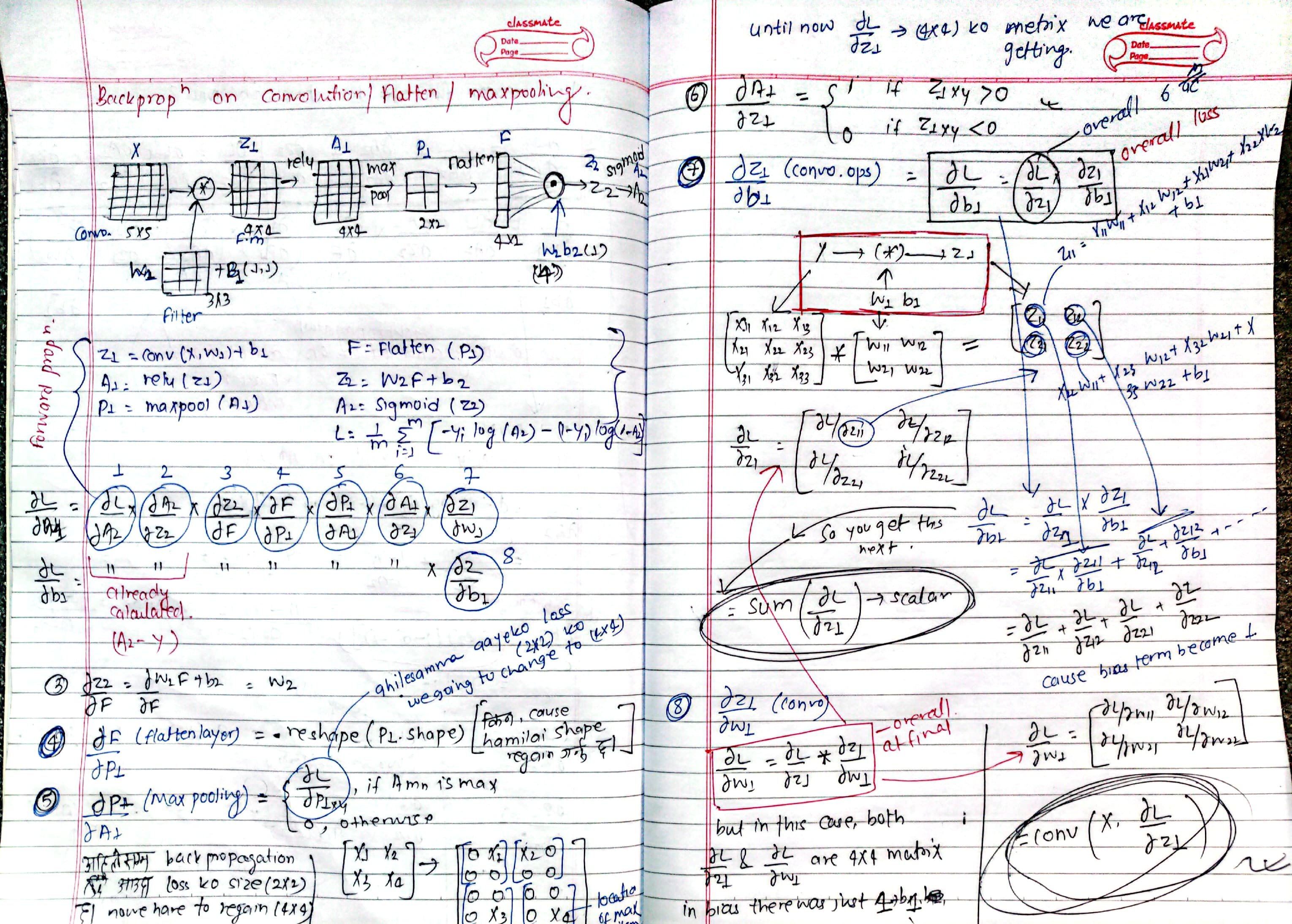
Day 94: LeNet5, Cat Vs Dog Classification
LeNet-5, introduced by Yann LeCun in 1989, is one of the earliest convolutional neural networks (CNNs), designed for handwritten character recognition. It consists of seven layers:
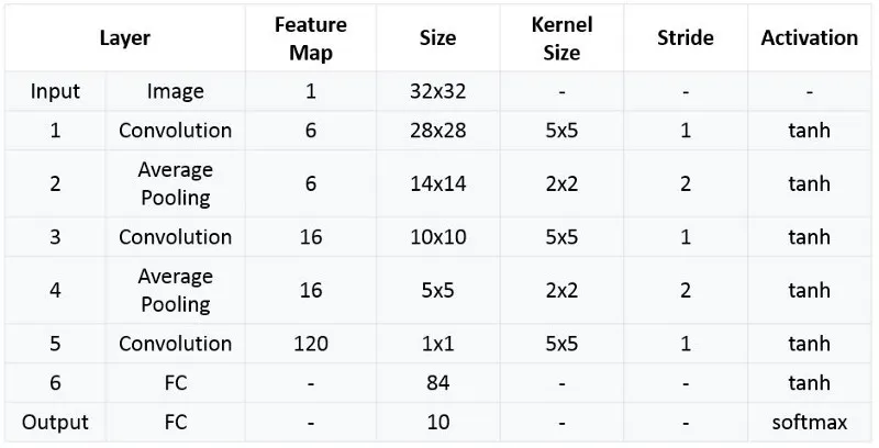
- Input Layer: 32×32 grayscale image.
- Conv Layer 1 (C1): 6 filters (5×5), output size 28×28×6.
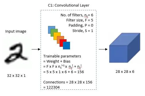
- Pooling Layer 1 (S2): Average pooling (2×2), output 14×14×6.
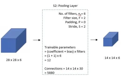
- Conv Layer 2 (C3): 16 filters (5×5), selectively connected, output 10×10×16.
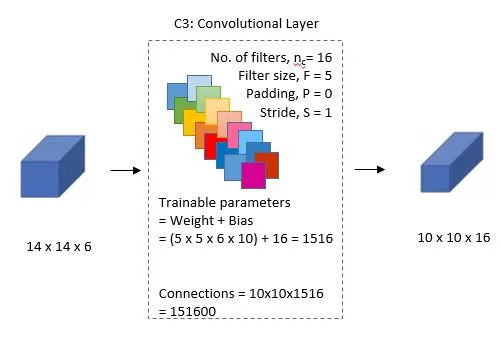
- Pooling Layer 2 (S4): Average pooling (2×2), output 5×5×16.
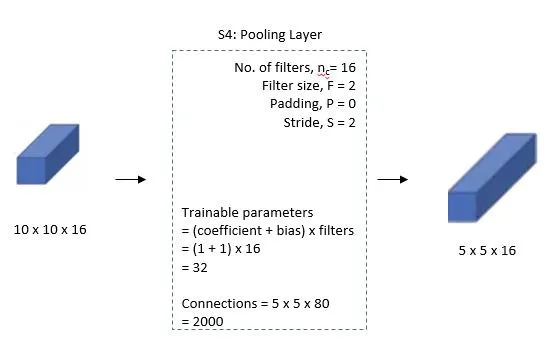
- Fully Connected (C5): 120 neurons, connected to all 5×5×16 inputs.
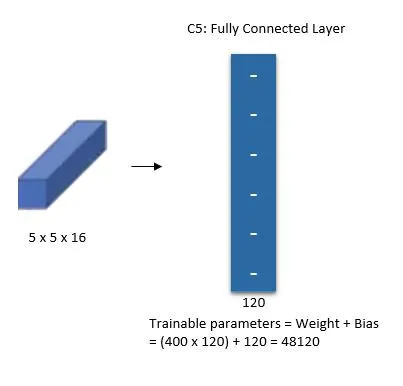
- Fully Connected (F6): 84 neurons.
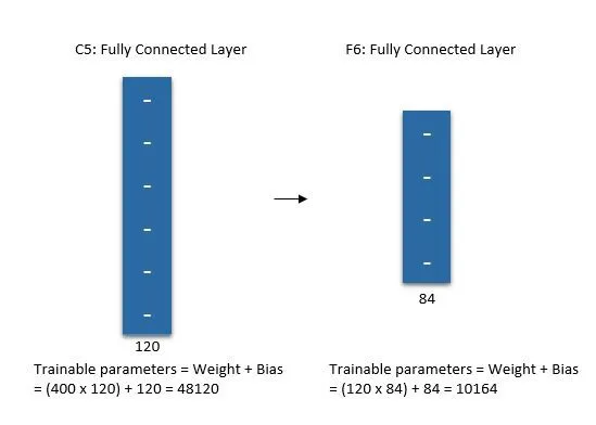
- Output Layer: Softmax with 10 classes (digits 0-9).
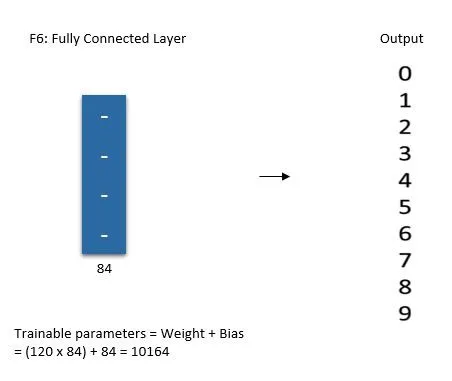
Implementation:
def build_lenet(input_shape):
  # Define Sequential Model
  model = tf.keras.Sequential()

  # C1 Convolution Layer
  model.add(tf.keras.layers.Conv2D(filters=6, strides=(1,1), kernel_size=(5,5), activation='tanh', input_shape=input_shape))

  # S2 SubSampling Layer
  model.add(tf.keras.layers.AveragePooling2D(pool_size=(2,2), strides=(2,2)))

  # C3 Convolution Layer
  model.add(tf.keras.layers.Conv2D(filters=6, strides=(1,1), kernel_size=(5,5), activation='tanh'))

  # S4 SubSampling Layer
  model.add(tf.keras.layers.AveragePooling2D(pool_size=(2,2), strides=(2,2)))

  # C5 Fully Connected Layer
  model.add(tf.keras.layers.Dense(units=120, activation='tanh'))

  # Flatten the output so that we can connect it with the fully connected layers by converting it into a 1D Array
  model.add(tf.keras.layers.Flatten())

  # FC6 Fully Connected Layers
  model.add(tf.keras.layers.Dense(units=84, activation='tanh'))

  # Output Layer
  model.add(tf.keras.layers.Dense(units=10, activation='softmax'))

  # Compile the Model
  model.compile(loss='categorical_crossentropy', optimizer=tf.keras.optimizers.SGD(lr=0.1, momentum=0.0, decay=0.0), metrics=['accuracy'])

  return model
Day 95: GPU slow than CPU - well in my case?
Today, I trained an MNIST model on both CPU (Ryzen 7 6000) and GPU (RTX 3050 Ti), expecting a significant speedup with the GPU. Instead, the CPU performed slightly faster, and when I tried adding a small CNN, my GPU environment crashed, while the CPU handled it fine (but slower).
- The GPU initially took longer due to kernel warm up and data transfer overhead.
- Batch Size Impact – GPUs perform best with larger batch sizes (e.g., 512+), while I used a smaller batch.
- Data Bottlenecks – My CPU handled data preloading better, while the GPU might have suffered from inefficient memory access.
- GPU Utilization – The GPU wasn’t fully utilized, likely due to suboptimal parallelism in my setup.
And When I added even a small convo layer, my GPU environment crashed, but the CPU ran it (slowly). here’s what possible reason i estimated?
- My RTX 3050 Ti has 4GB VRAM, and it might be running out.
- Despite setting up a dedicated GPU environment (with proper CUDA, cuDNN, and TensorFlow versions), I couldn’t debug this issue today.
- There might be a compatibility issue between TensorFlow, CUDA, and my system's architecture.
Could it be a CUDA/cuDNN issue or VRAM exhaustion?
I used two separate virtual environments:
- CPU environment (normal setup)
- GPU environment (proper versions of CUDA, TensorFlow, and cuDNN) Still, I couldn’t debug the crashes today. Any suggestions on debugging the bit architecture issue or possible TensorFlow config problems? and is it abnormal CPU performing better than GPU in my optimization??
Here's the comparision:
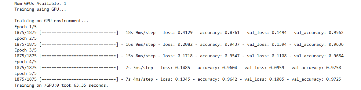
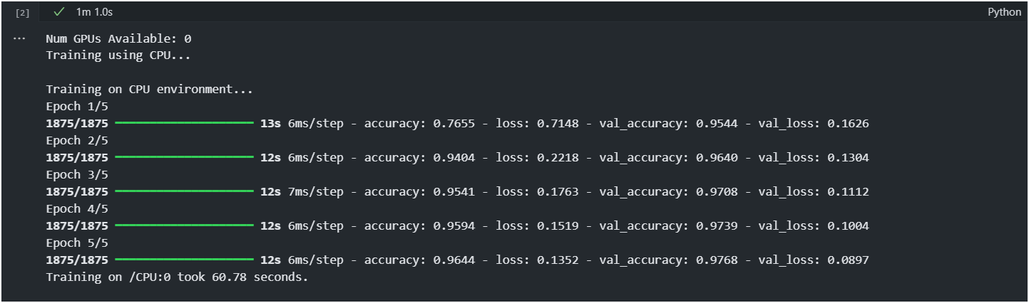
Some rough notebooks: Notebook: CPU Notebook: GPU
Day 96: Data Augmentation, Pretrained Models
Data augmentation is crucial in machine learning, especially for tasks like computer vision, to enhance model performance and prevent overfitting. It involves applying various transformations to existing data, such as rotation, translation, scaling, flipping, shearing, zooming, and adjusting brightness and contrast. These techniques help in creating a larger and more diverse training dataset, thereby improving model generalization.
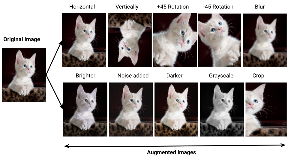
Why Use Data Augmentation?
- Increased Dataset Size: Enhances model training with more examples.
- Regularization: Adds noise to prevent overfitting.
- Improved Generalization: Helps models perform better on unseen data.
Notebook: data augmentation on cifar10 frog
Pretrained models in CNN:
Notes:
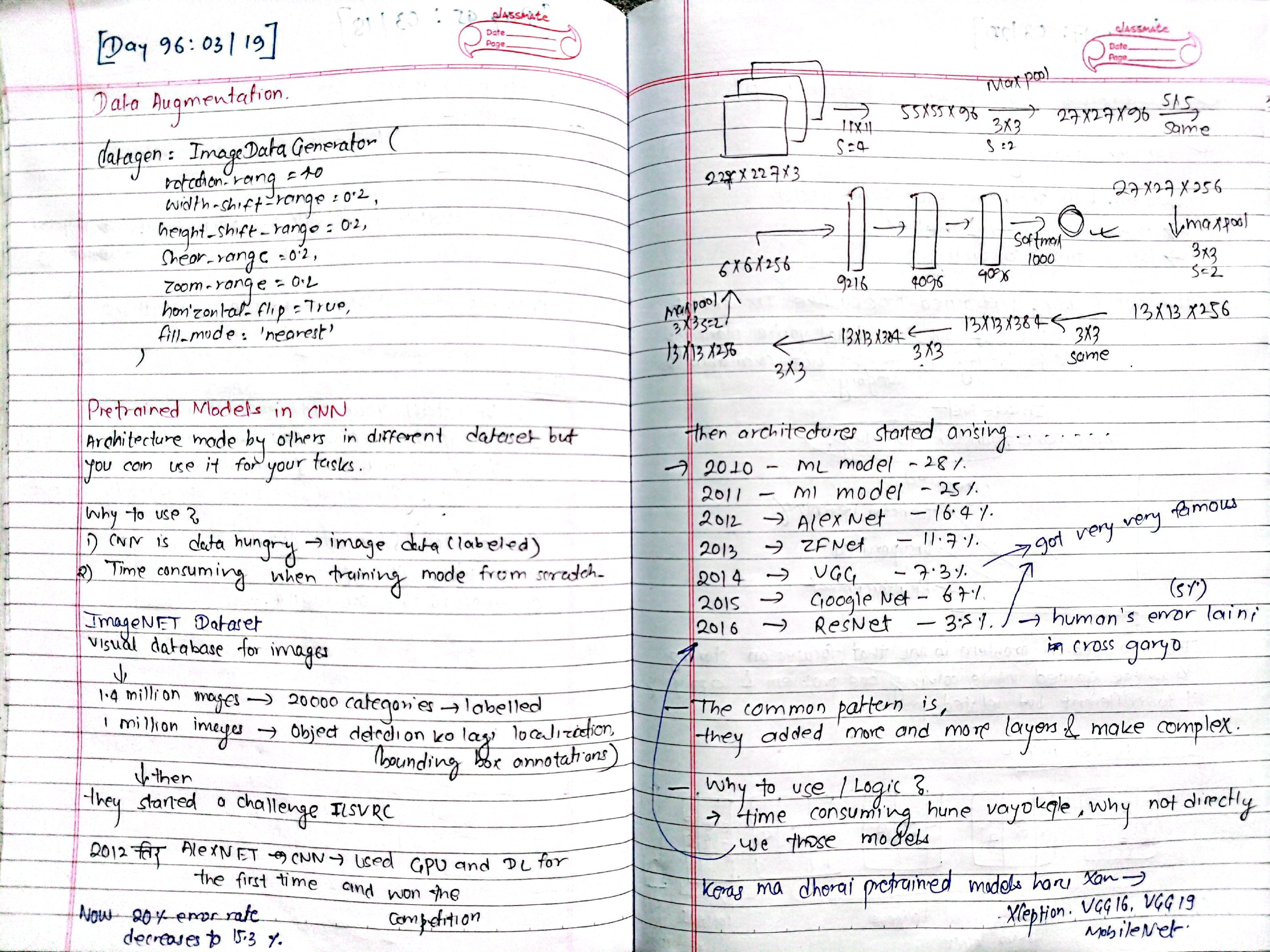
before deep learning took over, imagenet models relied on classical ml methods like svm, decision trees, and hand-crafted features (think hog, sift, and lbp). this worked, but scaling to millions of images? a nightmare. then alexnet (2012) happened—deep cnns trained with relu activations and dropout on gpus. it crushed traditional methods, slashing classification error rates by half.
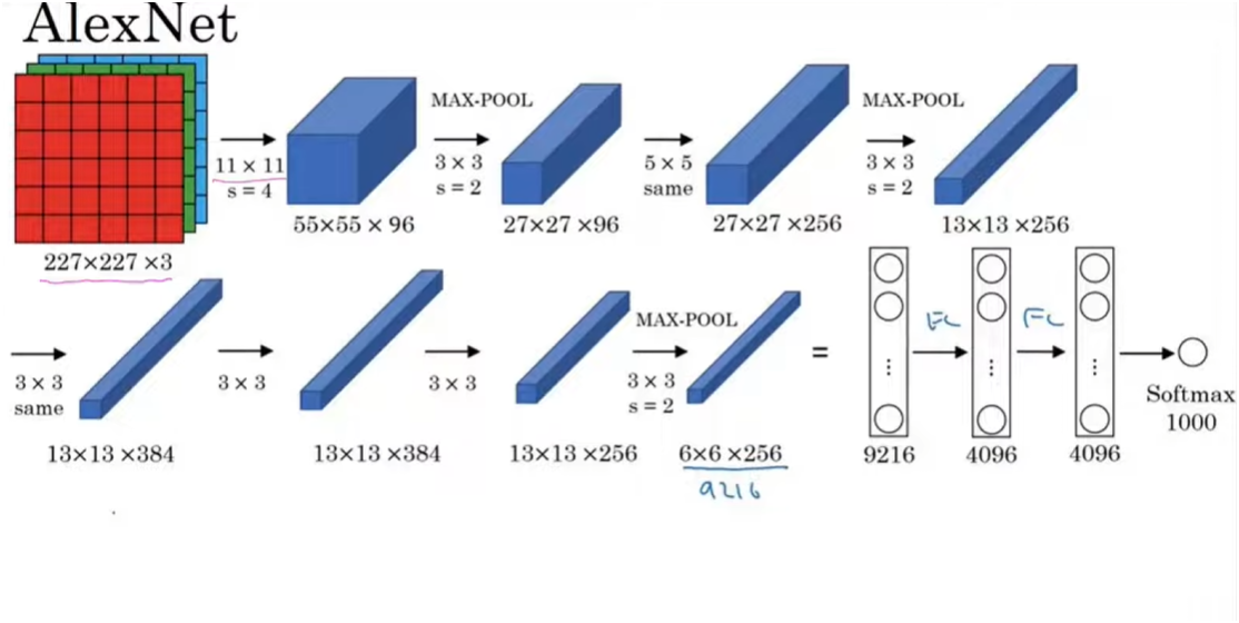
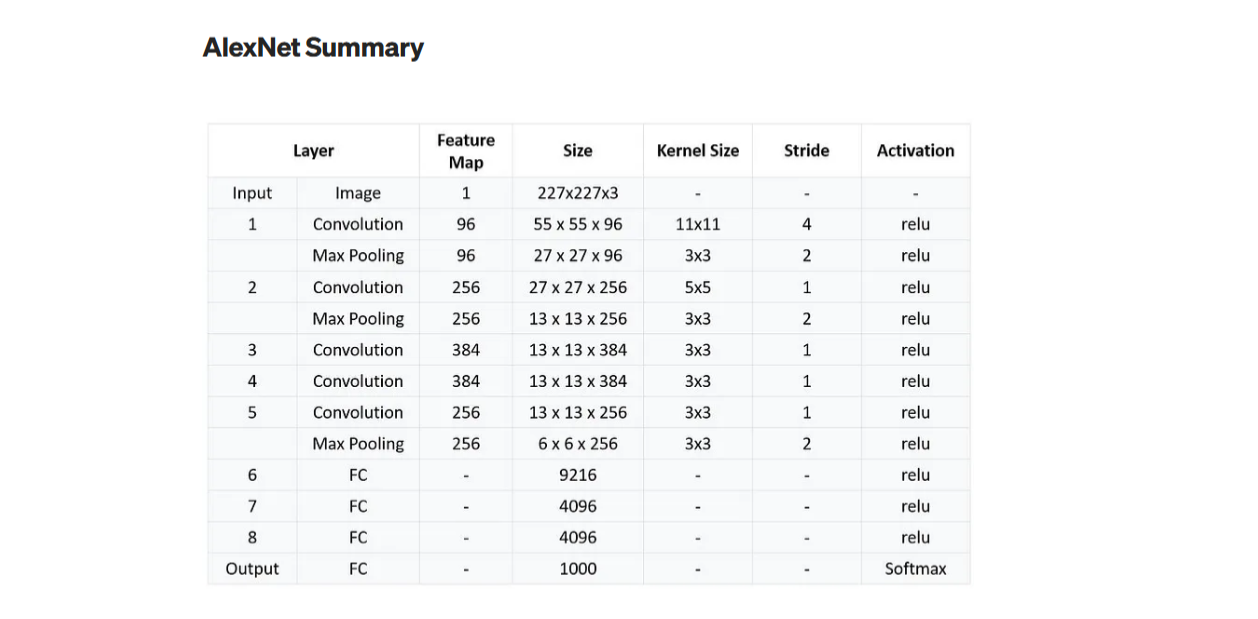
vgg (2014) pushed deeper with 3x3 convolutions, proving that simplicity + depth = power. same year, googlenet (inception v1) introduced inception modules—parallel conv layers reducing parameter overhead while boosting efficiency. resnet (2015) then solved the vanishing gradient problem with skip connections, making ultra-deep networks (152 layers!) trainable.
today, pretrained models built on imagenet—resnet, vgg, inception, efficientnet—are the backbone of modern deep learning. explored these today, and yeah, standing on the shoulders of giants makes life easier.
PaperLink: ImageNet Classification with Deep Convolutional Neural Networks
Keras pretrained models: https://keras.io/api/applications/
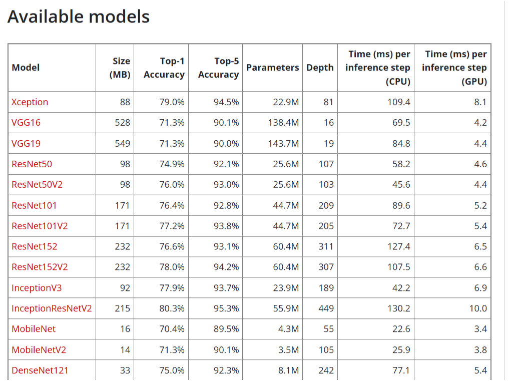
I will test the examples from that website using their code there in following notebook: Notebook: Pretrained Model Testing
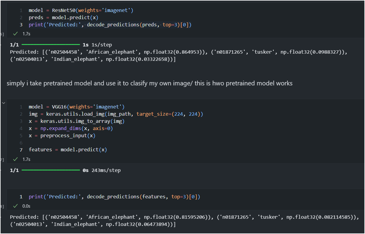
Day 97: Visualizing Convolutional Layers, Transfer learning
Today, i'll be using the article : https://machinelearningmastery.com/how-to-visualize-filters-and-feature-maps-in-convolutional-neural-networks/ with respect to following topics.
- Visualizing Convolutional Layers
- Pre-fit VGG Model
- How to Visualize Filters
- How to Visualize Feature Maps
Notebook: visualizing Layers with elephant image
notes:
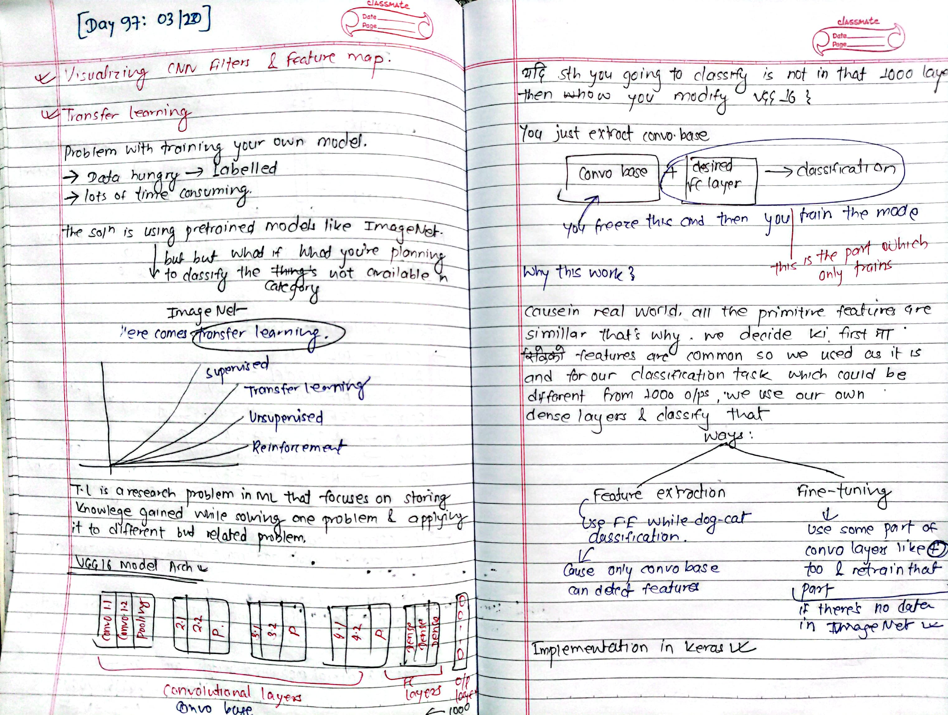
Transfer learning:
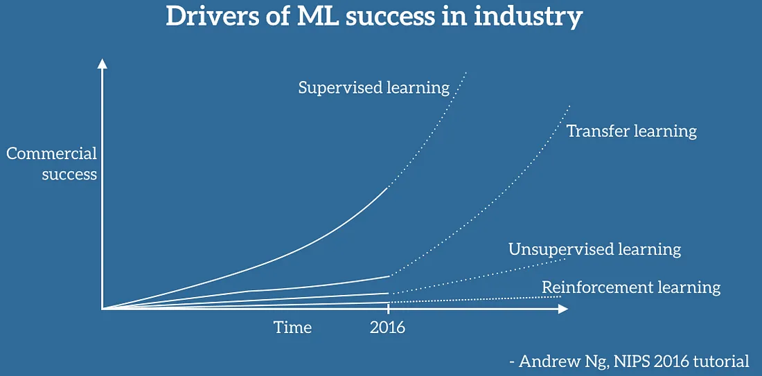 transfer learning helps train deep learning models efficiently by leveraging pre-trained networks like vgg, resnet, or mobilenet. instead of starting from scratch, we use the convolutional base (which extracts features) and replace the fully connected layers with our own classifier.
two main approaches:
- feature extraction – freeze the convolutional layers and train only the new classifier. useful when the target dataset is similar to the original dataset.
- fine-tuning – unfreeze some deeper layers and retrain them along with the classifier. this helps when the target dataset is quite different.
Resource: https://www.tensorflow.org/tutorials/images/transfer_learning
Day 98: Keras functional API
How to use keras functional api for deep learning?
Today i went through an article: https://machinelearningmastery.com/keras-functional-api-deep-learning/
The Sequential model API is great for developing deep learning models in most situations, but it also has some limitations.
I started with the Sequential API to build familiarity:
- Architecture: Simple CNN with
Conv2D → MaxPooling → Flatten → Dense → Output. - Workflow:
-
Loaded data, normalized pixels (
0-1), reshaped images (28x28x1), and one-hot encoded labels. -
Built a linear stack of layers:
model = Sequential([ Conv2D(32, (3,3), MaxPooling2D(), Flatten(), Dense(128), Dense(10, activation='softmax') ]) -
Trained with
model.fit(), achieving ~91% validation accuracy in 10 epochs.
-
2. Transition to Functional API
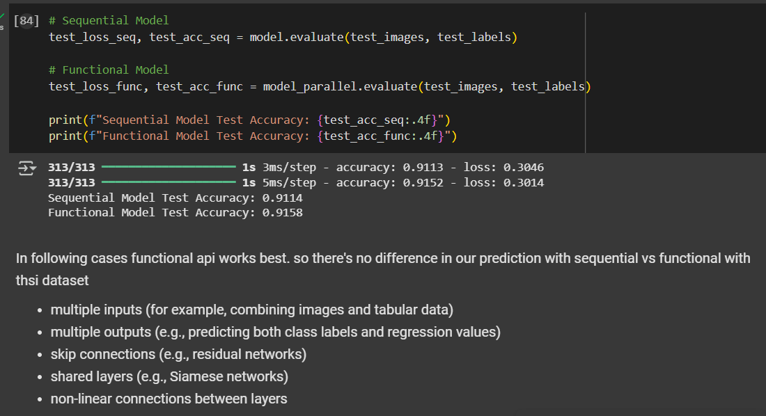
I rebuilt the same model using the Functional API to see the syntax shift:
-
Input Layer: Explicitly defined with
Input(shape=(28,28,1)). -
Layer Connections: Layers are chained like functions:
x = Conv2D(32, (3,3)(input_layer) x = MaxPooling2D()(x) ... -
Model Definition: Declared inputs/outputs explicitly:
model_func = Model(inputs=input_layer, outputs=output
Truncated — view the full README on GitHub.
Similar repos


Languages
Jupyter Notebook
99.8%
A year long journey with ai from data, exploring adjacent techs
Jupyter Notebook
50
960 commits
updated Dec 26, 2025
README
[!note]
I'll share progress and demos on linkedin and twitter.
I won’t post daily or raw learns, updates will be for specific topics, concise, and focused on what i actually built or explored. plan is 4–5 posts per week.
This journey is about AI from scratch with data, not my entire learning history. I’ll keep building in public while also learning other adjacent techs beyond AI.
Projects Completed
| Projects | Description | Deployment |
|---|---|---|
| Football Players Market Value Prediction | A 10-day end-to-end machine learning capstone project involving data scraping, cleaning, feature engineering, model training, and deployment. Achieved 94% accuracy using gradient boosting algorithms. | Live Demo 👆🏽 |
| Movie Recommender System | An end-to-end content-based movie recommender system leveraging a dataset of 5000 movies from Kaggle. Built with cosine similarity and TF-IDF vectorization. | Live Demo 👆🏽 |
| Cat vs Dog Classifier | A deep learning model leveraging VGG16 architecture, trained on an RTX 3050 Ti for 30 epochs, achieving 95% accuracy using the Kaggle Dogs vs Cats dataset. | Live Demo 👆🏽 |
| Guess The Footballer By Eyes | An interactive game where users compete against AI to recognize 25 famous footballers by their eyes alone. Built with ResNet18 achieving ~70% accuracy. Features scoring system and streak tracking. | Demo 👆🏽 |
| Seq2Seq Chatbot | A sequence-to-sequence chatbot trained on Cornell Movie-Dialogs Corpus using encoder-decoder architecture with Luong attention mechanism. Built from scratch in PyTorch. | Live Demo 👆🏽 |
| GPT from Scratch | Complete implementation of GPT transformer architecture from scratch following Karpathy's tutorial. Includes bigram model, self-attention, multi-head attention, and complete transformer blocks. | Notebook 📓 |
| Image Captioning | An end-to-end image captioning project using the Flickr8k dataset. Explored the "Show, Attend & Tell" paper, built vocabulary, extracted features with ResNet-18, and trained a transformer decoder. Achieved a BLEU-4 score of 0.18 and deployed a Streamlit demo app. | Live Demo 👆🏽 |
| cineRank - A movie ranker app | Community-driven movie leaderboard app with trending picks, sentiment reviews, and personal watchlists. Built using IMDb reviews, advanced text cleaning, EDA, vectorization (BoW, TF-IDF, GloVe, BERT), and BERT fine-tuning for sentiment classification. Features leaderboard, watchlists, and real-time updates. | Live Demo 👆🏽 |
| Choose Your Own Adventure | Inspired by interactive fiction like AI Dungeon, this app lets you become the protagonist in a personalized adventure story. Enter any theme—haunted mansions, space exploration, and more—and AI generates a unique branching narrative with multiple paths and endings. Features include an interactive visual map, concise story nodes (~40 words), meaningful choices, and a clean black-and-white interface for all devices. Explore different decision paths and control your own dynamic storytelling experience. | Project Demo 👆🏽 |
| Projects-Based-GenAI | Hands-on GenAI projects including text generation, multimodal models, and advanced LLM fine-tuning. Explore practical implementations of state-of-the-art generative AI techniques. | Project folder |
| Project-Based-AgenticAI | Applied agentic AI projects focusing on autonomous agents, multi-agent systems, and real-world agentic workflows using LangGraph and LangChain. | Project folder |
Resources
Progress
| Days | Date | Topics | Resources |
|---|---|---|---|
| Day1 | 2024‑12‑14 | Basics of Linear Algebra | 3blue1brown |
| Day2 | 2024-12-15 | Decomposition, Derivation, Integration, and Gradient Descent | 3blue1brown |
| Day3 | 2024-12-16 | Supervised Learning, Regression and classification | Machine Learning Specialization |
| Day4 | 2024-12-17 | Unsupervised Learning: Clustering and dimensionality reduction | Machine Learning Specialization |
| Day5 | 2024-12-18 | Univariate linear Regression | Machine Learning Specialization |
| Day6 | 2024-12-19 | Cost Functions | Machine Learning Specialization |
| Day7 | 2024-12-20 | Gradient Descent | CampusX, Machine Learning Specialization |
| Day8 | 2024-12-21 | Effect of learning Rate, Cost function and Data on GD | CampusX, Machine Learning Specialization |
| Day9 | 2024-12-22 | Linear Regression with multiple features, Vectorization | Machine Learning Specialization |
| Day10 | 2024-12-23 | Feature Scaling, Visualization of Multiple Regression and Polynomial Regression | Machine Learning Specialization |
| Day11 | 2024-12-24 | Feature Engineering, Polynomial Regression | Machine Learning Specialization |
| Day12 | 2024-12-25 | Scikit-Learn revision, Linear Regression using Scikit Learn | Machine Learning Specialization |
| Day13 | 2024-12-26 | LR lab, Classification | Machine Learning Specialization |
| Day14 | 2024-12-27 | Logistic Regression, Sigmoid Function | Machine Learning Specialization , CampusX |
| Day15 | 2024-12-28 | Decision Boundary, Cost Function | Machine Learning Specialization , CampusX |
| Day16 | 2024-12-29 | Gradient Descent for logical regression | Machine Learning Specialization , CampusX |
| Day17 | 2024-12-30 | Underfitting, Overfitting, Regularization Polynomial Features, Hyperparameters | Machine Learning Specialization |
| Day18 | 2024-12-31 | Neurons, Neural Netowrk, Forward Propagation | Machine Learning Specialization |
| Day19 | 2025-01-01 | Forward Propagation, Tensorflow implementations | Machine Learning Specialization |
| Day20 | 2025-01-02 | Building and comparing models (Binary Classification) | Machine Learning Specialization |
| Day21 | 2025-01-03 | Vectorization, Model training using Tensoflow | Machine Learning Specialization |
| Day22 | 2025-01-04 | Activation Functions, Softmax Intution | Machine Learning Specialization |
| Day23 | 2025-01-05 | Implementing Softmax | Machine Learning Specialization |
| Day24 | 2025-01-06 | Backpropagaton, What and how?? | Machine Learning Specialization |
| Day25 | 2025-01-07 | Backpropagation - Why? Advices for applying machine Learning | Machine Learning Specialization |
| Day26 | 2025-01-08 | Model selection, training test, cross validation, Bias and Variance, Learning curves | Machine Learning Specialization |
| Day27 | 2025-01-09 | Machine Learning Development Process, ML workflow | Machine Learning Specialization |
| Day28 | 2025-01-10 | Implementing ML model: Error Analysis and Transfer Learning | Notebook: Implementation, Machine Learning Specialization |
| Day29 | 2025-01-11 | Error Metrices, Encoding of Categorical Data, Transoformers | Machine Learning Specialization , CampusX |
| Day30 | 2025-01-12 | Scikit-Learn Pipelines & Ridge Regression (L2 Regularization) | Documentation: Scikit-Learn , CampusX |
| Day31 | 2025-01-13 | Lasso Regression (L1 Regularization), Elastic Net Regularization | ML playlist @CampusX |
| Day32 | 2025-01-14 | Decision Tree Emtropy and Information Gain | ML playlist @CampusX |
| Day33 | 2025-01-15 | Hyperparameters of Decision Tree with Scikit Learn, Regression Trees | ML playlist @CampusX , Visualize Yourself>> |
| Day34 | 2025-01-16 | Visualization Using DtreeViz(), Ensemble Learning | Github Repo: Dtreeviz, ML playlist @CampusX |
| Day35 | 2025-01-17 | Voting Ensemble >> Classification and Regression | ML playlist @CampusX , Visualize Yourself |
| Day36 | 2025-01-18 | Bagging Ensemble > Classification and Regression | ML playlist @CampusX |
| Day37 | 2025-01-19 | Random Forest: Intution, Working and difference with bagging, Random Forest Hyperparameters | ML playlist @CampusX |
| Day38 | 2025-01-20 | Boosting Ensemble: Adaboost Boosting | ML playlist @CampusX |
| Day39 | 2025-01-21 | Understanding GradientBoosting with Regression | ML playlist @CampusX |
| Day40 | 2025-01-22 | Gradient Boosting with Classification | ML playlist @CampusX , Vlog Link |
| Day41 | 2025-01-23 | XGboost Introduction | ML playlist @CampusX |
| Day42 | 2025-01-24 | XGBoost for Regression and Classification, Catboost Vs XGboost Vs LightGBM | ML playlist @CampusX ,Research Paper |
| Day43 | 2025-01-25 | Stacking Ensemble, Understanding Blending and K fold | ML playlist @CampusX |
| Day44 | 2025-01-26 | K-Nearest Neighbor, Coding KNN from Scratch | ML playlist @CampusX |
| Day45 | 2025-01-27 | Support Vector Machine | ML playlist @CampusX |
| Day46 | 2025-01-28 | K-Means Clustering, DBSCAN | Notebook: K-Means clustering Demo , Notebook: DBSCAN demo |
| Day47 | 2025-01-29 | Hierarchical Clustering, Silhouette Score | Kaggle, ML playlist @CampusX |
| Day49 | 2025-01-30 | PCA (Principle Component Analysis), Implementing with MNIST dataset | Notebook: Applying PCA on MNIST dataset |
| Day50 | 2025-02-01 | Visualizing and Comparing PCA, t-SNE, UMAP, and LDA + Revision with the course ML specialization | Machine Learning Specialization |
| Day51 | 2025-02-02 | Anomaly Detection | Machine Learning Specialization, Notebook: Anomaly Detection |
| Day52 | 2025-02-03 | Collaborative Filtering | Machine Learning Specialization |
| Day53 | 2025-02-04 | Project @ Football Players Market Value Prediction - Introduction and Planning | Project Plan |
| Day54 | 2025-02-05 | Project @ Football Players Market Value Prediction - Collecting Data (Scraping) | Notebook |
| Day55 | 2025-02-06 | Project @ Football Players Market Value Prediction - Cleaning Data | Notebook |
| Day56 | 2025-02-07 | Project @ Football Players Market Value Prediction - EDA | Notebook |
| Day57 | 2025-02-08 | Project @ Football Players Market Value Prediction - Feature Engineering: (Creating features, Transforming Features) | Notebook |
| Day58 | 2025-02-09 | Project @ Football Players Market Value Prediction - ML: (Linear Regression with Refined Features and deploying with Streamlit) | Notebook |
| Day59 | 2025-02-10 | Project @ Complete Streamlit setup for Linear Regression | Streamlit Documentation |
| Day60 | 2025-02-11 | Project @ Testing Ridge, Lasso, and Decision Trees | Project @ Football Players Market Value Prediction |
| Day61 | 2025-02-12 | Project @ Had to hit reset from Feature Engineering | Project @ Football Players Market Value Prediction |
| Day62 | 2025-02-13 | Project @ Finalizing Project and Deploying it | Project @ Football Players Market Value Prediction |
| Day63 | 2025-02-14 | Content-Based Movie Recommender System - Preprocessing | Notebook |
| Day64 | 2025-02-15 | Content-Based Movie Recommender System - Building and Deployment | Live Demo |
| Day65 | 2025-02-16 | Diving into Deep Learning | Intro to Deep Learning @MIT |
| Day66 | 2025-02-17 | Perceptrons | Deep learning playlist @ CampusX |
| Day67 | 2025-02-18 | Perceptron, Loss function and gradient Descent | Deep learning playlist @ CampusX , Grokking Deep Learning @Andrew W. Trask |
| Day68 | 2025-02-19 | Multilayer Perceptron | Deep learning playlist @ CampusX |
| Day69 | 2025-02-20 | MLP notation, Forward Propagation | Deep learning playlist @ CampusX |
| Day70 | 2025-02-21 | Loss Functions for deep learning | Deep learning playlist @ CampusX |
| Day71 | 2025-02-22 | Backpropagation, deep diving this time | Deep learning playlist @ CampusX |
| Day72 | 2025-02-23 | Implementing Backpropagation for Regression | Notebook: Backpropagation Regression |
| Day73 | 2025-02-24 | Implementing Backpropagation for Classification | Notebook: Implementation Backprop Classification |
| Day74 | 2025-02-25 | Revising old days, Memoization | Deep learning playlist @ CampusX |
| Day75 | 2025-02-26 | Vanishing Gradient, Exploding Gradient | Deep learning playlist @ CampusX |
| Day76 | 2025-02-27 | Implementing artificial neural networks (ann) for different datasets | Deep learning playlist @ CampusX |
| Day77 | 2025-02-28 | Improving Neural Networks | Deep learning playlist @ CampusX |
| Day78 | 2025-03-01 | Sequence Modeling / RNNs - Just Overview | Intro to Deep Learning @MIT |
| Day79 | 2025-03-02 | Transformers Attention - Just Overview | Intro to Deep Learning @MIT |
| Day80 | 2025-03-03 | CNNs - Just Overview Part 1 | Intro to Deep Learning @MIT |
| Day81 | 2025-03-04 | CNNs - Just Overview Part 2 | Intro to Deep Learning @MIT |
| Day82 | 2025-03-05 | Deep Generative Modeling - Just Overview | Intro to Deep Learning @MIT |
| Day83 | 2025-03-06 | Reinforcement Learning - Just Overview | Intro to Deep Learning @MIT |
| Day84 | 2025-03-07 | Deep Learning: Challenges & New Frontiers - Just Overview | Intro to Deep Learning @MIT |
| Day85 | 2025-03-08 | Early Stopping & Normalizing Inputs, Droput | Deep learning playlist @ CampusX, Grokking Deep Learning @Andrew W. Trask |
| Day86 | 2025-03-09 | Regularization, Quantization | Deep learning playlist @ CampusX |
| Day87 | 2025-03-10 | Activation Functions - Revisited | Deep learning playlist @ CampusX |
| Day88 | 2025-03-11 | Weight Initialization | Deep learning playlist @ CampusX |
| Day89 | 2025-03-12 | Deep Learning Optimizers | Deep learning playlist @ CampusX |
| Day90 | 2025-03-13 | Keras Tuner | Deep learning playlist @ CampusX |
| Day91 | 2025-03-14 | Deep Diving into CNNs | Deep learning playlist @ CampusX |
| Day92 | 2025-03-15 | Understanding Paddings and Strides | Deep learning playlist @ CampusX |
| Day93 | 2025-03-16 | Backpropagation in CNNs: A Quick Breakdown | Deep learning playlist @ CampusX, Grokking Deep Learning @Andrew W. Trask |
| Day94 | 2025-03-17 | LeNet5, Cat Vs Dog Classification | Deep learning playlist @ CampusX, Grokking Deep Learning @Andrew W. Trask |
| Day95 | 2025-03-18 | GPU slow than CPU - well in my case? | Deep learning playlist @ CampusX |
| Day96 | 2025-03-19 | Data Augmentation, Pretrained Models | Deep learning playlist @ CampusX, Grokking Deep Learning @Andrew W. Trask |
| Day97 | 2025-03-20 | Visualizing Convolutional Layers, Transfer Learning | Deep learning playlist @ CampusX, Grokking Deep Learning @Andrew W. Trask |
| Day98 | 2025-03-21 | Keras Functional API | Deep learning playlist @ CampusX , Article |
| Day99 | 2025-03-21 | Finalizing Dog Cat Classifier Project | Project - Live Demo |
| Day100 | 2025-03-23 | Hidden Markov Model, Quantum Machine Learning | Medium Article: Understanding Hidden Markov Models |
| Day101 | 2025-03-24 | Exploring Pytorch Surfacely | DL with Pytorch - Datacamp |
| Day102 | 2025-03-25 | Training a neural network with pytorch | DL with Pytorch - Datacamp |
| Day103 | 2025-03-26 | Evaluating and improving models | DL with Pytorch - Datacamp |
| Day104 | 2025-03-27 | Crawling through DL with pytroch | Deep Learning for Coders -Fast.Ai, @CampusX |
| Day105 | 2025-03-28 | Starting chapter 2 : from model to production | Deep Learning for Coders -Fast.Ai, @CampusX |
| Day106 | 2025-03-29 | Exploring Autograd and Portfolio Tweaks | Deep Learning for Coders -Fast.Ai, @CampusX |
| Day107 | 2025-03-30 | Refining Portfolio whole day | Deep Learning for Coders -Fast.Ai, @CampusX |
| Day108 | 2025-03-31 | Autograd in PyTorch: Deeper Understanding | Deep Learning for Coders -Fast.Ai, @CampusX |
| Day109 | 2025-04-01 | PyTorch Training Pipeline (Manual + Using nn.Module) | Deep Learning for Coders -Fast.Ai, @CampusX |
| Day110 | 2025-04-02 | Dataset & DataLoader Class in PyTorch | Deep Learning for Coders -Fast.Ai, @CampusX |
| Day111 | 2025-04-03 | ANN on Fashion MNIST, GELU | Deep Learning for Coders -Fast.Ai, @CampusX |
| Day112 | 2025-04-04 | ANN on larger FMNIST dataset with GPU (local), GELU/SiLU history | Deep Learning for Coders -Fast.Ai, @CampusX |
| Day113 | 2025-04-05 | Optimizing FMNIST NN using Dropouts, Regularization and Batch Normalization in Pytorch | Notebook |
| Day114 | 2025-04-08 | RNNs revisited, Karpathy's blog, Project Planning | Karpathy Blog |
| Day115 | 2025-07-08 | Classifying Footballers with their Eyes - Day 1 | Project Notebook |
| Day116 | 2025-07-09 | Classifying Footballers with their Eyes – Day 2 | Project Notebook |
| Day117 | 2025-07-10 | YOLO (You Only Look Once) | YOLO Paper |
| Day118 | 2025-07-11 | LSTM, GRU & Encoder-Decoder Architecture | Colah's Blog |
| Day119 | 2025-07-12 | Bahdanau Attention and Luong Attention | Bahdanau Paper |
| Day120 | 2025-07-13 | Building a Seq2Seq Chatbot – Data Preparation & Preprocessing | PyTorch Tutorial |
| Day121 | 2025-07-14 | Building a Seq2Seq Chatbot - Defining Model (encoder, attention, decoder) | Notebook |
| Day122 | 2025-07-15 | Building a Seq2Seq Chatbot – Evaluation / Deployment | Live Demo |
| Day123 | 2025-07-20 | Transformers – Deep Dive into Attention and Architecture | Attention Paper |
| Day124 | 2025-07-21 | Transformers – Vitals [understanding everything] | Transformer Guide |
| Day125 | 2025-07-22 | GPT from Scratch - Project Setup | Karpathy's Tutorial |
| Day126 | 2025-07-23 | GPT from Scratch - Bigram Language Model | Notebook |
| Day127 | 2025-07-24 | GPT from Scratch - Self-Attention | Notebook |
| Day128 | 2025-07-25 | GPT from Scratch – Complete Transformer | Notebook |
| Day129 | 2025-07-26 | Image Captioning – Kickoff | Notebook |
| Day130 | 2025-07-27 | Image Captioning – Feature Extraction & Pipeline | Notebook |
| Day131 | 2025‑07‑28 | Image Captioning – Training & Deployment | Build a Large Language Model from Scratch |
| Day132 | 2025‑07‑29 | Tokenizer Tricks (Subword, Byte-Pair Encoding) + Comparing Architectures | Build a Large Language Model from Scratch |
| Day133 | 2025‑07‑30 | Implementing seq2seq (Diff Approach of Visualizations) | Build a Large Language Model from Scratch |
| Day134 | 2025‑07‑31 | Implementing Transformer Encoder/Decoder Again | Build a Large Language Model from Scratch |
| Day135 | 2025‑08‑01 | Pretraining on Unlabeled Data, Evaluating, Loading Pretrained Weights | Build a Large Language Model from Scratch |
| Day136 | 2025‑08‑02 | Finetuning – Classification | Build a Large Language Model from Scratch |
| Day137 | 2025‑08‑03 | Finetuning – Teaching LLMs to Follow Prompts and Perform Complex Tasks, Visualizations | Build a Large Language Model from Scratch |
| Day137 | 2025‑08‑03 | Finetuning – Teaching LLMs to Follow Prompts and Perform Complex Tasks, Visualizations | Build a Large Language Model from Scratch |
| Day138 | 2025‑08‑04 | LLM Fine-Tuning & Evaluation | Build a Large Language Model from Scratch |
| Day139 | 2025‑08‑05 | Exploring Hugging Face Transformers | Build a Large Language Model from Scratch |
| Day140 | 2025‑08‑06 | Project – Sentiment Analysis [Planning] + Exploring ViT | Notebook, Kaggle Code |
| Day141 | 2025‑08‑07 | Project – Sentiment Analysis [Preprocessing] + ViT Architecture | Kaggle Code |
| Day142 | 2025‑08‑08 | Project – Sentiment Analysis [EDA + Testing GloVe] | Notebook, Notebook, Kaggle Code |
| Day143 | 2025‑08‑09 | Project – Sentiment Analysis [Advanced Architectures] | Notebook, Notebook, Kaggle Code |
| Day144 | 2025‑08‑10 | Project – Sentiment Analysis [App Deployment] | Live Demo, Code |
| Day145 | 2025‑08‑11 | Diving Deep into Vision Transformers (ViTs) | Blog |
| Day146 | 2025‑08‑12 | Diving into Diffusion Models | Video |
| Day147 | 2025‑08‑13 | Diffusion Model Deep Dive | Paper |
| Day148 | 2025‑08‑15 | Naive Bayes & Gaussian Mixture Models | Langchain Playlist |
| Day149 | 2025‑08‑17 | Introduction to Langchain | Langchain Playlist |
| Day150 | 2025‑08‑18 | Introduction to Langchain Components | Langchain Playlist |
| Day151 | 2025‑08‑19 | Deep Dive into Langchain Models | Langchain Playlist |
| Day152 | 2025‑08‑20 | Langchain Prompts and Building a Simple Chatbot | Langchain Playlist |
| Day153 | 2025‑08‑21 | Structured Output with Langchain | Langchain Playlist |
| Day154 | 2025‑08‑23 | Langchain Output Parsers | Langchain Playlist |
| Day155 | 2025‑08‑24 | Langchain Chain Fundamentals (Simple, Sequential, Parallel, Conditional Chains) | Langchain Playlist |
| Day156 | 2025‑08‑25 | Langchain Runnables (Modular Components, Composable Workflows) | Langchain Playlist |
| Day157 | 2025‑08‑26 | Runnable Modules Deep Dive (Sequence, Parallel, Passthrough, Lambda, Branch) | Langchain Playlist |
| Day158 | 2025‑08‑27 | Document Loaders & Text Splitters (RAG Foundations) | Langchain Playlist |
| Day159 | 2025‑08‑28 | Vector Stores in Langchain (Chroma, CRUD Operations, Similarity Search) | Langchain Playlist |
| Day160 | 2025‑08‑29 | Retrievers & Few-Shot Learning (Wikipedia, Vector, MMR, MultiQuery, Contextual) | Langchain Playlist |
| Day161 | 2025‑08‑30 | RAG Application for UCL Draw (Text Splitting, Vector Embeddings, Response Generation) | Langchain Playlist |
| Day162 | 2025‑08‑31 | Langchain Tools (Built-in & Custom, Tool Calling & Binding) | Langchain Playlist |
| Day163 | 2025‑09‑01 | Langchain Agents (Zero-Shot, Conversational, ReAct DocStore, Self-Ask) | Langchain Playlist |
| Day164 | 2025‑09‑02 | Local Agent with Ollama & Langchain (ChromaDB, RAG) | Langchain Playlist |
| Day165 | 2025‑09‑03 | Introduction to LangGraph (Stateful Agent Workflows) | Langgraph Playlist |
| Day166 | 2025‑09‑04 | Agentic AI Fundamentals (Autonomy, Components, Planning, Memory) | Langchain Playlist |
| Day167 | 2025‑09‑05 | LangChain vs LangGraph Comparison (State Management, Chatbot Example) | Langgraph Playlist |
| Day168 | 2025-09-06 | Building a Branching Chatbot | Langgraph Playlist |
| Day169 | 2025-09-07 | Persistence with Checkpoints | Langgraph Playlist |
| Day170 | 2025-09-08 | Exploring LangSmith | Langgraph Playlist |
| Day171 | 2025-09-11 | Contextual Q&A with Memory | Langchain Playlist |
| Day172 | 2025-09-12 | Bhagavad Gita Expert Chatbot | Langgraph Playlist |
| Day173 | 2025-09-13 | Multi-Agent Debating System | Langgraph Playlist |
| Day174 | 2025-09-14 | Debate Agent App Completion | Langgraph Playlist |
| Day175 | 2025-09-15 | Introduction to FastAPI for ML | FastAPI Documentation |
| Day176 | 2025-09-16 | FastAPI Implementation | FastAPI Documentation |
| Day177 | 2025-09-17 | HTTP Request Methods and REST Architecture | FastAPI Documentation |
| Day178 | 2025-09-18 | FastAPI Parameters and Request Body | FastAPI Documentation |
| Day179 | 2025-09-19 | Mini Project with FastAPI | FastAPI Documentation |
| Day180 | 2025-09-20 | Building Industry-Ready APIs with FastAPI | FastAPI Documentation |
| Day181 | 2025-09-23 | Containerizing FastAPI Applications | FastAPI Documentation |
| Day182 | 2025-09-24 | fastapi deployment on aws | aws docs |
| Day183 | 2025-09-25 | project setup – choose your own adventure | project repo |
| Day184 | 2025-09-26 | database design and core components | project repo |
| Day185 | 2025-09-27 | api implementation and background tasks | project repo |
| Day186 | 2025-09-28 | backend completion and debugging | project repo |
| Day187 | 2025-09-29 | frontend integration and project completion | project repo |
| Day188 | 2025-10-01 | concurrency patterns in fastapi | starlette concurrency |
| Day189 | 2025‑10‑02 | self-supervised learning – foundations | Lil'Log SSL Blog |
| Day190 | 2025‑10‑03 | mcp and lazy week | Masked Conditional Prediction |
| Day191 | 2025‑10‑04 | ssrl – image & video approaches | Lil'Log SSRL |
| Day192 | 2025‑10‑05 | wrapping up ssl + fun reads | Postgres vs SQLite, GPT Speculations |
| Day193 | 2025‑10‑06 | llama2 fine-tuning with qlora | QLoRA Fine-Tuning Guide |
| Day194 | 2025‑10‑12 | gemma 2 fine-tuning using unsloth | Gemma2 Fine-tuning Notebook |
| Day195 | 2025‑10‑13 | saving & loading lora adapters, explored "lora without regret" | LoRA Blog Post |
| Day196 | 2025‑10‑14 | attempted RAG evaluation, faced compatibility issues | MCP Documentation |
| Day197 | 2025‑10‑16 | built a custom MCP server, integrated with Cursor | Custom Implementation |
| Day198 | 2025‑10‑18 | studied RL fundamentals: policies, MDPs, rewards | HuggingFace RL Course |
| Day199 | 2025‑10‑20 | explored Q-learning & Deep Q-learning, lunar lander env | HuggingFace RL Course |
| Day200 | 2025‑10‑21 | trained PPO agent on LunarLander-v3 using SB3 | HuggingFace RL Course |
Day 01: Basics of Linear Algebra
linear algebra is used to represent data, perform matrix operations, and solve equations in algorithms like regression, pca, and neural networks.
-
Scalars, Vectors, Matrices, Tensors: Basic data structures for ML.
-
Linear Combination and Span: Representing data points as weighted sums. Used in Linear Regression and neural networks.
-
Determinants: Matrix invertibility, unique solutions in linear regression.
-
Dot and Cross Product: Similarity (e.g., in SVMs) and vector transformations.
Slow progress right?? but consistent wins the race!
Day 02: Decomposition, Derivation, Integration, and Gradient Descent
-
Identity and Inverse Matrices: Solving equations (e.g., linear regression) and optimization (e.g., gradient descent).
-
Eigenvalues and Eigenvectors: PCA, SVD, feature extraction; eigenvalues capture variance.
-
Singular Value Decomposition (SVD): PCA, image compression, and collaborative filtering.
Calculus Overview:
-
Functions & Graphs: Relationship between input (e.g., house size) and output (e.g., house price).
-
Derivatives: Adjust model parameters to minimize error in predictions (e.g., house price).
-
Partial Derivatives: Measure change with respect to one variable, used in neural networks for weight updates.
-
Gradient Descent: Optimization to minimize the cost function (error).
-
Optimization: Finding the best values (minima/maxima) of a function to improve predictions.
-
Integrals: Calculate area under a curve, used in probabilistic models (e.g., Naive Bayes).
Revised statistics and probability concepts. Ready for the ML Specialization course!
Day 03: Supervised Machine Learning: Regression and Classificaiton
- Supervised Learning:
- Regression:
- Classification:
Day 04: Unsupervised Learning: Clustering, dimensionality reduction
data only comes with input x, but not output labels y. Algorithm has to find structure in data.
- Clustering: group similar data points together
- dimensionality reduction: compress data using fewer numbers eg image compression
- anomaly detection: find unusual data points eg fraud detection
Day 05: Univariate Linear Regression:
- Learned univariate linear regression and practiced building a model to predict house prices using size as input, including defining the hypothesis function, making predictions, and visualizing results.
Notebook: Model Representation
- Univariate Linear Regression Quiz
Day 06: Cost Function:
Visualization of cost function:
- manually reading these contour plot is not effective or correct, as the complexity increases, we need an algorithm which figures out the values w, b (parameters) to get the best fit time, minimizing cost function
Notebook: Model Representation
Gradient descent is an algorithm which does this task
Day 07: Gradient Descent
learned the basics by assuming slope constant and with only the vertical shift.
later learned GD with both the parameters w and b.
Day 08: Effect of learning Rate, Cost function and Data on GD
- learning rate on GD:Affects the step size; too high can overshoot, too low can slow convergence
- cost function on GD:Smooth, convex functions help faster convergence; complex ones may trap in local minima
- Data on GD:Quality and scaling affect stability; more data improves gradient estimates
Notebook: gradient descent animation 3d
Day 09: Linear Regression with multiple features, Vectorization
Predicts target using multiple features, minimizing error.
- Vectorization: Matrix operations replace loops for faster calculations.
Day10: Feature Scaling
Today, I learned about feature scaling and how it helps improve predictions. There are multiple methods for feature scaling, including
- Min-Max Scaling
- Mean Normalization
- Z-Score Normalization
To ensure proper convergence:
check the learning curve to confirm the loss is decreasing.
Start with a small learning rate and gradually increase to find the optimal value.
Day 11: Feature engineering and Polynomial Regression
feature engineering improves features to better predict the target.
eg If we need to predict the cost of flooring and have length and breadth of the room as features, we can use feature engineering to create a new feature, area (length × breadth), which directly impacts the flooring cost.

explored polynomial regression that models the relationship between variables as a polynomial curve instead of a straight line
Equation:
y = b₀ + b₁x + b₂x² + ... + bₙxⁿ
It is useful for capturing nonlinear relationships in data.
Lab1: Feature Scaling and Learning Rate
Lab2: Feature Engineering and PolyRegression
Day 12: Linear Regression using Scikit Learn
Had a productive session with linear regression in scikit learn. The lab helped me get a better grasp of the process, though I need more practice with tuning models. Also revisited the Scikit-Learn models ,more comfortable with them now
- Scikit-learn is an open-source Python library used for machine learning that provides simple and efficient tools for data analysis, including algorithms for classification, regression, clustering, and dimensionality reduction.
Day 13: Classification
Notebook: Graded Lab
Notebook: Classification solution
- Classification is the process of categorizing items into different groups based on shared characteristics, like classifying tumors into benign (non-cancerous) and malignant (cancerous) based on their growth behavior and potential to spread.
The example above demonstrates that the linear model is insufficient to model categorical data. The model can be extended as described in the following lab.
Day 14: Logistic Regression, Sigmoid Function
- Logistic Regression: A classification algorithm used to predict probabilities of binary outcomes.
- Sigmoid Function: A mathematical function that maps any input to a value between 0 and 1, used in logistic regression to model probabilities.
Day 15: Decision Boundary, Cost Function
- Decision Boundary: A line or surface that separates different classes in a classification problem based on the model’s predictions.
- cost function:
Day 16: Gradient Descent for Logical Regression
Notebook: Gradient Descent Model implementation
Notebook: GD with Scikit-learn
Learned logistic regression cost, gradient descent, and sigmoid derivatives through step-by-step derivations and comparisons with linear regression.
Day 17: Underfitting, Overfitting
Today, explored teh concepts, overfitting (high variance), underfitting (high bias) and generalization(just right). Regularization to reduce Overfitting. Explored Regularized logistic regression.
- If the data is in non linear behaviour then we have to appply Ml algos like decision tree, random forest and svm.
Explored hypermeters of logistic regression, and gained some knowledge.
Day 18: Neurons, Layer, Neural netowrk, forward propagation
-
neural network: neural networks are machine learning algorithms that model complex patterns using multiple hidden layers and non-linear activation functions. they take inputs, pass them through hidden layers of neurons, and output a prediction.
-
Neurons: a neuron takes weighted inputs, applies an activation function, and outputs a result. inputs can be features or outputs from previous neurons, with weights adjusting their influence.
fig: single neuron in action -
Synapse: synapses connect neurons and carry the weighted inputs. each connection has a weight that adjusts during training.
-
weights: weights control the strength of connections between neurons. they are multiplied by inputs to influence the output, and are adjusted during training.
Popular activation functions include relu and sigmoid.
-
Bias: bias is a constant added to the weighted input before applying the activation function, helping the model represent patterns that don’t pass through the origin.
-
Layers:
- input layer: holds the data for the model, with each neuron representing an attribute.
- hidden layer: applies activation functions to the inputs and passes results to the next layer.
- output layer: receives input from the last hidden layer and returns the model’s prediction.
Day 19: Forward Propagation
- Forward Propagation: Input data is “forward propagated” through the network layer by layer to the final layer which outputs a prediction.
Notes for today:
Matrix Representation:
How forward Prop works for digit classification??
Notebook: Neurons and Layers
Notebook: A small Neural Netowrk using tensoflow
- tensorflow basics:
-
representation of data:numpy arrays used for input (e.g., 2D arrays).
x = np.array([[1, 2, 3], [4, 5, 6]]) -
building a neural network:
-
define layers:
layer1 = dense(units=25, activation='sigmoid') layer2 = dense(units=15, activation='sigmoid') layer3 = dense(units=1, activation='sigmoid') -
stack layers in a model:
model = sequential([layer1, layer2, layer3]) -
compile and train:
model.compile(optimizer='adam', loss='binary_crossentropy')
model.fit(x, y, epochs=10)
-
-
visualization:neurons connect layer by layer, with weights and biases computed at each step (refer to attached gif).
-
Day 20: Python Implementation from Scratch
Implemented forward propagation to compute predictions and backpropagation to optimize weights for binary classification.
- AGI: An advanced AI capable of generalizing across tasks like humans.
Day 21: Vectorization, Model Training
Exploredd Vectorization for efficient computation
- Tensorflow: model.compile, binary_crossentropy, model.fit trained a binary classification model and tested its accuracy
Training Model with tensorflow:
Notes for today:
Day 22: Activation Functions, Softmax
the universal approximation theorem explains that a neural network with enough hidden neurons and non-linear activations like sigmoid or relu can approximate almost any function, even complex patterns like wavy graphs.
Activation Functions:
commonly used activation functions include:
- sigmoid: squashes values between 0 and 1, often used for binary classification.
- relu: outputs 0 for negatives and the input itself for positives, commonly used in hidden layers.
- tanh: outputs between -1 and 1, useful for centered data.
for multiclass classification, softmax is ideal in the output layer as it converts logits into probabilities that sum to 1. during training, the model adjusts weights to maximize the correct class probability, using categorical cross-entropy loss. softmax generalizes logistic regression, which is typically used for binary classification. in both, activation and loss functions differ based on the output type.
Logistic Vs softmax:
Notes:
Day 23: Implementation of Softmax Regression
- Classification with multiple Outputs: PS: there's difference between multiclass classificaiton and multilabel classification Notebook: Softmax/Multinomial in Iris dataset- Multilabel
NOTE: softmax regression is a classification algorithm that calculates probabilities for multiple classes using a linear combination of inputs and the softmax function. the class with the highest probability is chosen as the prediction
Improved Implementation of Softmax:
Tensorflow implementation:
model = Sequential(
    [
        Dense(25, activation = 'relu'),
        Dense(15, activation = 'relu'),
        Dense(4, activation = 'softmax')    # < softmax activation here

        ##         Dense(4, activation = 'linear')   #<-- Note
    ]
)
model.compile(
    loss=tf.keras.losses.SparseCategoricalCrossentropy(),
    ##     loss=tf.keras.losses.SparseCategoricalCrossentropy(from_logits=True),  #<-- Note ---- This is preferred model softmax and loss are combined for more accurate result.
    optimizer=tf.keras.optimizers.Adam(0.001),
)

model.fit(
    X_train,y_train,
    epochs=10
)
Day 24: Backpropagation - what and how ?
- what? Backpropagation adjusts nneural network weights by propagating errors backward using the chain rule and optimizing them with gradient descent.
- how? Forward pass to compute outputs, Calculate errors, propagate them backward, and update weights iteratively. Take a look at document below.
Backpropagation example with Neural Network:
Notes:
Day 25: Backpropagation - Why? Advices for applying machine Learning
Today, I dived into the reasons behind backpropagation's effectiveness in training neural networks. It's not just about adjusting weights; it's the gradients that guide optimization, helping the model minimize error and improve predictions. The backpropagation process makes sure that the error gets distributed in a way that leads to better learning.
How????
- Gradients: they ensure efficient error minimization by guiding weight updates.
- Optimization: properly tuned gradients lead to smoother optimization and faster convergence.
- Model Evaluation: evaluating model performance becomes easier with backpropagation because of the systematic error propagation and weight adjustments.
Notes:
Day 26: Model selection and training/cross validation/test sets, Bias and Variance
mnist dataset: Label and our prediction after training
Errors in our prediction:
- the importance of splitting data into training, validation, and test sets cross-validation and its role in hyperparameter tuning.
- Diagnosing bias and variance with error trends: high bias = underfit, high variance = overfit.
- regulariaztion to handle the tradeoff between bias and variance.
- how learning curves reveal insights about model performance and whether gathering more data will help.
Notes:
Notebook: Practice Lab: Neural Networks for Handwritten Digit Recognition, Multiclass
Notebook: Diagnosing Bias and Variance
Notebook: Model Evaluation and selection
Day 27: Machine Learning Development Process, ML workflow
machine learning development process
- ml development is iterative, involving:
- choosing model and data architecture.
- training the model.
- diagnosing bias, variance, and errors.
2. error analysis: identify and fix patterns in model failures.
3. adding data:
- data augmentation: modify existing data (e.g., distortions).
- data synthesis: create artificial data.
-
transfer learning:
- reuse pre-trained models for similar tasks.
- fine-tune them with your own data.
-
ml projects follow these steps:
- data collection.
- preprocessing.
- modeling.
- evaluation.
- deployment.
- monitoring.
-
ethics and fairness -
ensure ethical use by:- avoiding biased decisions in loans, jobs, etc.
- preventing harmful applications like deepfakes.
Notes:
Day 28: Machine Learning Model: Error Analysis and Transfer Learning
Notebook: Code Implementation from Scratch
-
Confusion Matrix Analysis: the most frequent error is misclassifying 5 as 3. overall, the error rate is around 8%.
-
Iterations Insight: after 200 iterations, the error rate does not decrease significantly, suggesting that 200 iterations are enough for the model to converge.
-
Data Augmentation Insight: despite applying data augmentation, there was no improvement in accuracy. this is because the MNIST dataset is already preprocessed, with centered and normalized images, making the augmentation techniques less effective. in general, data augmentation works best when the dataset is smaller or images are not preprocessed.
-
Transfer Learning with MobileNetV2:
- Training set accuracy improved from 56.95% to 73.02%.
- Validation accuracy increased from 70.52% to 74.06%.
- Loss decreased consistently for both training and validation sets, signaling better learning and generalization.
- The model shows significant improvement over epochs.
- Using transfer learning, the model started with an initial accuracy of 74% (pre-trained on ImageNet). As training progressed, the model continued to adapt, improving with each epoch. transfer learning was effective, yielding good results with fewer epochs.
Day 29: Error Metrices, Encoding of Categorical Data, Transoformers
Notebook: Lab week 3: Improving Model
Precision vs. Recall Trade-Off:
- High Precision: Only hire candidates you’re sure are good. Result: Fewer bad hires, but you might miss some great ones. Example: You hire 5 people, all are good, but you missed 10 other good ones.
- High Recall: Hire as many as possible to ensure no good candidate is missed. Result: You catch all great candidates but end up with some bad hires too. Example: You hire 50 people, 20 are good, but 30 are bad.
- When to Focus on Each?
-
Precision: When mistakes (bad hires) are costly. Example: Hiring a brain surgeon.
-
Recall: When missing good candidates is worse. Example: Hiring for a customer service team.
Encoding of Categoriical Data:
| Encoding Type | Use When | Example |
|---|---|---|
| Label Encoding | Small, unordered categories | Colors: [Red, Blue] |
| Ordinal Encoding | Ordered categories | Education: [Low, High] |
| One-Hot Encoding | Nominal data, fewer unique categories | Days: [Mon, Tue, Wed] |
Types of Transformers:
| Transformer | Purpose | Example Use Case | Input | Output |
|---|---|---|---|---|
| Column Transformer | Apply different transformations to different columns (e.g., scaling and encoding). | Scale age and one-hot encode city names. | Age: [25, 35, 45], City: [NY, LA, CHI] | [-1.22, 0, 0, 1], [0, 1, 0, 0], [1.22, 0, 1, 0] |
| Function Transformer | Apply a mathematical function (e.g., log or sqrt) to all values. | Apply logarithmic transformation to data. | [1, 10, 100] | [0.69, 2.39, 4.61] |
| Power Transformer | Normalize and reduce skewness in data, making it more Gaussian-like. | Stabilize variance in highly skewed data. | [1, 10, 100] | [-1.22, 0.0, 1.22] |
Day 30: Scikit-Learn Pipelines & Ridge Regression (L2 Regularization)
I explored how to create pipelines in Scikit-learn to streamline the process of combining multiple steps (like preprocessing, model fitting, and regularization) into a single object. This simplifies workflows and ensures reproducibility.
There are three techniques of regularization:
- Ridge (L2)
- Lasso (L1)
- Elastic Net (Combination)
Key Understanding of Ridge Regression:
- How the coefficient Get affected?
- Regularization shrinks the coefficients, preventing them from becoming too large, which reduces overfitting.
- Higher Values are impacted more
- The larger the regularization value (alpha), the more the coefficients are reduced.
- Impact on Bias Variance Tradeoff
- Higher regularization increases bias but reduces variance, making the model more generalizable.
- Effect on Loss Function
- adds a penalty term that limits the magnitude of the coefficients.
- Why Ridge Regression is called so?
- Named after the concept of creating a "ridge" or constraint on the model’s coefficients, preventing them from growing too large.
Notes:
Notebook: Key Understandings of ridge Regression
Day 31: Lasso Regression (L1 Regularization), Elastic Net Regularization
Lasso Regression:
-
How are coefficients affected by λ (alpha)? As λ increases, regularization strength grows, shrinking less important coefficients to exactly zero. Larger λ values lead to feature selection by removing irrelevant features.
-
Are higher coefficients affected more? No. Lasso affects smaller coefficients more, shrinking them to zero first. Larger coefficients remain relatively unaffected if they contribute significantly to the model.
-
Impact of λ on bias and variance:
- Higher λ increases bias (simpler model) and reduces variance.
- Lower λ reduces bias (complex model) but increases variance.
-
Effect of Regularization on Loss Function:
- Lasso add λ sum(w_i) to the loss, promoting sparsity by penalizing the absolute magnitude of coefficients. Unlike Ridge, it can remove features entirely, improving interpretability.
- Lasso add λ sum(w_i) to the loss, promoting sparsity by penalizing the absolute magnitude of coefficients. Unlike Ridge, it can remove features entirely, improving interpretability.
Elastic Net Regularization:
Elastic Net combines L1 (Lasso) and L2 (Ridge) penalties. It selects important features by shrinking some coefficients to zero (like Lasso) and handles correlated features by shrinking coefficients without setting them to zero (like Ridge). It’s useful when features are both highly correlated and some are irrelevant. Elastic Net is controlled by two parameters:
α (mix of Lasso and Ridge) and
λ (regularization strength).
Notes:
Day 32: Decision Tree: Entropy and Information Gain
A decision tree is a flowchart-like structure used for classification or regression, where data is split into branches based on conditions until a final decision (leaf) is reached.
- Decision Tree on Categorical Variables: Splits data based on categories like "Sunny" or "Rainy".
- Decision Tree on Numerical Variables: Splits data using thresholds like Age > 30.
- How Decision Tree Works: Repeatedly splits data into smaller groups based on conditions.
- Terminology: Root (start), Branch (path), Leaf (decision).
- Pro - Simple to understand; Con - Can overfit.
- Entropy: Measures uncertainty; low entropy = purer data.
- Entropy Calculation:
∑ p(x) * log2(p(x)). - Information Gain: Reduction in entropy after splitting data.
IG=Entropy(before)−Weighted Entropy(after) - Gini Impurity: Measures group purity, faster than entropy.
- Why Use Gini Over Entropy: Simpler and computationally faster.
Notes;
Day 33: Hyperparameters of DT with sclearn, Regression Trees:
Studied hyperparameters of Decision Trees in Scikit-learn and techniques to handle overfitting and underfitting.
- Criterion (gini, entropy, log loss): Determines the quality of a split.
- Splitter: Helps reduce overfitting with better random splits.
- Max Depth: Controls tree depth; too high causes overfitting, too low causes underfitting.
- Min Sample Split: Sets the minimum samples required to split a node.
- Min Sample Leaf: Sets the minimum samples per leaf.
- Max Features: Determines how many features to use for splits.
- Max Leaf Nodes: Limits the number of leaf nodes.
- Min Impurity Decrease: Controls splitting based on impurity reduction.
A Regression Tree predicts continuous variables by splitting data to minimize variance. The best split is determined by maximizing variance reduction, calculated as the variance of the root node minus the weighted average variance of the leaf nodes.
Code:
Output:
Day 34: Visualization Using dtreeviz, Ensemble Learning Overview
Notebook: Visualization of Decision Tree Official Notebook: Visualization of Decision Tree
- started learning about ensemble learning: understood the concept of "wisdom of the crowd" in ensemble methods. types of ensemble methods: voting, bagging, boosting, and stacking. overview of random forest and bootstrapped aggregation (bagging). learned how boosting adjusts predictions iteratively.
Visuals of Bagging, boosting and stacking:
Notes;
Day 35: Voting Ensemble > Classification and Regression
-
Soft voting: logistic regression: 60% fraud, random forest: 80% fraud, svm: 40% fraud → final probability: (60% + 80% + 40%) / 3 = 60%.
-
Hard voting: majority wins, logistic regression predicts "fraud," random forest predicts "not fraud," and svm predicts "fraud" → final prediction: "fraud."
Conclusions from Notebook: voting Classifier
-
weighted voting: assigning weights to classifiers helps emphasize stronger models, further improving performance.
-
same algorithm, different hyperparameters: tweaking hyperparameters (e.g., kernel degree in SVM) can lead to significant accuracy changes, highlighting the value of hyperparameter optimization.
Classification:
voting_clf = VotingClassifier(
    estimators=[
        ('lr', log_reg),  # logistic regression: good for linear patterns
        ('rf', rand_forest),  # random forest: captures complex relationships
        ('svc', svm_clf)  # support vector machine: handles edge cases
    ],
    voting='soft',  # averages probabilities from all models for final prediction
    weights=[2, 1, 1],  # gives higher importance to logistic regression
    n_jobs=-1  # enables parallel processing for faster training
)
What to use? soft voting or hard voting, depends if possible use both and then try to find out:
Regression:
- voting regressor combines multiple regression models to predict continuous values.
similarly, in regression, soft voting averages continuous predictions, and weighted voting helps models with higher performance contribute more.
Visualize voting regression here: link
voting_reg = VotingRegressor(
    estimators=[
        ('lr', lin_reg),  # linear regression: good for linear relationships
        ('rf', rand_forest_reg),  # random forest regressor: handles non-linear patterns
        ('svr', svr_clf)  # support vector regressor: captures complex relationships
    ],
    weights=[2, 1, 1],  # assigns higher importance to linear regression
    n_jobs=-1  # enables parallel processing for faster training
)
Day 36: Bagging Ensemble > Classification and Regression
-
bagging (bootstrap aggregating) is an ensemble learning technique that combines predictions from multiple models trained on different subsets of the data (created via bootstrapping) to improve accuracy and reduce variance.
-
Intution:
- random sampling: create multiple datasets by sampling with replacement from the original dataset.
- train independently: train a model (single preferred) on each bootstrapped dataset (e.g., decision trees).
- combine predictions: aggregate their predictions by majority voting (classification) or averaging (regression). this reduces overfitting and increases stability, especially for high-variance models.
Classification:
- Intution
- Code Demo
from sklearn.ensemble import BaggingClassifier
from sklearn.tree import DecisionTreeClassifier

# initialize the bagging classifier
bagging_model = BaggingClassifier(
    base_estimator=DecisionTreeClassifier(),  # base model for ensemble; here, decision trees
    n_estimators=10,                          # number of base models to train
    max_samples=1.0,                          # fraction of the dataset for each base model (1.0 = 100%)
    max_features=1.0,                         # fraction of features used in each bootstrap sample
    bootstrap=True,                           # sample datasets with replacement (True enables bootstrapping)
    bootstrap_features=False,                 # sample features with replacement (False = no feature bootstrapping)
    random_state=42                           # seed for reproducibility
)
Regression:
- Intution:
- Code Demo:
bagging_model = BaggingRegressor(
    base_estimator=DecisionTreeRegressor(),  # base model for ensemble; here, decision trees
    n_estimators=10,                          # number of base models to train
    max_samples=1.0,                          # fraction of the dataset for each base model (1.0 = 100%)
    max_features=1.0,                         # fraction of features used in each bootstrap sample
    bootstrap=True,                           # sample datasets with replacement (True enables bootstrapping)
    bootstrap_features=False,                 # sample features with replacement (False = no feature bootstrapping)
    random_state=42                           # seed for reproducibility
)
Day 37: Random Forest: Intution, Working and difference with bagging, Random Forest Hyperparameters
random forest is like a bunch of decision trees making a group decision. each tree gets a vote on the outcome, and the most votes win. it's like asking a bunch of experts for advice and going with the majority.
Sampling Techniques:
- row sampling
- column sampling
- combination
Random Forest vs bagging:
-
why random forest performs well: it reduces overfitting by averaging multiple decision trees trained on different random subsets of data and features, improving accuracy and robustness.
-
random forest vs bagging: both use multiple trees, but random forest adds feature randomness at each split, making trees less correlated and boosting performance.
Notebook: Random forest Vs bagging
Random forest Hyperparameters:
model = RandomForestClassifier(
    # core hyperparameters
    n_estimators=100,         # number of decision trees in the forest
    max_features="sqrt",      # max features to consider at each split
    max_depth=None,           # max depth of each tree; None = grow fully
    min_samples_split=2,      # min samples needed to split a node
    min_samples_leaf=1,       # min samples required in a leaf node
    bootstrap=True,           # with replacement or without replacement

    # advanced hyperparameters
    max_leaf_nodes=None,      # max number of leaf nodes per tree; None = unlimited
    min_weight_fraction_leaf=0.0,  # min fraction of total weight for a leaf node
    class_weight=None,        # weights for handling class imbalance (e.g., 'balanced')
    ccp_alpha=0.0,            # complexity parameter for pruning; trade-off between size and accuracy
    criterion="gini",         # metric to evaluate splits: "gini" (default) or "entropy"
    warm_start=False,         # reuse previous trees for incremental training; False = train from scratch
    oob_score=False,          # whether to use out-of-bag samples to estimate generalization accuracy
    verbose=0,                # verbosity of output (0 = silent)
    n_jobs=-1,                # number of CPU cores for parallel processing; -1 = use all cores
    random_state=42           # seed for reproducibility
)
Day 38: Boosting Ensemble: Adaboost Boosting
- boosting is a sequential ensemble learning method where models correct the errors of previous models to reduce bias.
combines weak learners (like decision stumps) to create a strong predictive model.
Notes:
AdaBoost Exploration:
step-by-step understanding of adaboost’s workflow, including:
- calculating sample weights and weak learner errors.
- updating model contributions based on performance.
- final prediction via weighted majority vote.
- visualized how adaboost focuses on difficult samples.
implemented adaboost from scratch without using sklearn.
Notebook: Adaboost Implementation
Day 39: Understanding GradientBoosting with Regression:
"a model that learns step-by-step by fixing the mistakes of the previous model."
- Comparision between Adaboost and Gradietn boost:
boosting + gradients (gradients = direction to minimize error).
pseudo-  residual = actual - predicted
new prediction = old prediction + (learning_rate × residual)
gradient boosting variations:
- xgboost: uses regularization and handles missing data efficiently.
- lightgbm: faster with large datasets.
- catboost: great for categorical data.
    gb = GradientBoostingRegressor(
        n_estimators=100,      # number of trees
        learning_rate=0.1,     # step size for updates
        max_depth=3,           # depth of each tree
        min_samples_split=2,   # min samples to split a node
        min_samples_leaf=1,    # min samples per leaf
        subsample=1.0,         # fraction of samples per tree
        max_features=None,     # use all features
        random_state=42        # ensures reproducibility
    )
Notes:
Day 40: Gradient Boosting with Classification
Overview
- Gradient boosting improves classification by minimizing log-loss iteratively.
- Each tree focuses on correcting errors made by previous trees.
- Uses gradients of the loss function to guide updates.
Algorithm
- Initialize predictions:
F0(x)(log-odds for classification). - For each iteration:
- Compute pseudo-residuals:
ri = - ∂(loss) / ∂F(xi) - Fit a weak learner (tree) to
ri. - Update predictions:
F(x) = F(x) + η * h(x)
whereηis the learning rate.
- Compute pseudo-residuals:
Loss Function
- Binary classification: log-loss.
Loss = -[y log(p) + (1 - y) log(1 - p)] - Multiclass classification: softmax loss.
gb = GradientBoostingClassifier(
    n_estimators=100,
    learning_rate=0.1,
    max_depth=3,
    random_state=42
)
Notes:
Notebook: Gradient Boosting Classification
Visuals:
Day 41: Variations of Gradient Boosting: XGBoost - Introduction.
- xgboost
- lightgbm
- catboost
XGBoost:
xgboost (eXtreme Gradient Boosting) is an advanced implementation of gradient boosting that addresses some key limitations in traditional gradient boosting and adaboost.
here's a quick rundown of what i've learned so far.
-
Flexibility
- cross-platform support means xgboost works on different operating systems without much hassle.
- it supports multiple languages like python, c++, and r, which makes it easy to integrate with your preferred tech stack.
- integrating with other libraries like scikit-learn or spark is a breeze.
- it can handle all kinds of ml problems — whether it's classification, regression, or ranking.
-
Speed
- parallel processing is key. it uses all your cores to speed things up, so you get faster results.
- optimized data structures (like DMatrix) help reduce memory usage and make computations more efficient.
- it’s cache-aware, so it knows how to make use of your cpu cache and speed up data retrieval.
- xgboost handles datasets larger than memory through out-of-core computing.
- distributed computing helps when your dataset is huge and you need to scale your work across multiple machines.
- with gpu support, xgboost accelerates matrix calculations, making it much faster for large datasets.
-
Performance (Why this is different from other algos??)
- regularization is a big win. it prevents overfitting with L1 and L2 regularization, keeping your model generalizable.
- it automatically handles missing values, learning the best way to fill them in.
- sparsity-aware split finding is great for sparse data (think text data or categorical features).
- finding efficient splits in trees is another xgboost feature that speeds up training without compromising accuracy.
- tree pruning helps reduce tree size after training, improving the model’s performance on unseen data.
Day 42: XGBoost for Regression and Classification, Catboost Vs XGboost Vs LightGBM
Notes on what i explored:
-
What if we have two or more than two features? We can scan all features , and do all possible splits for all features, then we will calculate gain and similarity score , and select feature which has max gain, algo use greedy search
-
What if multiple feature and second feature is categorical (like binary: yes/no, male/female or muticlass: colors)? You have to encode them using OHE or other. or use othre variants of GDboost. idenntify unique values in catagorical columns , and consider both as a potential split point ., then calculate gain and similarity scores ., and select with maximum gain .
-
What if the feature is binary categorical or multiclass categorical? older versions: encode them (e.g., one-hot, label, or target encoding). newer versions: native support for categorical features—no encoding needed.
Catboost Vs LightGBM Vs XGBoost:
- categorical features
- catboost handles them natively—no encoding needed.
- lightgbm/xgboost require encoding, but xgboost supports label encoding in newer versions.
- speed
- lightgbm is the fastest, especially for large datasets.
- catboost is slower but optimized for small/mid datasets.
- xgboost is slower than both due to its exhaustive computations.
- memory usage
- lightgbm uses the least memory.
- catboost and xgboost consume more, especially xgboost for large datasets.
- overfitting prevention
- all three handle overfitting well, but catboost excels in datasets prone to overfitting due to ordered boosting.
- use case
- catboost: small/mid datasets with many categorical features.
- lightgbm: large datasets where speed and memory are critical.
- xgboost: general-purpose, robust across various dataset types.
Day 43: Stacking Ensemble: Understanding Blending and K-fold methods
~ blending: splits the data into a training set and a holdout set to train base models and then a meta-model on the predictions of the base models.~
~ k-fold stacking: uses cross-validation to generate predictions for the meta-model by training base models on different training folds and predicting on the validation fold. ~
!Hyperparameters Tuning:
- identify hyperparameters: for decision trees: max_depth, min_samples_split, etc. for neural networks: learning rate, batch size, number of layers, etc.
- choose a tuning method: grid search: try every combination of parameters (computationally expensive). random search: test random combinations (faster). bayesian optimization: automatically find the best parameters using probabilistic methods. automated tuning: libraries like optuna or hyperopt.
- cross-validate: use k-fold cross-validation to test parameter combinations.
- pick the best:
finalize hyperparameters that minimize error metrics or maximize accuracy.
1. manual tuning
- tweak hyperparameters based on experience or trial-and-error.
- works for simple models but not scalable.
2. grid search
-
systematically tests all combinations of hyperparameter values.
-
pros: exhaustive, finds the best combo (if time permits).
-
cons: computationally expensive, impractical for large spaces.
-
example:
from sklearn.model_selection import GridSearchCV
param_grid = {'max_depth': [3, 5, 10], 'min_samples_split': [2, 5, 10]}
grid_search = GridSearchCV(DecisionTreeClassifier(), param_grid, cv=5)
grid_search.fit(X_train, y_train)
print(grid_search.best_params_)
3. random search
-
samples random combinations of hyperparameters.
-
pros: faster, effective for large search spaces.
-
cons: might miss optimal combinations.
-
example:
from sklearn.model_selection import RandomizedSearchCV
from scipy.stats import randint
param_dist = {'max_depth': randint(3, 20), 'min_samples_split': randint(2, 20)}
random_search = RandomizedSearchCV(DecisionTreeClassifier(), param_dist, n_iter=100, cv=5)
random_search.fit(X_train, y_train)
print(random_search.best_params_)
4. bayesian optimization
- predicts the best hyperparameters using probabilistic models (e.g., Gaussian processes).
- pros: efficient in high-dimensional spaces.
- cons: complex implementation.
- libraries:
Optuna,Hyperopt,BayesSearchCV.
5. evolutionary algorithms
- optimizes hyperparameters using natural selection (e.g., genetic algorithms).
- library:
TPOT.
6. automated tools
auto-sklearn: automates model selection + hyperparameter tuning.H2O.ai: distributed hyperparameter tuning.Optuna: fast, user-friendly library for hyperparameter search.
Day 44: K Nearest Neighbor, Coding KNN from scratch and applying on different datasets:
Predictions are based on the majority vote (classification) or average (regression) of the K closest data points in the training set.
Step-by-Step Workflow:
- Choose K: Number of neighbors to consider.
- Calculate Distance:
- Common metrics: Euclidean (default), Manhattan, or Minkowski.
- Find K Nearest Neighbors: Identify the K points closest to the query.
- Make Prediction:
- Classification: Majority class among neighbors.
- Regression: Average value of neighbors.
3. Choosing the Right K
- Small K (e.g., K=1): High variance, sensitive to noise (overfitting).
- Large K (e.g., K=50): High bias, smoother boundaries (underfitting).
- Rule of Thumb: Start with K=nK=n (where nn = number of samples) or use cross-validation.
Overfitting and Underfitting:
Code of KNN using Python:
Finally After Hyperparameter tuning, KNN models imporves for California House price prediction:
Notes:
Day 45: Support Vector Machines:
- What is SVM? Goal: SVM finds the "best" hyperplane to separate data into classes.
Key Idea: Maximize the margin (distance between the hyperplane and the nearest data points, called support vectors).
- svm helps classify data by finding the best dividing line (hyperplane).
- support vectors: closest points to the line that influence its position. kind of like the apples and oranges closest to the ruler.
- margin: the gap between the line and the nearest points. svm tries to make this as wide as possible for better separation.
- hard margin svm: works only when data is clean and separable. not great for noisy or messy data.
- example: classifying perfectly labeled "cat" vs. "dog" images where there’s no overlap.
- soft margin svm: allows some mistakes for better flexibility with noisy/overlapping data.
- example: separating spam and non-spam emails, where some emails are hard to classify.
- kernel trick: useful when the data isn’t linearly separable. it projects data into a higher dimension to make it separable.
- example: in handwriting recognition, svm can map curvy letters into a higher space to separate them more easily.
More Notes like optimization regularization:
Day 46: K-Means Clustering, DBSCAN
K-Means (centeroid based):
Algorithm Steps
- Initialize Centroids: Randomly select K data points as initial centroids(Can lead to suboptimal clusters.) (or use k-means++(Distributes initial centroids to improve stability and speed) for smarter initialization).
- Assign Points to Clusters: For each data point, compute the Euclidean distance- used by default to all centroids. Assign the point to the nearest centroid.
- Recalculate Centroids: Compute the mean of all points in each cluster to update centroids.
- Repeat: Reassign points and update centroids until:
- Centroids stabilize (change < tolerance threshold).
- Maximum iterations are reached.
Applications
- Customer Segmentation
- Image Compression
- Document Clustering
from sklearn.cluster import KMeans
from sklearn.preprocessing import StandardScaler

# Preprocess data
scaler = StandardScaler()
X_scaled = scaler.fit_transform(X)

# Fit K-means
kmeans = KMeans(n_clusters=3, init='k-means++', n_init=10)
kmeans.fit(X_scaled)

# Get labels and centroids
labels = kmeans.labels_
centroids = scaler.inverse_transform(kmeans.cluster_centers_)
Choosing the Optimal K
- Elbow Method: Plot inertia vs. K; the "elbow" (point where inertia decline slows) suggests optimal K.
- Silhouette Score: Measures how similar a point is to its cluster vs others. Higher score (closer to 1) = better clustering.
- Domain Knowledge: Use prior understanding of the data to guide K selection (e.g., customer segments in marketing).
Notebook: K-Means clustering Demo
One limitation of K-means is that you must specify the number of clusters beforehand.
DBSCAN (density based clustering)
Groups data into density-based clusters (arbitrary shapes) and flags outliers.
-
Core Point: Has ≥
min_samplesneighbors within radiuseps. -
Border Point: In a core point’s neighborhood but lacks enough neighbors.
-
Noise: Neither core nor border.
-
eps: Use a k-distance plot (k =min_samples) to find the “knee” for optimal ε. -
min_samples: Start with2 * data dimensions(adjust for noise tolerance).
Steps
- Pick Parameters:
eps(radius) andmin_samples(density threshold). - Expand Clusters:
- For each unvisited point, check if it’s a core point (enough neighbors in
eps). - If yes, form a cluster by adding all density-reachable points (core neighbors + their neighbors).
- Mark non-core reachable points as border.
- For each unvisited point, check if it’s a core point (enough neighbors in
- Label Noise: Points not assigned to any cluster.
| Strengths | Weaknesses | |
|---|---|---|
| Finds any cluster shape | Struggles with varying densities | |
| No need for K | Sensitive to ε and min_samples | |
| Robust to outliers | Poor performance in high dimensions |
When to Use?
- Data has noise or complex shapes (e.g., geospatial data, anomaly detection).
- Avoid if clusters have highly varying densities (use HDBSCAN instead).
Day 47: Hierarchical clustering, Silhouette score
Hierarchical Clustering
Hierarchical clustering builds a tree-like hierarchy (dendrogram - a tree diagram showing how clusters merge/split. height shows the distance of merging, and cutting at a height defines the number of clusters.) of clusters. Two main approaches:
- Agglomerative (Given below): Start with each point as its own cluster, iteratively merge closest clusters.
- Divisive (Reverse of Agglomerative): Start with all points in one cluster, recursively split into smaller clusters.
Agglomerative Clustering Steps:
- Initialize: Treat each data point as a singleton cluster.
- Compute Distance Matrix: Measure pairwise distances (e.g., Euclidean, Manhattan).
- Merge Clusters: Combine the two closest clusters; update the distance matrix.
- Repeat: Continue merging until one cluster remains.
| Pros | Cons |
|---|---|
| No need to specify cluster count upfront | Computationally heavy (O(n³) time, O(n²) space) |
| Dendrograms aid visualization | Sensitive to noise/outliers |
| Works well for small/mid-sized data | Merges are irreversible (local optima) |
Linkage Criteria
Defines how distances between clusters are calculated:
- Single Linkage: Minimum distance between clusters (prone to "chaining").
- Complete Linkage: Maximum distance (creates compact clusters).
- Average Linkage: Average distance between all pairs.
- Ward’s Method: Minimizes variance when merging (minimizes total within-cluster variance).
Silhouette Score
A metric to evaluate clustering quality by measuring how similar a data point is to its own cluster (cohesion) compared to other clusters (separation).
- Range: −1 (poor clustering) to +1 (well-defined clusters).
Day 48: Dimensionality Reduction
Reduces the number of features in data while retaining meaningful patterns, addressing noise, computational cost, and visualization. Methods are hierarchically grouped into feature selection (keeping relevant features) and feature extraction (creating new features).
Dimensionality Redduction Hierarchy:
Feature Selection:
Dimensionality Reduction of a Data:
- Curse of Dimensionality: The curse of dimensionality refers to the challenges and inefficiencies that arise when analyzing data in high-dimensional spaces, such as sparsity, computational complexity, and loss of meaningful patterns.
fig: As the dimensionality of data increases, the feature space becomes sparser, and the data is easier to separate. This is the curse of dimensionality in a nutshell.
Day 49: PCA (Principle Component analysis), Implementing with MNIST dataset
Goal: reduce dimensions while preserving maximum variance.
fig: pca projecting 2d data into 1d pc.
Example: Reducing 10D data to 2D → Use top 2 eigenvectors (highest eigenvalues).
Key Concepts
- Variance: Spread of data along a feature.
- Covariance: Measures how two variables vary together.
- Eigenvectors: Directions of maximum variance (principal components).
- Eigenvalues: Magnitude of variance along eigenvectors.
- Transformation: Project data onto new axes (eigenvectors) to reduce dimensions.
Steps →
How to choose the Optimal PC??
- select the optimal number of pcs by checking the cumulative explained variance, aiming to retain 90%-95% of the total variance, or by using the elbow method on the explained variance plot where additional pcs add minimal value
Notes:
Visualizing MNIST dataset on 2D and 3D:
Notebook: Applying PCA on MNIST dataset
Conclusion: With about 100 PCs, our model predicts an accuracy of approximately 96%. In comparison, other models like KNN predict around 97% because KNN can capture more complex patterns in the data.
Day 50: Visualizing and Comparing PCA, t-SNE, UMAP, and LDA + Revision with the course ML specialization:
Today was a bit hectic as I tried to understand and visualize various dimensionality reduction techniques. Here's a summary of my learnings and comparisons:
Final Thoughts
- t-SNE: Captures local similarities well but sometimes distorts the global structure.
- UMAP: Faster than t-SNE and preserves both local and global relationships better.
- LDA: Supervised technique, works best when class separation is important.
Comparisons
We explored four dimensionality reduction techniques for data visualization: PCA, t-SNE, UMAP, and LDA. We used them to visualize a high-dimensional dataset in 2D and 3D plots.
Note: It's easy to fall into the trap of considering one technique better than the other. At the end of the day, there's no perfect way to map high-dimensional data into low dimensions while preserving the entire structure. There's always a trade-off in the qualities each technique offers.
Resources
- Notebook: 3D Visualizations of PCA, t-SNE, UMAP, LDA
- Article: Dimensionality Reduction for Data Visualization: PCA vs t-SNE vs UMAP
Comparison of Results on MNIST
| Technique | Local Structure | Global Structure | Supervised? | Example Result |
|---|---|---|---|---|
| t-SNE | Preserved | Not preserved | No | Tight clusters of "2"s and "7"s, but arbitrary spacing between clusters. |
| UMAP | Preserved | Partially preserved | No | Tight clusters of "2"s and "7"s, with meaningful spacing between clusters. |
| LDA | Preserved | Preserved (class separation) | Yes | Distinct groups for each digit, optimized for classification. |
The learning is so hectic today, so I decided to revise the concepts we studied today with the help of Andrew NG. Here's the revision:
- What is clustering?
- Clustering is grouping data points into clusters where points in the same cluster are more similar to each other than to those in other clusters.
- K-means?
- K-means is a clustering algorithm that partitions data into K clusters by minimizing the distance between data points and their respective cluster centroids.
- optimization objective?
- The goal is to minimize the sum of squared distances between data points and their nearest cluster centroid.
- Lab?? done// Notebook: Lab Assignment
Day 51: Anomaly Detection:
What is Anomaly Detection?
- Identifying rare data points (anomalies) that deviate significantly from the majority of the data.
- Fraud detection, system failure prediction, intrusion detection, healthcare monitoring.
Approaches for Anomaly Detection:
- Gaussian Distribution: Flag data points outside ±3σ (99.7% of data).
- Z-Score: Z=(x−μ)σZ=σ(x−μ); if ∣Z∣>3∣Z∣>3, mark as anomaly.
- Unsupervised:
- Clustering (K-means, DBSCAN): Anomalies lie far from cluster centers.
- Isolation Forest: Randomly splits data; anomalies are easier to isolate.
- Autoencoders: Neural networks that reconstruct input. High reconstruction error = anomaly.
Evaluation Metrics
- Precision: % of detected anomalies that are real.
- Recall: % of true anomalies detected.
- F1-Score: Harmonic mean of precision and recall.
- ROC-AUC: Measures trade-off between TPR (recall) and FPR.
Choose Algorithm:
- Small data? Use statistical methods (Z-score).
- Large data? Try Isolation Forest or Autoencoders.
Notes:
- Assuming data is normally distributed.
- Ignoring temporal/spatial context (e.g., seasonal trends).
- Not updating models as data evolves.
Day 52: collaborative filtering
Best Article (Working behind CF): https://medium.com/@ashmi_banerjee/understanding-collaborative-filtering-f1f496c673fd
Collaborative Filtering is a recommendation algorithm that considers the similarities between different users when recommending an item to another user.
Making Recommendations
- Predict what a user might like based on similar users/items.
- User-User CF: Find users like you → recommend what they liked.
- Item-Item CF: Find items similar to what you liked → recommend those.
the approach minimizes a regularized cost function using gradient descent, adjusting user and item parameters iteratively. the learning rate (α) controls step size, balancing convergence speed and stability.
while effective, it suffers from the cold start problem (new users/items lack data) and sparsity issues (many missing ratings). despite these challenges, it remains a widely used technique in recommender systems.
Mean Normalization
- Why? Handle users who rate everything too high/low.
Collaborative Filtering vs Content-Based Filtering
| CF | Content-Based |
|---|---|
| Uses user-item interactions | Uses item features (e.g., text, genre) |
| Example: Netflix recommendations | Example: News articles recommended based on text keywords |
Day 53: Project @ Football Players Market Value Prediction - Introduction and Planning
Inspired by the work of Youla Sozen
Every project starts with a problem or question. However, this project is different. it's all about having fun. As a football enthusiast, creating these kinds of projects is always enjoyable. The plan is straightforward, and I will implement it step by step.
Project plan
Although this is a fun project, i aim to ensure the following:
- accurate player valuation: estimating market values to benefit clubs, agents, and investors.
- transfer market efficiency: preventing overpayment, aiding negotiation, and optimizing resource allocation.
- risk assessment & player development: evaluating investments while identifying young talents with high growth potential.
- data-driven insights: supporting fairer contract negotiations and improving decision-making in fantasy football & betting.
this is a future plan, and i will work towards achieving these goals in the coming days.
Tips for the project (crafted with deepseek):
Day 54: Project @ Football Players Market Value Prediction - Collecting Data (Scraping)
web scraping is a technique to collect data from the internet and convert it into a meaningful format, like a data frame, when direct downloads aren't available. in this project, i used the sofifa dataset. here's the main page of sofifa
Code to scrape data:
Plan for cleaning Data:
Day 55: Project @ Football Players Market Value Prediction - Cleaning Data
just finished a major data cleaning session for my project. went through steps like handling missing values, converting currencies, splitting combined columns (height/weight), and ensuring consistent data types. cleaned up outliers, removed duplicates, and made sure everything’s ready for the next phase: EDA and model training. feeling good with the progress 😁
Here's a final look: Notebook: Data Cleaning
Code:
Day 56: Project @ Football Players Market Value Prediction - EDA
Notebook: EDA (With Complete Documentation)
I have mostly used Plotly to visualize as it is interactive and for such beginners like me, the visualization impact is powerful. as well as the codes are also easy to write.
overall dataset insights
- what are the top 10 most valuable players?
- how does market value vary by position (e.g., are strikers more expensive than defenders)?
- which teams have the highest average market value?
- what’s the distribution of market values (is it skewed towards a few expensive players)?
- how does age correlate with market value (are younger players generally worth more)?
player attributes vs. market value
- how does a player’s overall rating affect their market value?
- which individual attributes (e.g., pace, stamina, strength) correlate the most with market value?
- does international reputation (1-5 stars) impact market value?
- how do potential ratings compare to market value (are high-potential players priced higher)?
- do physical attributes (height, weight, strength) play a role in market value?
position-specific insights
- are attacking midfielders (CAM/CM) more valuable than defensive midfielders (CDM/CM)?
- how does pace affect wingers' (LW/RW) market value?
- do goalkeepers follow the same market trends as outfield players?
contract & transfer market impact
- does a player's contract end year affect their market value (e.g., do players with 1 year left have lower values)?
- are players on loan priced differently compared to permanent squad members?
Day 57: Project @ Football Players Market Value Prediction - Feature Engineering: (Creating features, Transforming Features)
Notebook: Creating and Transforming Features
spent 6+ hours experimenting with feature engineering. ran into some challenges, but made progress:
- position-based features: grouped players into categories (attackers, midfielders, defenders, goalkeepers) with scores. will refine tomorrow.
- club-based features: switched from one-hot encoding (curse of dimensionality) to target encoding using the mean market value for each club.
- contract-based features: correlation with market value was neutral. most features, except age, overall, and potential, seemed less important.
Day 58: Project @ Football Players Market Value Prediction - ML : (Linear Regression with Refined Features and deploying with Streamlit)
Just for fun:
Pairplots:
So, before diving into feature engineering after cleaning the data, i tried out linear regression and got an r2 score of around 0.52. then, after applying some feature engineering and playing around with features, i ran the same model and got the r2 score up to 0.96 with only numerical features
today, i wasn’t fully happy with the result and got confused about feature selection and engineering. so i decided to convert all features into numerical, applied scaling and transformation, and reran the model , r2 score shot up to 0.97
Saved the model immediately, then tried deploying it with streamlit locally, with a user input form and inverse transformations (MOST HATED PART) . while the model’s still a work in progress and not perfect, i'm proud of what i’ve learned so far. next steps are all about finding the best model and getting it deployed with some solid predictions and managing the form with the backend properly.
Streamlit Preview: https://www.linkedin.com/posts/paudelsamir_day-58365-linear-regression-with-refined-activity-7294398498777501697-2vWi?utm_source=share&utm_medium=member_desktop
Day 59: Project @ Football Players Market Value Prediction - Complete Streamlit Setup for our first Model - Linear Regression
Yesterday, I set up streamlit for my project with some help from ai tools. deploiyng isn't my strong suit, and it got pretty hectic trying to nail down the format and inputs and converting to model inputs. had to leave it unclear
So todayt's goal was get the ui sorted and code the input transformation for the model within streamlit. i could've tinkered with other models and tuned them, but finishing what i started felt right. a simple linear regression is doing surprisingly well for my needs. of course, i'll explore other algorithms and fine tune for better accuracy soon. planning to scale up from 5,000 to 20,000 rows in my dataset. let's see
Here's the demo where linear regression predicts player market values quite accurately. grabbed data from the site i scraped so that to visuailze properly. and its around 90 percent accurate for all the positions. that's already great !! Loving it
Here are some previewsL:
-
KDB (Real Vs Predicted)
-
Lamine (Real Vs Predicted)
-
Oblak (Real Vs Predicted)
Day 60: Project @ Football Players Market Value Prediction - Testing Ridge, Lasso, and Decision Trees
Today was fun! Started by handling outliers for the linear regression model, but didn’t see any improvement, so no luck there. Then I dove into applying PCA for dimensionality reduction. After converting everything to numerical features and applying all the feature engineering, I reduced the features from 50 to 40, and guess what? Model accuracy jumped to 99%! But here’s the twist, I can’t use this model for my project since I’m limited with deployment knowledge, and reverse transforming features while predicting is still the most hectic part of the process.
Then I tried Ridge and Lasso regression. Ridge performed the best and outperformed Linear and Lasso, so I’ll stick with Ridge for now until a simpler model comes along.
Next up was Decision Tree Regressor. Applied it, and without hyperparameter tuning, I got around a 0.98 R2 score. I know Decision Trees are prone to overfitting, so I visualized, but couldn’t predict by myself. Decided to try hyperparameter tuning, but the results weren’t drastically different.
At this point, the Decision Tree is the best model for the project. Let's see what’s coming next. Good luck, city. 𝐒𝐡𝐮𝐯𝐚𝐫𝐚𝐭𝐫𝐢 🌙
Did i just wasted 2 hours?? 😅😅
Day 61: Project @ Football Players Market Value Prediction -Had to hit reset from Feature Engineering
Just 20 minutes ago, i realized i’ve been making a huge mistake since day 4 with feature engineering. i found out today that as a beginner, it’s easy to mess up, but it's all part of the learning process. the mistkae was thinking about how to transform features back for deployment without realizing that features like overall rating, best oiverall, and potential are actually super correlated with market value. i was happy with the 99% accuracy, but i didn’t see the problem until now. i knew about overfitting can cause it and tried to fix it, but i never thought about visualizing feature importance and how it can affect the model.
So, iwas almost done with the project and deployed it to my local server using streamlit. feeling soooo dumb at the moment. the day before yesterday, i tested it with real players like KDB, Lamine Yamal, and Oblak, and 𝐭𝐡𝐞 𝐩𝐫𝐞𝐝𝐢𝐜𝐭𝐢𝐨𝐧𝐬 𝐥𝐨𝐨𝐤𝐞𝐝 𝐠𝐨𝐨𝐝. 𝐰𝐡𝐲?? 𝐛𝐞𝐜𝐚𝐮𝐬𝐞 𝐢𝐭 𝐭𝐨𝐭𝐚𝐥𝐥𝐲 𝐫𝐞𝐥𝐲𝐢𝐧𝐠 𝐨𝐧 𝐣𝐮𝐬𝐭 𝐭𝐡𝐫𝐞𝐞 𝐢𝐧𝐩𝐮𝐭𝐬 𝐁𝐞𝐬𝐭 𝐎𝐯𝐞𝐫𝐚𝐥𝐥, 𝐎𝐯𝐞𝐫𝐚𝐥𝐥 𝐑𝐚𝐭𝐢𝐧𝐠, 𝐚𝐧𝐝 𝐏𝐨𝐭𝐞𝐧𝐭𝐢𝐚𝐥. 𝐲𝐨𝐮 𝐜𝐚𝐧 𝐞𝐯𝐞𝐧 𝐩𝐫𝐞𝐝𝐢𝐜𝐭 𝐰𝐡𝐨𝐥𝐞 𝐭𝐡𝐢𝐧𝐠𝐬 𝐰𝐢𝐭𝐡 𝐣𝐮𝐬𝐭 𝐭𝐡𝐞𝐬𝐞 𝐢𝐧𝐩𝐮𝐭𝐬. The impact of other features is literally minimal. now, i have to rebuild the model from scratch again with better feature engineering.
Even after this dumbest mistake, total wasted grinding, wasted time, wasted energy---for the first time in my learning journey, it feels like now i'm actually learning something.
Day 62: Project @ Football Players Market Value Prediction - Finalizing Project and Deploying it
Finally, i’m able to go live with my first end-to-end ml project! 🎉 you can check it out here: https://paudelsamir.streamlit.app/
- Today was all about polishing things i messed up, after some solid feature engineering, i was able to hit 85% accuracy, pretty solid start. then, i played around a hour with hyperparameter tuning, which bumped it up to 89%.
but the real magic happened when i tried ensemble learning techniques. after a bit of back and forth, gradient boosting took me all the way to 94% accuracy. and will be using the same algorithm for deployment too.
And with that, after 10 days of nonstop grinding, i’m officially closing this project. it’s been a fun ride, full of learning and surprises !!
𝐆𝐢𝐭𝐇𝐮𝐛 𝐑𝐞𝐩𝐨 For the Project: https://github.com/paudelsamir/ML-Based-Football-Players-Market-Value-Prediction
Day 63: Content-Based Movie Recommender System - Preprocessing
Today, I focused on the preprocessing phase of building a content-based movie recommender system. I created a tags feature by combining key keywords from columns like genres, descriptions, top 3 cast members, and crew, especially the director. This step was crucial to ensure that the recommendation engine has a rich set of features to work with.
Day 64: Content-Based Movie Recommender System - Building and Deployment
Today, I built the recommendation engine based on movie content similarity using vectorization (bag of words). I also deployed it with Streamlit, so now you can input a movie name and get the top 5 similar movies based on the similarity matrix. Additionally, I integrated an API to pull movie posters in real-time from the website TMDB!
𝐂𝐡𝐞𝐜𝐤 𝐨𝐮𝐭 𝐡𝐞 𝐥𝐢𝐯𝐞 𝐝𝐞𝐦𝐨 𝐡𝐞𝐫𝐞: https://lnkd.in/d7R3Wsnk
Day 65: Diving into Deep Learning
Explored deep learning concepts, including its significance, how it differs from machine learning, and whether it will replace ML. Covered key architectures like Feedforward Neural Networks (FNNs), Convolutional Neural Networks (CNNs) for image processing, Recurrent Neural Networks (RNNs) for sequential data, Autoencoders for feature learning, and Generative Adversarial Networks (GANs) for data generation.
Notes from the day:
- Types of Neural network:
Day 66: Perceptrons
Today, I dived into the concept of perceptrons, which are the building blocks of neural networks. I explored the perceptron algorithm, its working mechanism, and how it can be used for binary classification tasks. A supervised learning algorithm used for binary classifiers.
-
Steps in Prceptron Algorithm:
-
Perceptron from Scratch:
Visuals:
- Training Data:
- Perceptron Training:
I explored the fundamentals of MLOps with this paper: Machine Learning Operations (MLOps): Overview, Definition, and Architecture : https://arxiv.org/pdf/2205.02302
Day 67: Perceptron Loss Function and Gradient Descent
Today, I explored the Perceptron Loss Function, which helps adjust weights when misclassification occurs, ensuring better decision boundaries. I learned how the perceptron updates its weights using the weight update rule and how Gradient Descent optimizes the loss function by iteratively moving in the direction of the negative gradient.
Notes:
Day 68: Multilayer Perceptron
The problem with Perceptrons lies in their limitation to learn complex patterns and functions, especially those that are not linearly separable. A Perceptron is a single-layer neural network with binary outputs, and it can only solve problems where the data points are linearly separable. If the data is not linearly separable, a Perceptron cannot converge and find a solution.
So the solution is Multilayer Perceptron:
There's a website named: https://playground.tensorflow.org/
I practiced different optimizations there some of them are,
- Adding nodes to hidden layer
- Adding nodes to input layer
- Adding nodes to output layer (for multicalss)
- Adding nuber of hidden layer
The conclusion is you can classify any type of problem within regression and classifcion by optimizing those nodes and others like activation and regularization.
Batch and Gradient Descent:
number of samples processed before updating model weights
- SGD (batch size = 1) → updates after each individual sample (one row at a time). noisy but good for escaping local minima.
- Mini-batch gradient descent (batch size = 16, 32, 64, etc.) → updates after a small group of samples (e.g., rows 1-100). balances speed and stability.
- Full-batch gradient descent (batch size = all samples) → updates after seeing the entire dataset. very stable but slow and memory-heavy.
each batch in mini-batch or full-batch contains multiple rows, and the loss is computed over those samples before updating weights.
so in SGD, you're updating weights after every single row (which makes it very random and noisy). in mini-batch, you take a chunk of rows, calculate gradients over that group, then update weights. in full-batch, you process all the rows at once and then update.
Notes:
Day 69: MLP notation, Forward Propagation
today, i deepened my understanding of multi-layer perceptrons (MLPs), including their formal notation and the calculation of weights and biases for each layer. i also explored forward propagation and practiced matrix multiplication by manually constructing and multiplying matrices to intuitively follow the perceptron’s computations.
additionally, i studied MLP training with pytorch from the book deep learning with python by françois chollet.
additionally, i explored Image processing with datacamp, here's image representation of what i learned today
Day 70: Loss Functions for Deep Learning
-
Regression:
- MSE : squares errors, punishes big mistakes more.
- MAE : takes absolute difference, treats all errors equally.
- Huber Loss: mix of mse & mae, good for outliers.
-
Classificaiton:
- Binary cross entropy : for yes/no classification (spam or not spam).
- Categorical Cross entropy : for multiple classes (yes/no/ maybe).
- Sparse Categorical cross entropy - same as categorical but works with integer labels.
- Hinge Loss: used in SVMs, pushes correct class far from the wrong ones.
- Binary cross entropy : for yes/no classification (spam or not spam).
-
Autoencoders / VAE loss:
- KL divergence
-
GANs:
- Discriminator loss : helps the discriminator tell real from fake.
- Minmax Loss : generator tries to fool discriminator by minimizing its best-case performance.
-
Object Detection and segmentation loss:
- interseciton over union loss
- smoooth l1 loss
- dice loss
-
Reinforcement loss:
- policy gradient - rewards good actions.
- Q-Learning loss : teaches agent to choose best long-term rewards.
- proximal policy optimization
-
Custom losss function:
- Perceptrual loss
- combined loss functions: mix of different losses for better results (e.g., cross-entropy + dice loss).
Notes:
Day 71: Deep Diving Backpropagation
I already explored backpropagation in andrew ng’s ml specialization course, but that was more of a surface level explanation just the mechanics of how it works.
Today, i’m diving deep. like, REALLY deep. i want an intuitive, mathematical understanding of backpropagation, not just the algorithmic steps. all my tracing and derivations are going into my handwritten notes. this is for intutive approach to understand Regression part.
Notes:
Tomorrow, i’ll probably implement backprop from scratch, test it on a proper dataset, and try to visualize what’s actually happening. the key question: how?
Also, i might challenge myself to explain why backprop works in my own words. maybe even turn it into an article.
Day 72: Implementing backpropagation for regression
Today was all about applying what i learned yesterday to code and visualizing backpropagation.
first, i created a toy dataset that looks like this:
Then, i wrote functions to implement backpropagation from scratch. after running the training loop, here’s what the final parameters looked like—no keras, no tensorflow, just raw python:
all the code is in my notebook:
Notebook: Backpropagation Regression
I also tried using keras' sequential api to train the same model. after around 700 epochs, the error dropped significantly.
final weights with keras:
PS: intentionally chose a confusing dataset to mess with my own head.
Day 73: Implementing Backpropagation for Classification
i already implemented backprop for regression, both handwritten and in code. today, i'm tweaking it for classification.
few things to change:
- loss function is binary cross-entropy instead of MSE
- activation function is sigmoid instead of linear
but the backprop algo stays the same. all derivatives are now based on the new log function. since i already get the intuition, i'm skipping the math and just coding it.
Notebook: implementation backprop classification
sample data looks like this:
final parameters after training:
function to update parameters:
at last, i tried implementing the same using tensorflow to see how it compares to my scratch implementation:
Day 74: Revising old days, Memoization
Today, i revised concept of gradient and derivatives, focusing on how subtracting the gradient term is helping minimize loss. gradient relies on derivatives to find the optimal weights, and the learning rate controls the step size too high can cause overshooting, while too low leads to slow convergence. another key takeaway was memoization, a technique to store previously computed values to optimize calculations. in neural networks, repeated derivative computations can slow down training, and memoization helps speed things up by avoiding redundant calculations. this approach is widely used in dynamic programming and can improve efficiency in deep learning models.
Notes:
Day 75: Vanishing Gradient, Exploding Gradient
Today i first revised Gradient descent in NN:
-
Batch : faster to complete epochs ( batch size = all)
-
Stochastic : faster to converge ( batch size = 1)
-
Mini- Batch : mostly suitable ( batch size around center)
-
vanishing gradient: when gradients become too small, causing early layers to learn very slowly or not at all. example: in deep networks using sigmoid activation, earlier layers stop updating because gradients shrink to near zero.
-
exploding gradient: when gradients become too large, leading to unstable updates and divergence. example: in rnn training, weights keep multiplying large gradients, causing values to explode to infinity.
How to Handle VGD problem:
- use better activation functions – replace sigmoid/tanh with relu, leaky relu, or elu.
Using Sigmoid:
Using ReLU:
This is the final weights comparision:
- use proper weight initialization – xavier/glorot for sigmoid/tanh, he initialization for relu.
- batch normalization – normalizes activations to maintain stable gradients.
- residual connections (skip connections) – used in resnets to allow gradients to flow easily.
- gradient clipping – caps gradients to prevent them from becoming too small.
Day 76: Implementing artificial neural networks (ann) for different datasets
- Experimented with ann on two datasets: mnist for handwritten digit classification and a gre dataset for graduate admission prediction. the goal was to train models and analyze performance across different domains.
Notebook: GRE prediction
Notebook: MNIST Classification
- trained an ann on mnist to classify handwritten digits (0-9) using a sequential model with dense layers. training ran for 30 epochs with promising results.
- training results (30 epochs):
- model summary:
- sample predictions:
- training results (30 epochs):
- applied ann to predict graduate school admission chances based on gre scores, gpa, and other factors. dataset required preprocessing before feeding into the model. trained for 100 epochs.
- sample dataset:
- training results (100 epochs):
- model summary:
- model accuracy evaluation:
- sample dataset:
next steps: hyperparameter tuning, dropout layers for regularization, and testing on additional datasets.
Day 77: Improving Neural Networks
Notes:
Fine-tuning Neural Network Hyperparameters
Fine-tuning neural network hyperparameters is about adjusting key settings to improve learning
- Learning rate - controls how fast the model updates. Too high = unstable, too low = slow learning.
- Batch size - number of samples processed before an update. Small = noisy but frequent updates, large = stable but slow.
- Epochs - full passes through data. Too few = underfitting, too many = overfitting.
- Layers & neurons - more can improve learning but make training harder.
- Activation function - decides neuron output; common ones are ReLU, sigmoid, tanh.
- Dropout - turns off some neurons randomly to prevent overfitting.
- Optimizer - algorithm that adjusts weights efficiently (Adam, SGD, etc.).
Problem Solving Strategies
- Vanishing/exploding gradient – gradients shrink or blow up, stopping learning → use ReLU, batch norm, weight init, or residual connections.
- Not enough data – small datasets cause poor generalization → apply data augmentation, transfer learning, or synthetic data generation.
- Slow training – long training times due to large models or bad optimizers → use mini-batches, better optimizers, mixed precision, and GPUs.
- Overfitting – model memorizes training data but fails on new data → apply dropout, regularization, early stopping, and data augmentation.
- Underfitting – model is too simple and fails to learn patterns → increase complexity, train longer, improve features, and reduce regularization.
- Imbalanced data – one class dominates, leading to biased predictions → use class weighting, oversampling, or synthetic data (SMOTE/GANs).
- Poor generalization – model does well in training but fails on real-world data → ensure diverse data, reduce leakage, use domain adaptation, or adversarial training.
Transfer Learning
Day 78: Sequence Modeling / RNNs - Just Overview
I just thought ki Before diving deeper into neural network improvement techniques, I should first gain a surface-level understanding of deep learning concepts I'll be tackling in the future as this learning technique is helping me alot. For this purpose, I found an excellent YouTube playlist: MIT 6.S191: Introduction to Deep Learning. There are approximately 10 to 15 videos that I plan to watch to build a foundational overview and i too will deep dive into these later
Implementation Preview
Day 79: Transformers , Attention - Just Overview
Transformers replace RNNs by using self-attention, enabling parallel processing and handling long-range dependencies efficiently. Introduced in "Attention Is All You Need" (2017), they power models like BERT and GPT.
Self-attention computes Query (Q), Key (K), and Value (V) matrices to determine word relationships. Multi-head attention allows the model to capture different contextual meanings.
The transformer consists of encoder-decoder blocks with self-attention, feed-forward layers, and normalization. Encoders learn representations, while decoders generate sequences.
Transformers are used in chatbots, translation, search engines, and AI coding assistants. Key models include BERT (bi-directional understanding), GPT (text generation), and T5 (text-to-text tasks).
Day 80: CNNs - Just Overview Part 1
- Computer vision enables machines to interpret visual data.
- Used in self-driving cars, medical imaging, surveillance, AR.
What Computers "See"
- Images are matrices of pixel values (grayscale: single matrix, RGB: 3 matrices).
Feature Extraction & Convolution
- CNNs learn features like edges, textures, and shapes automatically.
- Convolution: uses filters (kernels) to extract patterns from images.
- Example Kernel (Edge Detection - traditional filter):
CNN Architecture
- Convolution Layers: detect patterns.
- ReLU Activation: makes model non-linear.
- Pooling Layers: reduce size, keep key features.
- Fully Connected Layers: classify objects.
Object Detection
use yolo when speed matters more than precision (e.g., real-time apps).
use rcnn when accuracy is critical and speed isn’t a constraint.
use faster rcnn for a balance between accuracy and speed.
Self-Driving Cars
- CNNs help detect lanes, pedestrians, and traffic signs.
- End-to-end models predict steering angles using video input.
Day 81: CNNs - Just Overview Part 2
yesterday, i watched a video on cnn. the goal was just to explore it for a day, but i feel like this is an interesting topic. so today, i want to learn more—like, in-depth—about the feature extraction part, which i find the most interesting aspect of cnn.
i learned to use relu and understood convolution layers and how they work yesterday. but today, i learned about pooling and how it reduces the size. i also explored the classification process in more depth.
notes:
note: cnn by itself doesn't handle rotation and scaling well. for that, use data augmentation.
Day 82: Deep Generative modeling - Just overview
Watched this single video : https://www.youtube.com/watch?v=Dmm4UG-6jxA&t=3242s
today’s deep dive into generative models gave me a solid grasp of how ai can not only recognize patterns but also create new data from scratch. these models are the backbone of modern generative ai, and understanding them is key to keeping up with the field.
Generative models: what they do
- they don’t just classify or analyze data; they generate entirely new data that resembles what they learned from.
- examples include autoencoders, variational autoencoders (VAEs), GANs, and diffusion models—each with its own strengths.
Latent variable models: finding the hidden structure
- autoencoders learn to compress data into lower-dimensional representations and then reconstruct it.
- vaes take this further by adding randomness, making them better at generating diverse outputs instead of just memorizing patterns.
- plato’s cave analogy clicked here—observed data is like shadows on a wall, while latent variables represent the actual objects casting those shadows.
Generative adversarial networks (GANs): competition makes better results
- a generator creates fake data, while a discriminator tries to catch the fakes.
- through constant feedback, both improve, leading to highly realistic outputs.
- training is tricky—imbalanced learning can cause mode collapse, where the generator keeps making similar outputs instead of diverse ones.
Regularization & structure in vaes
- forcing the latent space into a structured distribution (often gaussian) helps ensure smoothness and continuity, making vaes more useful for controlled generation.
Applications beyond images
- these models aren't just for ai art—they power speech synthesis, text generation, and even domain adaptation (like CycleGAN for translating images without paired data).
Diffusion models: a new generative powerhouse
- instead of generating images all at once (like GANs), diffusion models gradually refine noise into meaningful images.
- they’re more stable and produce higher-quality results, making them the future of generative ai.
Day 83: Reinforcement Learning - Just Overview
with the help of this video: https://www.youtube.com/watch?v=8JVRbHAVCws&t=3242s
-
explored key concepts of reinforcement learning (RL), including Q-learning and policy learning algorithms.
-
dived into Deep Q Networks (DQN) and their role in handling complex environments, like Atari games.
-
understood the difference between discrete and continuous actions and how they impact RL models.
-
learned about real-world applications of RL, from robotics to game AI, and cutting-edge technologies like AlphaGo and MuZero.
-
explored training techniques like policy gradients and how they improve decision-making in RL agents.
Day 84: Deep learning: challenges & new frontiers - Just Overvview
Video Link: https://www.youtube.com/watch?v=N1fbskTpwZ0&t=3021s
- neural network failure modes – ai can fail unpredictably, often overconfident in wrong answers.
- uncertainty in deep learning – models lack awareness of their own mistakes, leading to unreliable predictions.
- adversarial attacks – tiny changes in input can trick ai into making completely wrong decisions.
- algorithmic bias – ai inherits and amplifies biases from training data, leading to unfair outcomes.
generative ai & diffusion models
- the landscape – diffusion models are replacing GANs in high-quality image generation.
- diffusion process – gradually add noise to data and train a model to reverse it.
- noising & denoising – AI learns to reconstruct images by stepwise noise removal.
- text to image, beyond images – models like DALL·E generate images, but AI is expanding into text, music, and 3D.
large language models (LLMs)
- using llms to generate text – models predict words to generate human-like text.
- limitations – hallucinations, bias, and lack of real understanding.
- more parameters = better performance, but higher computational cost.
- how they work – transformers + attention mechanism process and generate context-aware text
Day 85: Early Stopping, Normalizing Inputs, Dropout
These are the techniques i will cover in upcoming days:
-
Vanishing Gradients
- Activation Functions
- Weight Initialization
-
Overfitting
- Reduce Complexity/Increase Data
- Dropout Layers
- Regularization (L1 & L2)
- Early Stopping
-
Normalization
- Normalizing inputs
- Batch Normalization
- Normalizing Activations
-
Gradient Checking and Clipping
-
Optimizers
- Momentum
- Adagrad
- RMSprop
-
Learning rate scheduling
-
Hyperparameter Tuning
- No. of hidden layers
- Nodes/layer
- Batch size
Today, I explored Early Stopping, Normalizing Inputs, and Dropout techniques for improving neural network performance.
- Early Stopping: Prevents overfitting by halting training when validation performance drops.
- Normalizing Inputs: Scales features to a consistent range, aiding in faster and more stable learning.
- Dropout: Reduces overfitting by randomly deactivating neurons during training, forcing the model to generalize better.
Notebook: Dropout on Regression
Notebook: Dropout on Classification
Day 86: Regularization, Quantization
L1 and L2 regularization are typically used for smaller networks. For larger networks, it is better to use neural network-specific regularization which is dropout regularization.
An evaluation procedure must be used when using a regularizer to monitor that regularization process. For this, we can plot model performance against the number of epochs during the training process.
Notebook: without Regularization vs Applying Regularization
Quantization:
quantization in deep learning reduces the precision of numbers in a model to save memory and speed up processing. it can be done in two ways: post-training quantization (ptq), which converts the model to lower precision after training for faster performance but may lose some accuracy, and quantization-aware training (qat), where quantization is simulated during training, resulting in better accuracy but requiring more time. frameworks like TensorFlow provide tools for both methods to help deploy lighter and faster models.
Day 87 - Activation Functions - Revisited
why needed? introduce non-linearity to capture complex patterns.
ideal properties: non-linear, differentiable, computationally inexpensive, zero-centered, non-saturating.
- use relu + he init, sigmoid/tanh + xavier init.
- relu in early layers, tanh or sigmoid in later/output layers.
- prefer gelu for transformers.
- avoid dying relu with leaky relu or prelu.
relu: fast, simple but can die.
leaky relu: small slope for negatives, avoids dead neurons.
prelu: learnable slope, more flexible.
elu: better generalization, but expensive.
selu: self-normalizing, good for deep nets.
Day 88: Weight Initialization
Zero Init: All weights as zero → no learning (same gradients).
weights = np.zeros((input_size, output_size))
One Init: All weights as one → same issue, no symmetry breaking.
weights = np.ones((input_size, output_size))
✅ Random Init: Small random values.
weights = np.random.randn(input_size, output_size) * 0.01
✅ Xavier Init (for tanh/sigmoid):
weights = np.random.randn(input_size, output_size) * np.sqrt(1 / input_size)
✅ He Init (for ReLU):
weights = np.random.randn(input_size, output_size) * np.sqrt(2 / input_si
Notebook: Weight Initialization
Notebook: Xavier and He initialization
Notes:
Day 89: Deeep Learning Optimizers
- Gradient Descent: Fundamental optimizer that updates weights by moving in the opposite direction of the gradient of the loss function w.r.t. the weights. It's basic but effective for many problems.
from tensorflow.keras.optimizers import SGD
optimizer = SGD(learning_rate=0.01)
- Stochastic Gradient Descent: Optimizes with each sample instead of the entire dataset, which is faster but more noisy.
from tensorflow.keras.optimizers import SGD
optimizer = SGD(learning_rate=0.01)
- Momentum: Momentum helps accelerate SGD by moving along relevant directions and dampening oscillations. It adds a fraction of the previous update to the current one.
from tensorflow.keras.optimizers import SGD
optimizer = SGD(learning_rate=0.01, momentum=0.9)
- NAG: An improvement over momentum. It looks ahead by calculating the gradient not just at the current position but slightly ahead, giving better convergence.
from tensorflow.keras.optimizers import SGD
optimizer = SGD(learning_rate=0.01, momentum=0.9, nesterov=True)
- AdaGrad: Adapts the learning rate to the parameters, performing larger updates for infrequent parameters and smaller updates for frequent ones.
from tensorflow.keras.optimizers import Adagrad
optimizer = Adagrad(learning_rate=0.01)
- RMSProp: Divides the learning rate by an exponentially decaying average of squared gradients. Useful for non-stationary objectives.
from tensorflow.keras.optimizers import RMSprop
optimizer = RMSprop(learning_rate=0.001)
- ADAM (Adaptive Moment Estimation): Adaptive learning rate method that combines the advantages of RMSprop and momentum. Popular for its efficiency.
from tensorflow.keras.optimizers import Adam
optimizer = Adam(learning_rate=0.001)
Overall:
Notes:
Interactive Visualization of Optimization Algorithms in Deep Learning: https://emiliendupont.github.io/2018/01/24/optimization-visualization/
Day 90: Keras Tuner
hyperparameters (like learning rate, batch size, optimizer) directly impact model performance. tuning helps optimize accuracy and generalization.
in my case, i worked with the diabetes dataset and focused on tuning key hyperparameters like learning rate, batch size, optimizer, number of neurons, and dropout rate. each of these parameters influences different aspects of training—for example, the learning rate affects how quickly the model converges, while dropout helps prevent overfitting.
to streamline the tuning process, i used keras tuner’s RandomSearch. i defined a hypermodel where parameters like the number of layers, neurons, dropout rates, learning rates, and optimizer types were set as tunable. the objective was to maximize validation accuracy. i also configured settings like max_trials to control the search space and executions_per_trial to ensure consistent evaluation.
after running the tuning process, the model achieved around 79% accuracy. the tuning helped balance model complexity and performance, reducing overfitting and improving generalization.
for further improvements, i could fine-tune hyperparameters like the learning rate and dropout in smaller increments, try advanced optimizers like adamw, or implement early stopping to avoid unnecessary training once the model stops improving.
Day 91: Deep Diving into CNNs:
Focused on planning a deep dive into cnns. explored why anns fall short for cnn tasks and uncovered some fascinating cnn applications. along the way, stumbled upon some surprisingly cool ideas for future projects. fueled by that curiosity, i tried something basic today—simple, but a solid starting point.
today, i explored opencv from scratch, debugged image loading issues, applied basic filters using custom convolution kernels in pure python as well as with Opencv, and created amazingly undefinable custom filters with the excitement.
Notebook:Trying OpenCV for the first time
Watch out notebook what i did with this lovely image:
Notes:
architectures
- early arch
- lenet-5
- alexnet
- vgg net (16/19)
- modern arch
- resnet (skip connection)
- inception net (google net)
- mobilenet
- efficientnet
Plan after Architecture
- data augmentation (rotation, scaling, flipping)
- transfer learning (using pretrained models like vgg, resnet)
- object detection (yolo, r-cnn, ssd, etc.)
- image segmentation (u-net, mask r-cnn)
- attention mechanisms (squeeze, spatial channel-wise)
- self-supervised learning (contrastive, ssl architectures)
Day 92: Understanding Paddings and Strides
How CNNs working with Grayscale and Rgb images??
padding and strides are important in convolutional neural networks (cnns) because they affect feature extraction, output size, and computational efficiency.
Padding is used to prevent reduction in spatial dimensions and retain edge information. for example, a 5x5 image with a 3x3 filter produces a 3x3 feature map, which keeps shrinking with more layers. adding padding helps maintain the size.
there are two common types of padding:
- valid: no padding, meaning the output size shrinks.
- same: pads the input so the output size remains the same.
the output size with padding is calculated as:
(n + 2p - f + 1) × (n + 2p - f + 1), where n is the input size, f is the filter size, and p is the padding amount.
in keras, padding is applied like this Demo for MNIST:
# Importing necessary libraries
import tensorflow as tf
from tensorflow.keras.layers import Dense, Conv2D, Flatten
from tensorflow.keras.models import Sequential
from tensorflow.keras.datasets import mnist

# Loading MNIST dataset
(X_train, y_train), (X_test, y_test) = mnist.load_data()

# Creating a Sequential model
model = Sequential()

# Adding Convolutional layers with valid padding
model.add(Conv2D(32, kernel_size=(3,3), padding='valid', activation='relu', input_shape=(28,28,1)))
model.add(Conv2D(32, kernel_size=(3,3), padding='valid', activation='relu'))
model.add(Conv2D(32, kernel_size=(3,3), padding='valid', activation='relu'))

model.add(Flatten())

model.add(Dense(128, activation='relu'))
model.add(Dense(10, activation='softmax'))

# Printing model summary
model.summary()
strides control how far the filter moves across the image at each step. a stride of (1,1) moves one pixel at a time, while higher strides skip pixels, reducing spatial dimensions and computation time.
output size with strides is calculated as:
((n + 2p - f) / s + 1) × ((n + 2p - f) / s + 1), where s is the stride value.
higher strides help capture larger patterns but reduce spatial resolution. for example, a stride of (2,2) makes the filter shift 2 pixels at a time:
# Importing necessary libraries
import tensorflow as tf
from tensorflow.keras.layers import Dense, Conv2D, Flatten
from tensorflow.keras.models import Sequential
from tensorflow.keras.datasets import mnist

# Loading MNIST dataset
(X_train, y_train), (X_test, y_test) = mnist.load_data()

# Creating a Sequential model with strides
model = Sequential()

model.add(Conv2D(32, kernel_size=(3,3), padding='same', strides=(2,2), activation='relu', input_shape=(28,28,1)))
model.add(Conv2D(32, kernel_size=(3,3), padding='same', strides=(2,2), activation='relu'))
model.add(Conv2D(32, kernel_size=(3,3), padding='same', strides=(2,2), activation='relu'))

model.add(Flatten())

model.add(Dense(128, activation='relu'))
model.add(Dense(10, activation='softmax'))

# Printing model summary
model.summary()
in summary, padding helps retain image details and control output size, while strides affect computational efficiency and feature abstraction. tuning these parameters is key to optimizing cnns.
Pooling:
pooling is used to downsample feature maps, reducing their size while retaining important information. it helps prevent overfitting and reduces computation.
common types of pooling:
max pooling: selects the maximum value in a region.
average pooling: takes the average of values in a region.
for example, a 2x2 max pooling layer with stride 2 reduces feature maps to half their original size.
# importing necessary libraries
import tensorflow as tf
from tensorflow.keras.layers import Dense, Conv2D, Flatten, MaxPooling2D
from tensorflow.keras.models import Sequential
from tensorflow.keras.datasets import mnist

# loading mnist dataset
(X_train, y_train), (X_test, y_test) = mnist.load_data()

# reshaping input data
X_train = X_train.reshape(-1, 28, 28, 1).astype('float32') / 255
X_test = X_test.reshape(-1, 28, 28, 1).astype('float32') / 255

# creating a sequential model
model = Sequential()

# adding convolutional layers with padding
model.add(Conv2D(32, kernel_size=(3,3), padding='same', activation='relu', input_shape=(28,28,1)))
model.add(MaxPooling2D(pool_size=(2,2), strides=(2,2)))

model.add(Conv2D(64, kernel_size=(3,3), padding='same', activation='relu'))
model.add(MaxPooling2D(pool_size=(2,2), strides=(2,2)))

model.add(Conv2D(128, kernel_size=(3,3), padding='same', activation='relu'))
model.add(MaxPooling2D(pool_size=(2,2), strides=(2,2)))

# flattening and adding dense layers
model.add(Flatten())
model.add(Dense(128, activation='relu'))
model.add(Dense(10, activation='softmax'))

# printing model summary
model.summary()
Day 93: Backpropagation in cnns: a quick breakdown
cnns learn by adjusting their parameters through backpropagation. here's how:
- forward propagation:
- input passes through convolution → relu → max pooling → flatten → fully connected layers → output.
- backpropagation:
- calculate loss and propagate errors backward.
- use the chain rule to compute gradients for weights, biases, and activations.
- layer-wise backprop:
- convolutional layers: errors backpropagate through filters.
- max pooling: only max-selected neurons contribute gradients.
- flattening: reshapes gradients before sending them back.
Notes:
Day 94: LeNet5, Cat Vs Dog Classification
LeNet-5, introduced by Yann LeCun in 1989, is one of the earliest convolutional neural networks (CNNs), designed for handwritten character recognition. It consists of seven layers:
- Input Layer: 32×32 grayscale image.
- Conv Layer 1 (C1): 6 filters (5×5), output size 28×28×6.
- Pooling Layer 1 (S2): Average pooling (2×2), output 14×14×6.
- Conv Layer 2 (C3): 16 filters (5×5), selectively connected, output 10×10×16.
- Pooling Layer 2 (S4): Average pooling (2×2), output 5×5×16.
- Fully Connected (C5): 120 neurons, connected to all 5×5×16 inputs.
- Fully Connected (F6): 84 neurons.
- Output Layer: Softmax with 10 classes (digits 0-9).
Implementation:
def build_lenet(input_shape):
  # Define Sequential Model
  model = tf.keras.Sequential()

  # C1 Convolution Layer
  model.add(tf.keras.layers.Conv2D(filters=6, strides=(1,1), kernel_size=(5,5), activation='tanh', input_shape=input_shape))

  # S2 SubSampling Layer
  model.add(tf.keras.layers.AveragePooling2D(pool_size=(2,2), strides=(2,2)))

  # C3 Convolution Layer
  model.add(tf.keras.layers.Conv2D(filters=6, strides=(1,1), kernel_size=(5,5), activation='tanh'))

  # S4 SubSampling Layer
  model.add(tf.keras.layers.AveragePooling2D(pool_size=(2,2), strides=(2,2)))

  # C5 Fully Connected Layer
  model.add(tf.keras.layers.Dense(units=120, activation='tanh'))

  # Flatten the output so that we can connect it with the fully connected layers by converting it into a 1D Array
  model.add(tf.keras.layers.Flatten())

  # FC6 Fully Connected Layers
  model.add(tf.keras.layers.Dense(units=84, activation='tanh'))

  # Output Layer
  model.add(tf.keras.layers.Dense(units=10, activation='softmax'))

  # Compile the Model
  model.compile(loss='categorical_crossentropy', optimizer=tf.keras.optimizers.SGD(lr=0.1, momentum=0.0, decay=0.0), metrics=['accuracy'])

  return model
Day 95: GPU slow than CPU - well in my case?
Today, I trained an MNIST model on both CPU (Ryzen 7 6000) and GPU (RTX 3050 Ti), expecting a significant speedup with the GPU. Instead, the CPU performed slightly faster, and when I tried adding a small CNN, my GPU environment crashed, while the CPU handled it fine (but slower).
- The GPU initially took longer due to kernel warm up and data transfer overhead.
- Batch Size Impact – GPUs perform best with larger batch sizes (e.g., 512+), while I used a smaller batch.
- Data Bottlenecks – My CPU handled data preloading better, while the GPU might have suffered from inefficient memory access.
- GPU Utilization – The GPU wasn’t fully utilized, likely due to suboptimal parallelism in my setup.
And When I added even a small convo layer, my GPU environment crashed, but the CPU ran it (slowly). here’s what possible reason i estimated?
- My RTX 3050 Ti has 4GB VRAM, and it might be running out.
- Despite setting up a dedicated GPU environment (with proper CUDA, cuDNN, and TensorFlow versions), I couldn’t debug this issue today.
- There might be a compatibility issue between TensorFlow, CUDA, and my system's architecture.
Could it be a CUDA/cuDNN issue or VRAM exhaustion?
I used two separate virtual environments:
- CPU environment (normal setup)
- GPU environment (proper versions of CUDA, TensorFlow, and cuDNN) Still, I couldn’t debug the crashes today. Any suggestions on debugging the bit architecture issue or possible TensorFlow config problems? and is it abnormal CPU performing better than GPU in my optimization??
Here's the comparision:
Some rough notebooks: Notebook: CPU Notebook: GPU
Day 96: Data Augmentation, Pretrained Models
Data augmentation is crucial in machine learning, especially for tasks like computer vision, to enhance model performance and prevent overfitting. It involves applying various transformations to existing data, such as rotation, translation, scaling, flipping, shearing, zooming, and adjusting brightness and contrast. These techniques help in creating a larger and more diverse training dataset, thereby improving model generalization.
Why Use Data Augmentation?
- Increased Dataset Size: Enhances model training with more examples.
- Regularization: Adds noise to prevent overfitting.
- Improved Generalization: Helps models perform better on unseen data.
Notebook: data augmentation on cifar10 frog
Pretrained models in CNN:
Notes:
before deep learning took over, imagenet models relied on classical ml methods like svm, decision trees, and hand-crafted features (think hog, sift, and lbp). this worked, but scaling to millions of images? a nightmare. then alexnet (2012) happened—deep cnns trained with relu activations and dropout on gpus. it crushed traditional methods, slashing classification error rates by half.
vgg (2014) pushed deeper with 3x3 convolutions, proving that simplicity + depth = power. same year, googlenet (inception v1) introduced inception modules—parallel conv layers reducing parameter overhead while boosting efficiency. resnet (2015) then solved the vanishing gradient problem with skip connections, making ultra-deep networks (152 layers!) trainable.
today, pretrained models built on imagenet—resnet, vgg, inception, efficientnet—are the backbone of modern deep learning. explored these today, and yeah, standing on the shoulders of giants makes life easier.
PaperLink: ImageNet Classification with Deep Convolutional Neural Networks
Keras pretrained models: https://keras.io/api/applications/
I will test the examples from that website using their code there in following notebook: Notebook: Pretrained Model Testing
Day 97: Visualizing Convolutional Layers, Transfer learning
Today, i'll be using the article : https://machinelearningmastery.com/how-to-visualize-filters-and-feature-maps-in-convolutional-neural-networks/ with respect to following topics.
- Visualizing Convolutional Layers
- Pre-fit VGG Model
- How to Visualize Filters
- How to Visualize Feature Maps
Notebook: visualizing Layers with elephant image
notes:
Transfer learning:
transfer learning helps train deep learning models efficiently by leveraging pre-trained networks like vgg, resnet, or mobilenet. instead of starting from scratch, we use the convolutional base (which extracts features) and replace the fully connected layers with our own classifier.
two main approaches:
- feature extraction – freeze the convolutional layers and train only the new classifier. useful when the target dataset is similar to the original dataset.
- fine-tuning – unfreeze some deeper layers and retrain them along with the classifier. this helps when the target dataset is quite different.
Resource: https://www.tensorflow.org/tutorials/images/transfer_learning
Day 98: Keras functional API
How to use keras functional api for deep learning?
Today i went through an article: https://machinelearningmastery.com/keras-functional-api-deep-learning/
The Sequential model API is great for developing deep learning models in most situations, but it also has some limitations.
I started with the Sequential API to build familiarity:
- Architecture: Simple CNN with
Conv2D → MaxPooling → Flatten → Dense → Output. - Workflow:
-
Loaded data, normalized pixels (
0-1), reshaped images (28x28x1), and one-hot encoded labels. -
Built a linear stack of layers:
model = Sequential([ Conv2D(32, (3,3), MaxPooling2D(), Flatten(), Dense(128), Dense(10, activation='softmax') ]) -
Trained with
model.fit(), achieving ~91% validation accuracy in 10 epochs.
-
2. Transition to Functional API
I rebuilt the same model using the Functional API to see the syntax shift:
-
Input Layer: Explicitly defined with
Input(shape=(28,28,1)). -
Layer Connections: Layers are chained like functions:
x = Conv2D(32, (3,3)(input_layer) x = MaxPooling2D()(x) ... -
Model Definition: Declared inputs/outputs explicitly:
model_func = Model(inputs=input_layer, outputs=output
Truncated — view the full README on GitHub.
Similar repos
Languages
Jupyter Notebook
99.8%