Resources on the topic of digital morphogenesis (creating form with code). Includes links to major articles, code repos, creative projects, books, software, and more.
2,296
288 commits
updated Oct 15, 2026
Digital morphogenesis studies how forms, shapes, and patterns emerge in nature through computational models of biological, chemical, and physical processes, with applications in architecture, fabrication, art, engineering, biomedicine and more.
This list is a compact reference of growth algorithms, lab experiments, and related math/physics/programming topics so readers can find unexpected relationships and patterns across disciplines.
Contributions are welcome! If you have improvements, links, or missing topics to add, please open an issue or PR.

[!NOTE] Related to Diffusion-limited aggregation (DLA) and Laplace equation.
Image credit: Ellak Somfai - Dielectric breakdown model in 3 dimensions.
Generalization of DLA that models how an electrical discharge propagates through an insulating (dielectric) material, producing the branching patterns known as Lichtenberg figures - the same kind of patterns seen in lightning, fulgurites in sand, and burn marks left by high-voltage discharge.
Rather than growing a cluster from randomly-walking particles like DLA, DBM solves Laplace's equation for the electric potential around the growing cluster at every step, then extends growth from whichever boundary site has the strongest local field.
A single exponent, η (eta), controls how sharply growth concentrates at high-field points: at η = 1 the model is statistically equivalent to DLA, higher values produce sparser and more needle-like branches, and η = 0 produces smooth, non-fractal growth.
Algorithm at a glance:
* indicates a potential simulation parameter
Key terms:
Articles:
Code projects:

[!NOTE] Related to Dielectric breakdown model (DBM) and Laplace equation.
Process in which particles of matter stick together (aggregate) as they chaotically move (diffuse) through a medium that provides some sort of resistive (limiting) force. As these particles clump together over time they form characteristic fractal branching structures known as Brownian trees.
Very interesting macro-structures begin to emerge at around the 1-10 million particle range in 3D, but in order to get there you'll need to be smart about your rendering pipeline and make use of optimized code in a performant language or environment (C/C++, CUDA, GLSL shaders, Houdini, etc).
Algorithm at a glance:
Key terms:
Articles:
Code projects:
Creative projects:
Notable software:
Videos:

Process that acts on continuous chains of nodes connected by lines using simple rules (attraction, repulsion, alignment; not unlike boids) in order to produce undulating, buckling forms that mimic or simulate meandering rivers, rippled surface textures of plants/seeds/fruits, space-filling behaviors of worms, snakes, intestines, and much more.
Algorithm at a glance:
2D:
Articles and discussions:
Code projects:
Creative projects:
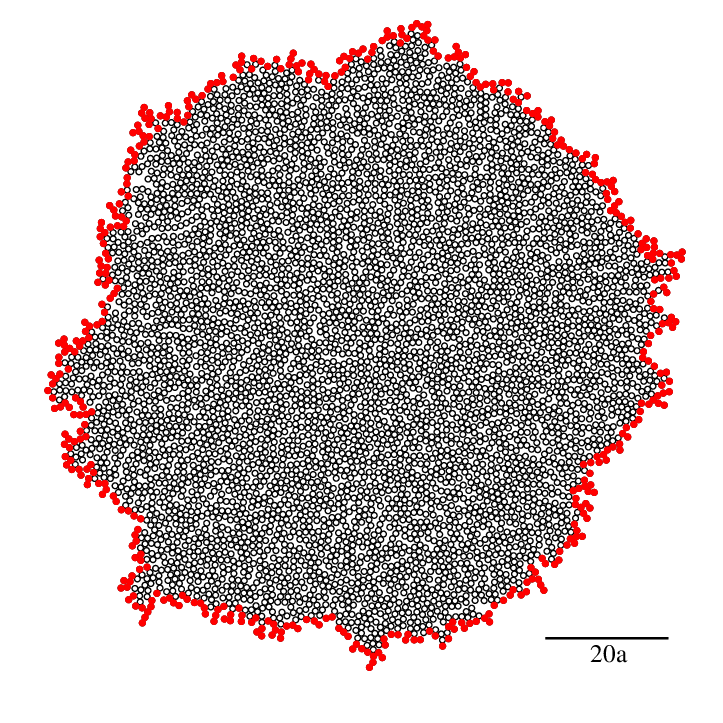
Image credit: Silvio Costa Ferraria et al - Figure 1 from Pitfalls on the determination of the universality class of radial clusters
Created by Murray Eden in 1961 (paper (PDF)), this is a type of surface fractal growth process where material randomly accumulates on the boundary of clusters. Sort of like DLA but without all the empty space between branches. Thought to be a good way to model certain kinds of bacterial and lichen growth.
Algorithm at a glance:
* indicates a potential simulation parameter
Key terms:
Articles:
Code projects:

[!NOTE] Related to Primordial Particle System and agent-based modelling.
Image credit: detail of the example results from Particle Life Simulation by Hunar Ahmad
Family of particle systems in which every particle belongs to one of several types (usually drawn as colors), and every ordered pair of types is assigned its own attraction or repulsion strength. Those strengths are held in a small matrix that can be filled randomly and then tuned by hand, which makes the system extremely easy to explore - each new matrix is effectively a new set of "physics" to play with.
Crucially, the matrix does not have to be symmetric: green can be attracted to red while red is repelled by green. That asymmetry is what lifts the results beyond simple clumping, producing cell-like clusters with membranes, wandering "creatures" that chase and flee each other, orbiting pairs, snaking chains, and blobs that pinch off copies of themselves - all within one parameter space.
Originally explored by Jeffrey Ventrella as Clusters and later popularized under the name "Particle Life" by CodeParade in 2018, this is one of the most approachable emergent systems to implement, since the core is just a nested loop over pairs of particles.
Not to be confused with the Primordial Particle System, which uses a single kind of particle steering by neighbor counts - here the effects depend entirely on multiple types treating each other differently.
Algorithm at a glance:
* indicates a potential simulation parameter
k* types (colors).k × k matrix* of attraction values (commonly in the range -1 to 1), one for each ordered pair of types, where negative values mean repulsion. Random matrices are a good starting point, and the matrix need not be symmetric.Key terms:
k × k table of per-pair attraction and repulsion strengthsArticles:
Videos:
Projects:

Image credit: Sage Jenson (@mxsage)
Technique for modelling the observed behaviors of the slime mold physarum polycephalum using agent-based modelling. Originally described in 2010 paper by Jeff Jones, and more recently popularized by artist Sage Jensen (@mxsage), this algorithm produces highly dynamic and organic-looking webs that can seem very life-like and biological in nature.
Algorithm at a glance:
* indicates a potential simulation parameter
Articles:
Code projects:
Creative projects:

[!NOTE] Related to Particle Life and agent-based modelling.
Image credit: detail of Figure 3G from Schmickl, Stefanec & Crailsheim (2016)
Described in 2016 by Thomas Schmickl, Martin Stefanec and Karl Crailsheim of the Artificial Life Lab in Graz, Austria, a Primordial Particle System (PPS) is a minimal agent-based model in which self-propelled particles move through continuous space while steering based only on how many neighbors they can see to their left and right - a motion law even simpler than boids, with no cohesion, separation or alignment rules. It is a separate system from Particle Life, where all of the behavior comes instead from multiple particle types with per-pair attraction rules.
Despite containing no notion of cells, membranes or reproduction, the system spontaneously produces cell-like structures with a dense interior surrounded by a ring-like membrane, and those structures go through a full life cycle: they feed on the surrounding "nutrient" field of free particles, grow, divide into daughter cells and spores, and die when starved. Left running, the population of cells levels off along a sigmoidal curve much like bacteria growing in a petri dish, making this one of the most striking demonstrations of how self-structuring, self-reproducing and self-sustaining behaviors can emerge from a single line of math.
Motion law:
$$\Delta\phi = \alpha + \beta \cdot N_{t,r} \cdot \text{sign}(R_{t,r} - L_{t,r})$$
Where $L$ and $R$ are the number of neighbors within radius $r$ in the semicircles to the particle's left and right, $N = L + R$ is the total number of neighbors, $\alpha$ is a fixed rotation, $\beta$ is a rotation proportional to local crowding, and a positive $\Delta\phi$ is a turn to the right.
Algorithm at a glance:
* indicates a potential simulation parameter
Reference parameter set: $\text{PPS} = \langle r = 5, \alpha = 180°, \beta = 17°, v = 0.67 \rangle$
Color coding (as used in the paper):
Articles:
Videos:
Projects:

[!NOTE] Related to convolution kernel and Laplace equation.
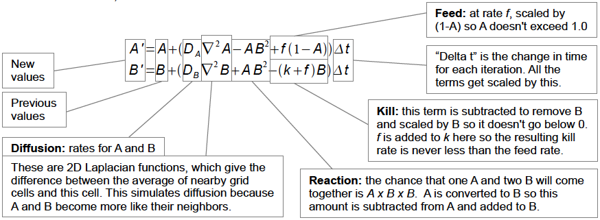
Grid-based process that generates complex and dynamic patterns based the interactions of two chemicals as they diffuse through a medium and react with one another. At every location on the grid these chemicals (usually referred to as A and B) have a chance of causing a reaction that converts chemicals of one type to another based on their relative concentrations at that location.
Throughout the simulation chemical A is added at a particular feed rate (f) and chemical B is removed at a particular kill rate (k) - adjusting these rates can result in wildly different emergent patterns.
Equation (via Karl Sims):
Key terms:
A is added to systemB is removed from the systemA will be converted to a B when in the presence of two Bs.Articles:
Notable tools:
Code projects:
Creative projects:
Videos:

Process for iteratively growing networks of branching lines based on the distribution of growth hormone sources (called "auxin" sources) to which the lines are attracted. Originally described by Adam Runions and collaborators at the Algorithmic Botany group at the University of Calgary, this system can be used to simulate the growth of leaf venation patterns and tree-like structures, as well as many other vein-like systems like Gorgonian sea fans, circulatory systems, root systems, and more.
The original algorithm describes methods for generating both "open" (as seen in the example GIF) and "closed" venation networks, referring to whether or not secondary or tertiary veins connect together to form loops (or anastomoses).
Algorithm at a glance:
For both the open and closed variants of this algorithm, begin by placing a set of points on the canvas representing sources of either the auxin growth hormone (as in leaves) or ambient nutrients (as in trees).
Open venation:
Closed venation:
Auxin flux canalization:
Key terms:
Articles and papers:
Creative projects:
Code projects:
Videos:

String rewriting system invented by biologist Aristid Lindenmayer in 1968 to model the growth processes of plant development and other organisms. L-systems use simple grammatical rules to iteratively expand a string of symbols, which can then be interpreted geometrically (e.g., using turtle graphics) to produce complex branching structures. Despite their simplicity, L-systems can generate remarkably naturalistic plant forms, fractals, and branching patterns.
The key insight is that local production rules (each symbol rewrites to a sequence of symbols) applied recursively across iterations can generate globally complex structures without explicitly encoding the final form. This makes L-systems particularly powerful for modeling hierarchical biological growth.
Algorithm at a glance:
* indicates a potential simulation parameter
F (move forward and draw), f (move forward without drawing), + (turn left), - (turn right), [ (push position/heading to stack), ] (pop position/heading from stack)Example:
| Description | Rendered Result |
|---|---|
Axiom: FRule: F → F[+F]F[-F]FAfter iteration 1: F[+F]F[-F]FAfter iteration 2: F[+F]F[-F]F[+F[+F]F[-F]F]F[+F]F[-F]F[-F[+F]F[-F]F]F[+F]F[-F]FWhen rendered with angle=25°, this produces a branching plant-like structure. |  |
Key terms:
Articles:
Videos:
Notable tools and libraries:

[!NOTE] Related to reaction-diffusion.
Physical process by which a homogeneous mixture (a molten alloy, polymer blend, glass, etc.) spontaneously separates into two distinct phases when rapidly cooled ("quenched") into an unstable region of its phase diagram. Unlike typical nucleation-based phase separation, no discrete starting sites or thermodynamic barrier are needed - tiny composition fluctuations grow everywhere in the material simultaneously.
The result is a characteristic pattern of intertwined, worm-like regions that grow and merge ("coarsen") over time while roughly maintaining the same overall proportions of each phase - visually similar to some reaction-diffusion patterns, though it arises from a different underlying process (phase-separation thermodynamics rather than a chemical feed/kill reaction). It's commonly modeled with the Cahn-Hilliard equation, a PDE describing how the concentration of the two phases diffuses and separates over time.
Algorithm at a glance:
* indicates a potential simulation parameter
Key terms:
Articles:
Code projects:

[!NOTE] Related to polyhedra and Platonic solids.
Set of 13 semi-regular convex polyhedra composed of regular polygons meeting in identical vertices, excluding the 5 Platonic solids (which are composed of only one type of polygon) and excluding the prisms and antiprisms.
Each shape can be constructed by starting with one of the Platonic solids and truncating it's corners or edges in various ways.
List of Archimedean solids:
| Name | Faces | Edges | Vertices | Image |
|---|---|---|---|---|
| Truncated tetrahedron | 4 triangles 4 hexagons | 18 | 12 |  |
| Cuboctahedron | 8 triangles 6 squares | 24 | 12 |  |
| Truncated cube | 8 triangles 6 octagons | 36 | 24 |  |
| Truncated octahedron | 6 squares 8 hexagons | 36 | 24 |  |
| Rhombicuboctahedron | 8 triangles 18 squares | 48 | 24 |  |
| Truncated cuboctahedron | 12 squres 8 hexagons 6 octagons | 72 | 48 |  |
| Snub cube | 32 triangles 6 squares | 60 | 24 |  |
| Icosidodecahedron | 20 triangles 12 pentagons | 60 | 30 |  |
| Truncated dodecahedron | 20 triangles 12 decagons | 90 | 60 |  |
| Truncated icosahedron | 12 pentagons 20 hexagons | 90 | 60 |  |
| Rhombicosidodecahedron | 20 triangles 30 squares 12 pentagons | 120 | 60 |  |
| Truncated icosidodecahedron | 30 squares 20 hexagons 12 decagons | 180 | 120 |  |
| Snub dodecahedron | 80 triangles 12 pentagons | 150 | 60 |  |
Articles:
Videos:

[!NOTE] Related to convolution kernel.
A regular grid of cells with states that are updated each iteration in according to rules. Developed by Stanislaw Ulam and John von Neumann at the Los Alamos National Laboratory in the 1940s, this system has been used to model physical, biological, and social phenomena with remarkable variety and accuracy.
Key terms:
Types:
[0,9], then a cell with value 2 can be "consumed" by a neighboring cell with value 3, causing the cell to take on the value of 3. When cells reach the state at the end of the range, they are reset to the state at the beginning of the range (wrapping around).t, you can compute the state at t - 1.t depends on the state at both t - 1 and t - 2.Wolfram's classification:
Stephan Wolfram defined four classes that can be used to describe any cellular automaton or other simple computational model based on their observed behaviors. These definitions are qualitative in nature, with some room for intepretation, but are nonetheless considered the most effective classification scheme that currently exists for cellular automata.
Well-known rules and rule families:
Articles, books, and other writings:
Code projects:
Creative projects:
Notable software:

[!NOTE] Related to polyhedra, Platonic solids, and Archimedean solids.
Conway polyhedron notation, invented by mathematician John Horton Conway and later extended by George W. Hart, is a compact system for describing complex polyhedra as a short chain of operators applied to a simple seed shape. Operators are single lowercase letters applied right-to-left, so taC means "start with a cube (C), apply ambo (a), then truncate (t)" - the same recipe that produces a truncated cuboctahedron. This turns a huge space of polyhedra into a small, composable vocabulary, which is why it's a popular basis for procedural polyhedron tools.
Seeds:
Starting shapes are abbreviated with a single capital letter: T (tetrahedron), C (cube), O (octahedron), D (dodecahedron), I (icosahedron), Pn (n-gonal prism), An (n-gonal antiprism), Yn (n-gonal pyramid).
Core operators:
d (dual) - swaps every face for a vertex and vice versa (e.g. dC = octahedron).a (ambo) - adds a vertex at the midpoint of every edge and connects them, producing the "rectified" Archimedean forms (e.g. aC = cuboctahedron).t (truncate) - slices off each vertex, turning it into a small new face.k (kis) - raises a pyramid on every face by adding a vertex at its center.j (join) - connects the centers of adjacent faces, replacing them with quadrilaterals.e (expand) - pushes each face outward along its normal and fills the resulting gaps with new faces.s (snub) - like expand, but with a twist added, producing a chiral form with extra triangular faces (e.g. sC = snub cube).g (gyro) - the dual of snub; introduces a chiral twist without adding triangles.b (bevel) - combines truncation and ambo.o (ortho) - subdivides each face into quadrilaterals around its center.m (meta) - combines kis and join.George Hart later added r (reflect, mirrors a chiral form) and p (propellor), and modern implementations support dozens more (chamfer, needle, zip, loft, whirl, and others).
Articles:
Notable tools:
conway by Adrian Rossiter and Roger Kaufman - command-line Conway notation processor, adapted from Hart's original implementation[!NOTE] Related to cellular automata, reaction-diffusion, noise, and image processing.
A convolution kernel is a small matrix of numbers that defines a weighted neighborhood operation. When applied to a grid (like an image, scalar field, or cellular grid), the kernel is placed over each location, its values are multiplied by the overlapping grid values, the products are summed, and the result is written to the center cell. This operation is the foundation for countless techniques across image processing, simulations, and signal analysis.
The kernel acts as a filter that emphasizes or suppresses patterns in the data. A kernel of all ones computes the sum of a neighborhood. A kernel with larger values in the center and smaller values at the edges acts as a blur (weighted average). Kernels with opposing signs can detect edges. Different kernels solve different problems, but they all follow the same convolution process: slide, multiply, sum, repeat.
Core concepts:
Applications across domains:
Articles:
Videos:
Code projects and libraries:

[!NOTE] Related to Chladni plate
Study of the visible effects of sound and vibration on physical media. Typically involves the vibration of a plate or membrane onto which fine powder or fluids have been placed, which subsequently arrange themselves into highly symmetrical, complex patterns based on the intensity of displacement of various regions of the vibrating plate. Areas that are moving a lot will "kick" material away from them while areas that are moving very little allow material to settle and accumulate. These areas of relatively little vibration are caused by destructive interference of waves as they propagate across the plate/membrane and become out of phase with one another, creating "dead zones" where these waves cancel each other out.
Articles:
Creative projects:

[!NOTE] Related to tiling / tessellation.
Delaunay triangulation is a way of connecting a set of points to form a network of non-overlapping triangles. One of the key properties of Delaunay triangulations is that the circumcircles associated with each triangle contains no other points than their three triangle vertices. When extended into 3D, Delaunay triangulation is useful for creating meshes.
Voronoi diagrams are the dual of Delaunay triangulations. This means that once a Delaunay triangulation has been computed for a set of points, a Voronoi diagram can be drawn without any additional data - just draw lines connecting the centers of the circumcircles!
Voronoi diagrams are very useful for efficiently and organically partitioning (splitting up) both 2D and 3D space. They are especially good for accurately modelling the way soft bodies (like biological cells) get smushed together in constrained environments, like embryonic cells undergoing mitosis.
Voronoi diagrams are often used (perhaps overused) in digital fabrication applications, especially 3D printing, for their characteristic aesthetic style and their ability to reduce material usage while preserving overall form. Given their popularity among amateur 3D printing enthusiasts, this effect is probably best used sparingly in serious applications.
Articles:

[!NOTE] Related to Golden ratio.
Sequence of numbers in which each number is the sum of it's two preceding numbers. Binet's formula shows that the ratio of two consecutive numbers tends towards the golden ratio as the sequence progresses. Fibonacci numbers appear unexpectedly often in biology, having been observed in branching of trees, the arrangement of leaves on a stem, the fruit sprouts of a pineapple, the flowering of an artichoke, an uncurling fern and the arrangement of a pine cone's bracts.
Formula:
$$F_{0}=0,\quad F_{1}=1,$$
$$F_{n}=F_{n-1}+F_{n-2},$$
Sequence begins with:
$$(0), 1, 1, 2, 3, 5, 8, 13, 21, 34, 55, 89, 144, \ldots$$
Articles:

Series of sinusoidal wave functions that get added together to generate a different, more complex function. In the context of morphogenesis (form generation), any line drawing can be "deconstructed" into a series of arc segments which can in turn be represented by a series of circles whose radii and rotation speeds correspond to the radii and lengths of the arc segments.
Fourier series and Fourier transforms are deeply mathematical topics with applications and research far beyond the scope of this resource list. They are extremely useful in the field of digital signal processing for noise reduction, compression, audio analysis, and so much more. A very well-known algorithm known as the fast Fourier transform (FFT) enables extraction of waveforms from music for the purposes of audio visualization.
Articles:
Videos:

Infinitely complex patterns generated via recursion that are self-similar across all scales. Thought to be found in abundance in nature, though "true" (infinite) fractals are not possible because nature uses physical matter, which has particular structures at the microscopic and smaller scales (molecules, atoms, elementary particles, etc).
Fractal features can be observed in nature in tree branching structures, leaf veins, terrain, surface textures, coastlines, rivers, succulents, snowflakes, rivers, lightning bolts, nautilus shells (both form and pattern), and so much more.
Key terms:
Notable fractals:
Articles:
Notable software:
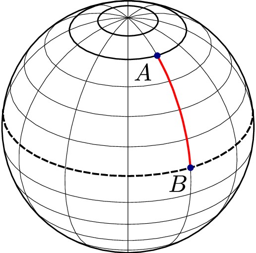
Image credit: Vikash Mittal - Geometric phase and its applications: topological phases, quantum walks and non-inertial quantum systems (FIGURE 2).
The shortest path between two points on a curved surface - a generalization of the concept of a "straight line" to curved geometry. On a flat plane a geodesic is just a straight line; on the surface of a sphere, geodesics are arcs of great circles; on more complex curved surfaces they can bend and twist while still remaining locally "as straight as possible" at every point.
Related terms:
Articles:

[!NOTE] Related to geodesics, Platonic solids, and polyhedra.
Spherical shell structure of triangular struts whose vertices all lie on a circumscribed sphere. It's typically derived from a Platonic solid with triangular faces (usually an icosahedron) by subdividing each face some number of times (the dome's "frequency") and projecting the new vertices onto the sphere - higher frequencies mean more, smaller struts and a closer approximation of a sphere.
Named for the geodesic - the shortest path between two points on a curved surface - since its edges approximate great-circle arcs. The shell distributes structural stress evenly, giving it a high strength-to-weight ratio. Popularized (though not invented) by Buckminster Fuller, whose name was later borrowed for the similarly-shaped carbon molecules called buckminsterfullerenes.
Key terms:
nV (e.g. 3V), where a higher number means smaller, more numerous struts.Articles:
Notable software:
Notable real-world geodesic domes:

[!NOTE] Related to the golden ratio and phyllotaxis.
Radial version of the golden ratio. It is the smaller of the two angles created by sectioning the circumference of a circle according to the golden ratio; that is, into two arcs such that the ratio of the length of the smaller arc to the length of the larger arc is the same as the ratio of the length of the larger arc to the full circumference of the circle.
In degrees the angle is approximately 137.5077640500 ..., or just 137.5 for brevity.
Articles:
Creative projects:

[!NOTE] Related to the Fibonacci sequence.
Also expressed as the Greek letter phi (φ), this irrational number pops up when the ratio of two numbers is the same as the ratio of their sum to the largest of the two numbers. It has been observed in many fields of the natural sciences at every scale and is has become associated with aesthetic beauty, giving it a nearly mythic reputation for some.
| Expressed algebraicly | $\varphi = \frac{1 + \sqrt{5}}{2} = 1.6180339887\ldots$ |
| Expressed as line segments | 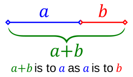 |
Articles:

A surface defined by an equation in the form of 
Examples of implicit surface equations:
| Plane | $x+2y-3z+1=0$ |
| Sphere | $x^{2}+y^{2}+z^{2}-4=0$ |
| Torus | $(x^{2}+y^{2}+z^{2}+R^{2}-a^{2})^{2}-4R^{2}(x^{2}+y^{2})=0$ |
| Surface of genus 2 | $2y(y^{2}-3x^{2})(1-z^{2})+(x^{2}+y^{2})^{2}-(9z^{2}-1)(1-z^{2})=0$ |
| Surface of revolution | $x^{2}+y^{2}-(\ln(z+3.2))^{2}-0.02=0$ |
Articles:
Notable software:

Equations used to calaculate the positions of a series of rigidly-linked segments (called the kinematic chain) based on the location of the end effector, usually located at the tip of the last segment. Useful for robotic systems like drawing machines, robot arms, and more.
Inverse kinematics calculate the angles of each linked segment given the desired location of the end effector. Will give you the angles of each segment, which can in turn be converted into motor positions for a robot.
Forward kinematics calculate the location of the end effector given the angles and lengths of each linked segment.
Articles:
Videos:

[!NOTE] Related to DLA, DBM, Saffman–Taylor instability, reaction-diffusion, minimal surface, fluid simulation, and Laplace transform.
The Laplace equation, $\nabla^2 \varphi = 0$, says that a field's value at any point equals the average of its immediate surroundings - no interior point can be a local bump or dip. It shows up constantly in physics because it's simply the steady-state form of diffusion, heat flow, and potential fields: whenever something free to spread out (heat, concentration, charge, pressure) has finished settling, its value obeys this equation. Solutions are called harmonic functions.
That abstractness is exactly why it matters for morphogenesis: several branching growth patterns already covered elsewhere in this list are, mathematically, the same equation wearing different clothes - a family of processes collectively known as Laplacian growth.
Laplacian growth - from equation to organic form:
Each of these solves the Laplace equation in the region around a growing cluster, then advances the cluster's boundary fastest wherever the resulting field's gradient is steepest:
This is why DLA clusters, electrical discharge patterns, and viscous fingers all look so similar despite arising from unrelated physics - they're all boundaries growing into a harmonic field, differing only in their noise and boundary conditions.
Key terms:
Articles:
Videos:
Code projects:
[!NOTE] Related to Laplace equation
Mathematical transform that converts a function of time into a function of complex frequency, turning differential equations into algebraic ones that are often easier to solve. It is widely used in engineering, physics, and control theory to analyze dynamic systems and their stability, resonance, and response.
The Laplace transform maps a time-domain function $f(t)$ to a frequency-domain function $F(s)$. In this form, differentiation becomes multiplication and convolution becomes multiplication, making many system problems easier to analyze. Its inverse recovers the time-domain solution for applications such as growth dynamics, signal propagation, and feedback-driven behavior.
Definition:
$$F(s) = \mathcal{L}{f(t)} = \int_0^{\infty} e^{-st} f(t) , dt$$
Where $s = \sigma + i\omega$ is a complex frequency variable, $t$ is time, and the integral converges for sufficiently large $\sigma$.
Key properties:
| Property | Formula | Description |
|---|---|---|
| Linearity | $\mathcal{L}{af(t) + bg(t)} = a\mathcal{L}{f(t)} + b\mathcal{L}{g(t)}$ | Sum transforms equal sum of transforms |
| Differentiation rule | $\mathcal{L}{f'(t)} = sF(s) - f(0)$ | Converts derivatives to algebraic operations |
| Integration rule | $\mathcal{L}{\int_0^t f(\tau),d\tau} = \frac{F(s)}{s}$ | Converts integrals to division by $s$ |
| Convolution theorem | $\mathcal{L}{f(t) * g(t)} = F(s)G(s)$ | Converts convolution to multiplication |
| Final value theorem | $\lim_{t \to \infty} f(t) = \lim_{s \to 0} sF(s)$ | Determines steady-state behavior |
| Initial value theorem | $f(0^+) = \lim_{s \to \infty} sF(s)$ | Determines initial conditions |
| Frequency shifting | $\mathcal{L}{e^{at}f(t)} = F(s-a)$ | Scaling exponential shifts frequency |
| Time shifting | $\mathcal{L}{f(t-a)u(t-a)} = e^{-as}F(s)$ | Delay in time domain multiplies by $e^{-as}$ |
Key terms:
Articles:
Also known as Bowditch curves, these figures plot the trajectories of a point as it follows the path of two simultaneous sinusoidal motions.
Can be created using various physical systems including oscilloscopes, harmonographs, and more.
Equations:
$$x = a \sin t,\quad y = b \sin(nt + \varphi)$$
$$0 \leq \varphi \leq \frac{\pi}{2}, \quad n \geq 1$$
Articles:
Videos:

[!NOTE] Related to soft-body physics, cloth simulation, Verlet physics, and physics engines.
A mass-spring system is a general mathematical model for deformable bodies: a graph of point masses connected by springs that obey Hooke's law (restoring force proportional to displacement from a rest length). It's one of the oldest and most widely reused abstractions in computational physics, showing up not just in computer graphics but in structural engineering (truss analysis), molecular dynamics (bond modeling), and biomechanics (tissue and muscle models). Its appeal is that a small number of local rules - distance constraints and simple forces - can produce believable global deformation without solving a full continuum mechanics problem.
In graphics and simulation, mass-spring systems are the conceptual backbone of cloth simulation, rope/hair simulation, and soft-body deformation, and are typically stepped forward with Verlet integration for stability. Real-time applications commonly layer three kinds of springs to control different deformation modes: structural springs (resist stretching), shear springs (resist skewing), and bend springs (resist folding).
Algorithm at a glance:
* indicates a potential simulation parameter
F = stiffness × (current_distance - rest_length).F_damping = damping × relative_velocity.Key terms:
Articles:
Code projects:
Videos:

The medial axis is sort of like the "skeleton" of a shape. It consists of a set of lines and curves upon which every point is equidistant between at least one closest point on the shape's boundary. In 2D this skeleton can also be thought of as a set of lines/curves whose points are the centers of circles that are tangent to at least two points on the shape's boundary.
Has applications in computer vision, pose estimation, 2D/3D character rigging, architecture, BIM (escape route optimization), and more.
Related terms:
Articles:
Notable Tools:

[!NOTE] Related to Laplace equation.
A minimal surface is a surface that locally minimizes area, which means it settles into the smallest possible shape for a given boundary while keeping its mean curvature equal to zero. Minimal surfaces show up in architecture, material design, geometry, and optimization, and they are useful whenever you want a smooth surface or membrane that uses as little area as possible.
A soap film stretched across a wire frame is the classic physical example: the film naturally relaxes into a shape that balances tension everywhere. Frei Otto's soap-bubble experiments were important for showing how these forms emerge in the real world.
Equations:
| Equation | Explanation |
|---|---|
| $H = (k_1 + k_2) / 2 = 0$ Where: $H$ = mean curvature (the average curvature of a surface); $k_1$ and $k_2$ = principal curvatures (the two main curvatures at a point). | The minimal surface condition says the average of the principal curvatures is zero. |
| $\nabla \cdot \left(\frac{\nabla u}{\sqrt{1 + \lvert\nabla u\rvert^2}}\right) = 0$ Where: $u(x, y)$ = surface height; $\nabla u$ = gradient of the surface; $\nabla \cdot$ = divergence (how much a field spreads out or converges). | The minimal surface equation is the graph form of a minimal surface. |
| $A[u] = \iint \sqrt{1 + u_x^2 + u_y^2},dx,dy$ Where: $A[u]$ = area functional (the formula that computes total area); $u_x$ and $u_y$ = partial derivatives of the surface height. | The area functional gives the total surface area. |
Key terms:
Examples:
| Term | Equation |
|---|---|
| Catenoid | $r = a \cosh\left(\frac{z}{a}\right)$ |
| Helicoid | $x = u \cos v, \quad y = u \sin v, \quad z = a v$ |
| Gyroid | $\sin x \cos y + \sin y \cos z + \sin z \cos x = 0$ |
Articles:
Notable software:
Notable creative work:
Notable real-world buildings:
Natural phenomena:

Class of optimization problems that involve determining efficient ways to arrange (pack) objects into containers. Packing problems can be tackled using discrete mathematical methods, physics systems (as seen in Nervous System's Kinematics series), and even genetic algorithms and machine learning.
Has major applications in digital fabrication, manufacturing, and shipping logistics where material and space usage is directly related to costs. In 2D, packing/nesting problem solutions are useful for minimizing waste material in sheet goods like plywood and sheet steel, even for hobbyists. In 3D these solutions are useful for fitting as many objects as possible into 3D printer build envelopes (see article from Sculpteo).
Related terms:
Articles:
Notable tools:
Videos:

Mathematical framework that studies the behavior of connected clusters in random networks. At its core, percolation explores the threshold at which a system transitions from isolated fragments to a connected network spanning the entire space - a critical phenomenon with applications in material science, epidemiology, network analysis, and growth simulation.
The classical model places sites or bonds randomly on a grid, each with some occupation probability $p$. As $p$ increases, small disconnected clusters begin to merge and grow. At a critical threshold $p_c$ (the percolation threshold), a “giant component” suddenly emerges that connects from one side of the system to the opposite side. Above the threshold, clusters merge rapidly; below it, they remain fragmented. This sharp transition is a classic example of a phase transition in physics.
Key concepts:
Percolation can model porous media (oil migration through rock), disease spread (how infections propagate through a population), forest fires (how rapidly fires spread through dense vegetation), and network robustness (how many nodes can fail before connectivity is lost). In the context of morphogenesis, percolation-based growth can generate branching patterns, fragmented structures, and networks with natural-looking interconnectivity.
Articles:
Code projects and interactive tools:

[!NOTE] Related topics include the golden ratio, the golden angle, and the Fibonacci sequence.
Refers to the arrangement (taxis) of leaves (phyllo) on a plant stem. Also can refer to seed arrangements and succulent geometry.
Types:
Articles:
Code projects:
Videos:

[!NOTE] Related to polyhedra and Archimedean solids.
Set of regular, convex polyhedra constructed using congruent, regular polygonal faces with the same number of faces meeting at each vertex. Euclid (and perhaps Theaetetus proved mathematically that there are only five shapes that fit this criteria (below).
| Name | Polygon type | Faces | Edges | Vertices | Image |
|---|---|---|---|---|---|
| Tetrahedron | Triangle | 4 | 6 | 4 |  |
| Cube | Square | 6 | 12 | 8 |  |
| Octahedron | Triangle | 8 | 12 | 6 |  |
| Dodecahedron | Pentagon | 12 | 30 | 20 |  |
| Icosahedron | Triangle | 20 | 30 | 12 |  |
Articles:
Videos:

[!NOTE] Related to Platonic solids, Archimedean solids, geodesic domes, and Conway operators.
A polyhedron is a solid bounded by flat polygonal faces, straight edges, and sharp vertices - the Platonic and Archimedean solids are just the two best-known families in a much larger space of shapes. For generative artists, polyhedra are a useful design space precisely because they're so constrained: a handful of construction rules (regular faces, identical vertices, symmetric arrangements) generate a finite, well-catalogued set of "correct-looking" forms, which is why the same few solids keep reappearing as base meshes for subdivision, geodesic domes, and procedural modeling more broadly.
Key concepts:
Major classes:
Symmetry:
A shape has symmetry when it can be rotated or reflected and still look exactly the same - spin a cube 90° around an axis through two opposite faces and you can't tell it moved. The full set of ways a shape can do this is called its symmetry group, and the larger it is, the more interchangeable the shape's faces, edges, and vertices look.
Highly symmetric polyhedra fall into just three of these groups (doubled again with mirror reflections) - part of why the same few base shapes keep recurring in generative work:
A polyhedron's symmetry group also determines whether every vertex looks like every other vertex (isogonal, true of the Platonic and Archimedean solids), every face looks like every other face (isohedral, true of the Platonic and Catalan solids), or every edge looks like every other edge (isotoxal).
Stellation and facetting:
These are dual, opposite operations for generating new polyhedra from existing ones:
Key terms:
V - E + F = 2 for any simple convex polyhedron; a quick sanity check for procedurally generated meshes.{p, q} describing a regular polyhedron by its face polygon (p-gon) and how many meet at each vertex (q); star polyhedra use fractions, e.g. {5/2, 5} for the small stellated dodecahedron.Articles:
Videos:
Notable tools:
Code projects:

[!NOTE] Related to DBM, DLA, differential growth, reaction-diffusion, fluid simulation, Hele-Shaw cells, and Laplace equation
Also known as viscous fingering, this is a fluid dynamics instability that occurs at the interface between two fluids of different viscosity when a less viscous fluid is pushed into a more viscous one - inside a narrow gap such as a Hele-Shaw cell, or through a porous medium. Rather than advancing as a flat front, the interface spontaneously breaks up into branching, finger-like intrusions.
The instability is a positive feedback loop: any small bump that forms on the interface sits in a region of lower flow resistance, so it advances faster than its surroundings, growing further ahead and widening into a finger; the same feedback then acts along the flanks of that finger, splitting its tip and producing a branching structure reminiscent of diffusion-limited aggregation and the dielectric breakdown model. Interfacial tension between the two fluids counteracts this, damping out short-wavelength wrinkles and setting a characteristic finger width - the balance between the two effects selects the fairly regular finger spacing seen in real experiments.
Key terms:
DIY experiments:
Viscous fingering can be observed with everyday materials without specialized equipment. When two surfaces are slowly peeled or pulled apart with a thin viscous layer (honey, jam, corn syrup, or hand lotion) between them, the less viscous fluid (air) displaces the viscous layer, creating fingerlike flow patterns at the retreating interface. The same effect occurs in setups such as:
These "peeling" setups exhibit viscous fingering because the viscous fluid resists the air's advance, creating an unstable interface that spontaneously breaks into fingers. This is closely related to the lifted Hele-Shaw cell concept—in both cases, viscous resistance shapes fluid interfaces during separation or displacement, revealing the same underlying physics.
Articles:

[!NOTE] Related to Fourier series
Spherical harmonics are a set of special functions defined on the surface of a sphere that form a complete, orthonormal basis - meaning any reasonably well-behaved function over the sphere (e.g. a bumpy radius, a lighting environment, a temperature field) can be reconstructed as a weighted sum of them, in the same way a Fourier series reconstructs a periodic signal from sines and cosines. They arise naturally as the angular part of the solution to Laplace's equation in spherical coordinates, which is why they show up throughout physics wherever spherical symmetry is involved - gravitational and electric potentials, atomic orbitals, geodesy, and the cosmic microwave background.
Each spherical harmonic is indexed by a degree $l$ and an order $m$, and looks like a pattern of positive and negative lobes tiling the sphere; low-degree harmonics vary slowly across the surface (capturing broad, low-frequency features) while higher-degree harmonics oscillate more rapidly (capturing fine detail) - directly analogous to how low vs. high frequency terms behave in a Fourier series. This makes them a useful tool for morphogenesis and shape modeling: an arbitrary blob-like or organic 3D form can be approximated, generated, or smoothly deformed by manipulating just a handful of spherical harmonic coefficients instead of a dense mesh.
Key terms:
Articles:
Code projects and tools:
pyshtools) - library for spherical harmonic transforms, spectral analysis, and working with gravity/magnetic/topography field data.
Trajectories of deterministic dynamical systems that exhibit chaotic behavior while remaining confined within a bounded region of space. Unlike ordinary attractors (fixed points or periodic cycles), strange attractors have a fractal structure with infinite detail and display sensitive dependence on initial conditions - tiny differences in starting state lead to wildly divergent outcomes. Despite their deterministic rules, the long-term behavior appears random or turbulent.
Strange attractors emerge in nonlinear systems where feedback loops create complex dynamics. They are "strange" because they combine order (the system never leaves a bounded region) with chaos (unpredictable behavior). They are "attractors" because trajectories from nearby initial conditions are pulled toward them over time. Their fractal dimension is typically non-integer, a hallmark of their geometric complexity.
Strange attractors have been observed in fluid dynamics (turbulence), weather systems (weather chaos), population dynamics, electronic circuits, and more. In generative art and morphogenesis, they are often used to create organic-looking, intricate patterns and forms that would be difficult or impossible to design by hand. The self-similar, fractal-like structures they produce can simulate natural phenomena like cloud formations, terrain, and biological branching patterns.
Key terms:
Notable attractors:
Articles:

Also known as the Lamé curve, this equation describes a closed curve that can generate shapes that look like pinched or inflated ellipses. At the extremes of the parameter space the shapes can range from an outline of a plus (+) symbol to a nearly rectangular shape with rounded corners.
Equations:
| General form | $\left|\frac{x}{a}\right|^{n} + \left|\frac{y}{b}\right|^{n} = 1$ |
| Parametric | $x(t)=\pm a\cos^{\frac{2}{n}}t,\quad y(t)=\pm b\sin^{\frac{2}{n}}t,\quad 0\leq t\leq\frac{\pi}{2}$ |
Articles:
Videos:

Generalized version of the superellipse formula proposed by Johan Giellis around 2000, capable of far more variety than the original superellipse. Unfortunately, Johan has patented use of the formula (via his company Genicap) in both the US and the EU, which means you should avoid using it for any kind of commercial work, or work that could be commercialized in some way later.
The superformula can be used to generate both 2D and 3D forms. To create 2D forms, use the general form equation to obtain polar coordinates that can be converted into Cartesian coordinates for drawing on a screen. To create 3D forms, compute the polar coordinates for two 2D supershapes, then "mix" them together using the 3D equations below.
Equations:
| General form | $r(\varphi) = \left(\left|\frac{\cos(m_1\varphi/4)}{a}\right|^{n_2} + \left|\frac{\sin(m_2\varphi/4)}{b}\right|^{n_3}\right)^{-1/n_1}$ |
| 3D equations | $x=r_1(\theta)\cos\theta\cdot r_2(\varphi)\cos\varphi,\quad y=r_1(\theta)\sin\theta\cdot r_2(\varphi)\cos\varphi,\quad z=r_2(\varphi)\sin\varphi$ |
Where r is a radius and φ (phi) is an angle.
Where φ (latitude) varies between −π/2 and π/2 and θ (longitude) between −π and π.
Articles:
Code projects:
Videos:

[!NOTE] Related to polyhedra, Wave Function Collapse (WFC), and Delaunay triangulation and Voronoi diagrams.
A tiling (or tessellation) is a covering of a plane, or other surface, by one or more shapes ("tiles") with no gaps and no overlaps. Like polyhedra, tilings are a design space defined by a small set of construction rules, which makes them a reliable source of "correct-looking" repeating patterns for generative art, procedural texture generation, and physical fabrication (laser-cut panels, tiled floors, quilting).
Key concepts:
Notable named tilings:
Key terms:
3.6.3.6 for a triangle-hexagon-triangle-hexagon arrangement.Articles:
Videos:
Notable tools:
Code projects:

Asks the question "Given a list of cities and the distances between each pair of cities, what is the shortest possible route that visits each city and returns to the origin city?" This classic problem is computer science classrooms to teach algorithm design and optimization techniques.
Useful for creating single-line drawings for use with pen plotters, laser cutters, CNC machines, and more.
Articles:
Notable software:

[!NOTE] Related to physics engines and particle systems.
Image credit: Matthew Fisher - Cloth
Family of numerical integration methods for simulating motion that skip storing velocity explicitly, instead deriving it implicitly from a particle's current and previous position. Named after French physicist Loup Verlet, who used it for molecular dynamics simulations in the 1960s, though the technique dates back further.
At each step, a particle's next position is calculated from its current position, its previous position, and the acceleration currently acting on it:
newPosition = 2 * currentPosition - previousPosition + acceleration * timeStep^2
Because positions - not velocities - are what's being directly manipulated, distance constraints (like the fixed-length "sticks" connecting particles in a rope, cloth, or soft body) can be enforced by simply nudging connected particles toward or away from each other until the constraint is satisfied, without separately tracking or adjusting velocity. This makes Verlet integration especially popular for simulating chains, cloth, ragdolls, and other constraint-based systems in games, creative coding, and animation - and it forms the conceptual basis for the more general Position Based Dynamics approach used in many modern physics engines.
Key terms:
Articles:
Videos:
Notable tools:
Code projects:

Oscillating chemical reaction that can produce complex, regularly-spaced shapes that intersect (combining or cancelling) in predictable ways. The actual chemical reaction is very complex and is thought to involve around 18 distinct steps; the original discoverers struggled to get their work published because of their difficulties in explaining the underlying mechanisms of this reaction!
It may be possible to simulate this reaction, at least superficially, using either reaction-diffusion systems or cellular automata (see the Hodgepodge Machine specifically).
Basic petri dish setup:
For detailed preparation procedures and exact chemical ratios, consult the video references below - particularly Nigel Baldwin's two-part preparation series.
Articles:
Code projects:
Videos:

Apparatus consisting of a suspended metal plate covered in a light dusting of fine sand or powder, then vibrated by either a bow or a voice coil (speaker). Beautiful, consistent nodal patterns known as Chladni figures emerge based on the specific resonance characteristics of the plate and the frequency of vibration inducued in it. Different sizes, shapes, and thicknesses of plates create different patterns, as do different frequencies, vibration methods, and audio samples.
Examples of Chladni figures:

Articles:
DIY projects:
Products:
Due to its popularity as a demonstration aid in science classrooms, good-quaity Chladni plate's are available from multiple dealers including:
Videos:

[!NOTE] Related to Saffman-Taylor instability.
Apparatus for demonstrating and studying a pheonmenon known as viscous fingering (a.k.a. Saffman-Taylor instability), which is defined as "the formation of patterns in a morphologically unstable interface between two fluids in a porous medium" [1]. It occurs when a less viscous fluid is injected into a more viscous fluid, displacing it in a series of blobby, fractal-like fingers resembling (perhaps related to) the patterns formed by diffusion-limited aggregation or differential growth.
Setup:
The Hele-Shaw cell typically consists of two plates, usually glass or plexiglass, separated by a very narrow gap (typically 0.5 to 2 mm). The small gap constrains fluid flow to approximately 2D motion, allowing viscous fingering patterns to emerge clearly.
Procedure:
Lifted Hele-Shaw cells:
A variant called a "lifted" or "tilted" Hele-Shaw cell involves rotating or lifting the cell at an angle during the experiment. This introduces gravitational and buoyancy effects that modify the viscous fingering patterns, creating asymmetrical or spiral-like flow patterns instead of the symmetric branching seen in vertical cells. This technique reveals how gravity influences fluid dynamics and pattern formation.
Articles:
Videos:
Images:

Technique for visualizing density variations in transparent media, usually air. Essentially exaggerates the effects of refraction in different densities of air caused by heat (hot air expands, cool air contracts) or pressure (like ultrasonic transducers). Effect can be observed using just a few low-cost components:
Diagram of typical setup:

Articles:
DIY projects:
Videos:

Methods for simulating the actions and interactions of autonomous entities and the complex emergent behavior they exhibit collectively. Used for simulating and analyzing collective social and biological phenomena like flocking animals (e.g. birds or fish), colony behaviors (e.g. ants and termites), crowd movement, and more.
This topic has a lot in common with the related topic of multi-agent systems, but with a different intent. Agent-based models tend to seek explanatory insight into the collective behavior of agents (often real-world organisms or systems), whereas multi-agent systems tend to be more focused on solving practical or engineering problems through optimization of the design of agents.
Insights from this topic can be directly applicable in large-scale kinetic art or LED installations, swarm robotics research, architecture, and city planning.
Characteristics of agent-based models relevant to biological modelling [1]:
Notables systems:
Articles:

[!NOTE] Related to agent-based modelling.
Well-known type of agent-based system that realistically simulates the complex flocking behaviors of birds and fish using simple rules. Each "boid" is an autonomous agent that is only aware of its immediate neighbor boids, all following the same three rules:
And here is what those rules look like when applied to a set of agents (boids):
| Separation | Alignment | Cohesion |
|---|---|---|
 |  |  |
Additional rules can be implemented to simulate specific behaviors like obstacle avoidance, predator-prey interactions, bait balls, and more.
Articles:
Code projects:
Videos:

Technique for 3D solid modeling that allows for the creation of complex surfaces by using Boolean operators to combine simpler objects (usually primitives like cubes, spheres, cylinders, etc). Most CAD and 3D modeling applications (like Blender, Fusion, Rhino, and more) include CSG operations, sometimes even through parametric or procedural interfaces.
Operations:
| Name | Descriptionn | Illustration |
|---|---|---|
| Union | Merger of two objects into one |  |
| Difference | Subtraction of one object from another |  |
| Intersection | Portion common to both objects |  |
Articles:
Code projects:

[!NOTE] Related to verlet physics, particle systems, and physics engines.
Image credit: Isabel Zhang - Project 4: Cloth Simulator
Real-time simulation of cloth dynamics - how fabric bends, stretches, folds, and interacts with collisions and external forces like wind and gravity. Most cloth solvers model cloth as a mesh of particles connected by distance constraints (springs), typically using Verlet integration or Position Based Dynamics for stability and speed. The mesh deforms and settles as constraint-based solvers iteratively push connected particles toward their rest distances, while collisions are handled by detecting and pushing cloth away from obstacles.
Cloth simulation is essential for character animation, VFX, and any scenario requiring realistic fabric behavior without pre-baked animation. It scales from interactive real-time performance in games to high-quality offline rendering in film and animation.
Algorithm at a glance:
* indicates a potential simulation parameter
Key terms:
Articles:
Videos:
Notable tools:
Code projects:

Computational methods for determining when two or more shapes are intersecting either statically (right now) or predictively (in the future). In technical terms, a posterior and a priori respectively. Detecting and reacting to collisions is extremely important in videos games and physical simulations, and takes quite a lot of brains and computational muscle to do effectively in real-time, especially in large-scale systems.
Building your own collision detection code is a fun and educational exercise, but is so complex and difficult to achieve in practice that it is generally a good idea to use an establisihed physics library or VFX/modelling application for performance. See the Physics engine and Tools sections for options.
Relevant topics:
Articles:
Books:

[!NOTE] Related to convolution kernel.
In an image using a limited color palette, dithering can provide an illusion of a continuous gradient, or a field of color not in the palette. Using colors that are close to the target color, the technique applies a granular pattern of varying sizes and spacing of solid, single-color dots or lines. The human eye then interpolates between the colors at a larger scale.
Some techniques (like halftones) predate modern digital technologies because of their usefulness in traditional printmaking and engraving processes. There are even relevant techniques in the fields of painting and drawing; see stippling and pointillism! In digital imaging, modern palettes are usually comprehensive enough to reach a satisfactory visual fidelity for general purposes, but limits are still often reached in professional contexts.
Dithering is useful for realizing grayscale images with various digital fabrication equipment like laser cutters, pen plotters, CNC routers/mills, and more.
Types of dithering:
Articles:
Code projects:
Truncated — view the full README on GitHub.
8,346 followers · starred May 2026
1,192 followers · starred Jun 2020
3,028 followers · starred Sep 2022
637 followers · starred Dec 2020
Resources on the topic of digital morphogenesis (creating form with code). Includes links to major articles, code repos, creative projects, books, software, and more.
2,296
288 commits
updated Oct 15, 2026
Digital morphogenesis studies how forms, shapes, and patterns emerge in nature through computational models of biological, chemical, and physical processes, with applications in architecture, fabrication, art, engineering, biomedicine and more.
This list is a compact reference of growth algorithms, lab experiments, and related math/physics/programming topics so readers can find unexpected relationships and patterns across disciplines.
Contributions are welcome! If you have improvements, links, or missing topics to add, please open an issue or PR.
[!NOTE] Related to Diffusion-limited aggregation (DLA) and Laplace equation.
Image credit: Ellak Somfai - Dielectric breakdown model in 3 dimensions.
Generalization of DLA that models how an electrical discharge propagates through an insulating (dielectric) material, producing the branching patterns known as Lichtenberg figures - the same kind of patterns seen in lightning, fulgurites in sand, and burn marks left by high-voltage discharge.
Rather than growing a cluster from randomly-walking particles like DLA, DBM solves Laplace's equation for the electric potential around the growing cluster at every step, then extends growth from whichever boundary site has the strongest local field.
A single exponent, η (eta), controls how sharply growth concentrates at high-field points: at η = 1 the model is statistically equivalent to DLA, higher values produce sparser and more needle-like branches, and η = 0 produces smooth, non-fractal growth.
Algorithm at a glance:
* indicates a potential simulation parameter
Key terms:
Articles:
Code projects:
[!NOTE] Related to Dielectric breakdown model (DBM) and Laplace equation.
Process in which particles of matter stick together (aggregate) as they chaotically move (diffuse) through a medium that provides some sort of resistive (limiting) force. As these particles clump together over time they form characteristic fractal branching structures known as Brownian trees.
Very interesting macro-structures begin to emerge at around the 1-10 million particle range in 3D, but in order to get there you'll need to be smart about your rendering pipeline and make use of optimized code in a performant language or environment (C/C++, CUDA, GLSL shaders, Houdini, etc).
Algorithm at a glance:
Key terms:
Articles:
Code projects:
Creative projects:
Notable software:
Videos:
Process that acts on continuous chains of nodes connected by lines using simple rules (attraction, repulsion, alignment; not unlike boids) in order to produce undulating, buckling forms that mimic or simulate meandering rivers, rippled surface textures of plants/seeds/fruits, space-filling behaviors of worms, snakes, intestines, and much more.
Algorithm at a glance:
2D:
Articles and discussions:
Code projects:
Creative projects:
Image credit: Silvio Costa Ferraria et al - Figure 1 from Pitfalls on the determination of the universality class of radial clusters
Created by Murray Eden in 1961 (paper (PDF)), this is a type of surface fractal growth process where material randomly accumulates on the boundary of clusters. Sort of like DLA but without all the empty space between branches. Thought to be a good way to model certain kinds of bacterial and lichen growth.
Algorithm at a glance:
* indicates a potential simulation parameter
Key terms:
Articles:
Code projects:
[!NOTE] Related to Primordial Particle System and agent-based modelling.
Image credit: detail of the example results from Particle Life Simulation by Hunar Ahmad
Family of particle systems in which every particle belongs to one of several types (usually drawn as colors), and every ordered pair of types is assigned its own attraction or repulsion strength. Those strengths are held in a small matrix that can be filled randomly and then tuned by hand, which makes the system extremely easy to explore - each new matrix is effectively a new set of "physics" to play with.
Crucially, the matrix does not have to be symmetric: green can be attracted to red while red is repelled by green. That asymmetry is what lifts the results beyond simple clumping, producing cell-like clusters with membranes, wandering "creatures" that chase and flee each other, orbiting pairs, snaking chains, and blobs that pinch off copies of themselves - all within one parameter space.
Originally explored by Jeffrey Ventrella as Clusters and later popularized under the name "Particle Life" by CodeParade in 2018, this is one of the most approachable emergent systems to implement, since the core is just a nested loop over pairs of particles.
Not to be confused with the Primordial Particle System, which uses a single kind of particle steering by neighbor counts - here the effects depend entirely on multiple types treating each other differently.
Algorithm at a glance:
* indicates a potential simulation parameter
k* types (colors).k × k matrix* of attraction values (commonly in the range -1 to 1), one for each ordered pair of types, where negative values mean repulsion. Random matrices are a good starting point, and the matrix need not be symmetric.Key terms:
k × k table of per-pair attraction and repulsion strengthsArticles:
Videos:
Projects:
Image credit: Sage Jenson (@mxsage)
Technique for modelling the observed behaviors of the slime mold physarum polycephalum using agent-based modelling. Originally described in 2010 paper by Jeff Jones, and more recently popularized by artist Sage Jensen (@mxsage), this algorithm produces highly dynamic and organic-looking webs that can seem very life-like and biological in nature.
Algorithm at a glance:
* indicates a potential simulation parameter
Articles:
Code projects:
Creative projects:
[!NOTE] Related to Particle Life and agent-based modelling.
Image credit: detail of Figure 3G from Schmickl, Stefanec & Crailsheim (2016)
Described in 2016 by Thomas Schmickl, Martin Stefanec and Karl Crailsheim of the Artificial Life Lab in Graz, Austria, a Primordial Particle System (PPS) is a minimal agent-based model in which self-propelled particles move through continuous space while steering based only on how many neighbors they can see to their left and right - a motion law even simpler than boids, with no cohesion, separation or alignment rules. It is a separate system from Particle Life, where all of the behavior comes instead from multiple particle types with per-pair attraction rules.
Despite containing no notion of cells, membranes or reproduction, the system spontaneously produces cell-like structures with a dense interior surrounded by a ring-like membrane, and those structures go through a full life cycle: they feed on the surrounding "nutrient" field of free particles, grow, divide into daughter cells and spores, and die when starved. Left running, the population of cells levels off along a sigmoidal curve much like bacteria growing in a petri dish, making this one of the most striking demonstrations of how self-structuring, self-reproducing and self-sustaining behaviors can emerge from a single line of math.
Motion law:
$$\Delta\phi = \alpha + \beta \cdot N_{t,r} \cdot \text{sign}(R_{t,r} - L_{t,r})$$
Where $L$ and $R$ are the number of neighbors within radius $r$ in the semicircles to the particle's left and right, $N = L + R$ is the total number of neighbors, $\alpha$ is a fixed rotation, $\beta$ is a rotation proportional to local crowding, and a positive $\Delta\phi$ is a turn to the right.
Algorithm at a glance:
* indicates a potential simulation parameter
Reference parameter set: $\text{PPS} = \langle r = 5, \alpha = 180°, \beta = 17°, v = 0.67 \rangle$
Color coding (as used in the paper):
Articles:
Videos:
Projects:
[!NOTE] Related to convolution kernel and Laplace equation.
Grid-based process that generates complex and dynamic patterns based the interactions of two chemicals as they diffuse through a medium and react with one another. At every location on the grid these chemicals (usually referred to as A and B) have a chance of causing a reaction that converts chemicals of one type to another based on their relative concentrations at that location.
Throughout the simulation chemical A is added at a particular feed rate (f) and chemical B is removed at a particular kill rate (k) - adjusting these rates can result in wildly different emergent patterns.
Equation (via Karl Sims):
Key terms:
A is added to systemB is removed from the systemA will be converted to a B when in the presence of two Bs.Articles:
Notable tools:
Code projects:
Creative projects:
Videos:
Process for iteratively growing networks of branching lines based on the distribution of growth hormone sources (called "auxin" sources) to which the lines are attracted. Originally described by Adam Runions and collaborators at the Algorithmic Botany group at the University of Calgary, this system can be used to simulate the growth of leaf venation patterns and tree-like structures, as well as many other vein-like systems like Gorgonian sea fans, circulatory systems, root systems, and more.
The original algorithm describes methods for generating both "open" (as seen in the example GIF) and "closed" venation networks, referring to whether or not secondary or tertiary veins connect together to form loops (or anastomoses).
Algorithm at a glance:
For both the open and closed variants of this algorithm, begin by placing a set of points on the canvas representing sources of either the auxin growth hormone (as in leaves) or ambient nutrients (as in trees).
Open venation:
Closed venation:
Auxin flux canalization:
Key terms:
Articles and papers:
Creative projects:
Code projects:
Videos:
String rewriting system invented by biologist Aristid Lindenmayer in 1968 to model the growth processes of plant development and other organisms. L-systems use simple grammatical rules to iteratively expand a string of symbols, which can then be interpreted geometrically (e.g., using turtle graphics) to produce complex branching structures. Despite their simplicity, L-systems can generate remarkably naturalistic plant forms, fractals, and branching patterns.
The key insight is that local production rules (each symbol rewrites to a sequence of symbols) applied recursively across iterations can generate globally complex structures without explicitly encoding the final form. This makes L-systems particularly powerful for modeling hierarchical biological growth.
Algorithm at a glance:
* indicates a potential simulation parameter
F (move forward and draw), f (move forward without drawing), + (turn left), - (turn right), [ (push position/heading to stack), ] (pop position/heading from stack)Example:
| Description | Rendered Result |
|---|---|
Axiom: FRule: F → F[+F]F[-F]FAfter iteration 1: F[+F]F[-F]FAfter iteration 2: F[+F]F[-F]F[+F[+F]F[-F]F]F[+F]F[-F]F[-F[+F]F[-F]F]F[+F]F[-F]FWhen rendered with angle=25°, this produces a branching plant-like structure. | |
Key terms:
Articles:
Videos:
Notable tools and libraries:
[!NOTE] Related to reaction-diffusion.
Physical process by which a homogeneous mixture (a molten alloy, polymer blend, glass, etc.) spontaneously separates into two distinct phases when rapidly cooled ("quenched") into an unstable region of its phase diagram. Unlike typical nucleation-based phase separation, no discrete starting sites or thermodynamic barrier are needed - tiny composition fluctuations grow everywhere in the material simultaneously.
The result is a characteristic pattern of intertwined, worm-like regions that grow and merge ("coarsen") over time while roughly maintaining the same overall proportions of each phase - visually similar to some reaction-diffusion patterns, though it arises from a different underlying process (phase-separation thermodynamics rather than a chemical feed/kill reaction). It's commonly modeled with the Cahn-Hilliard equation, a PDE describing how the concentration of the two phases diffuses and separates over time.
Algorithm at a glance:
* indicates a potential simulation parameter
Key terms:
Articles:
Code projects:
[!NOTE] Related to polyhedra and Platonic solids.
Set of 13 semi-regular convex polyhedra composed of regular polygons meeting in identical vertices, excluding the 5 Platonic solids (which are composed of only one type of polygon) and excluding the prisms and antiprisms.
Each shape can be constructed by starting with one of the Platonic solids and truncating it's corners or edges in various ways.
List of Archimedean solids:
| Name | Faces | Edges | Vertices | Image |
|---|---|---|---|---|
| Truncated tetrahedron | 4 triangles 4 hexagons | 18 | 12 | |
| Cuboctahedron | 8 triangles 6 squares | 24 | 12 | |
| Truncated cube | 8 triangles 6 octagons | 36 | 24 | |
| Truncated octahedron | 6 squares 8 hexagons | 36 | 24 | |
| Rhombicuboctahedron | 8 triangles 18 squares | 48 | 24 | |
| Truncated cuboctahedron | 12 squres 8 hexagons 6 octagons | 72 | 48 | |
| Snub cube | 32 triangles 6 squares | 60 | 24 | |
| Icosidodecahedron | 20 triangles 12 pentagons | 60 | 30 | |
| Truncated dodecahedron | 20 triangles 12 decagons | 90 | 60 | |
| Truncated icosahedron | 12 pentagons 20 hexagons | 90 | 60 | |
| Rhombicosidodecahedron | 20 triangles 30 squares 12 pentagons | 120 | 60 | |
| Truncated icosidodecahedron | 30 squares 20 hexagons 12 decagons | 180 | 120 | |
| Snub dodecahedron | 80 triangles 12 pentagons | 150 | 60 | |
Articles:
Videos:
[!NOTE] Related to convolution kernel.
A regular grid of cells with states that are updated each iteration in according to rules. Developed by Stanislaw Ulam and John von Neumann at the Los Alamos National Laboratory in the 1940s, this system has been used to model physical, biological, and social phenomena with remarkable variety and accuracy.
Key terms:
Types:
[0,9], then a cell with value 2 can be "consumed" by a neighboring cell with value 3, causing the cell to take on the value of 3. When cells reach the state at the end of the range, they are reset to the state at the beginning of the range (wrapping around).t, you can compute the state at t - 1.t depends on the state at both t - 1 and t - 2.Wolfram's classification:
Stephan Wolfram defined four classes that can be used to describe any cellular automaton or other simple computational model based on their observed behaviors. These definitions are qualitative in nature, with some room for intepretation, but are nonetheless considered the most effective classification scheme that currently exists for cellular automata.
Well-known rules and rule families:
Articles, books, and other writings:
Code projects:
Creative projects:
Notable software:
[!NOTE] Related to polyhedra, Platonic solids, and Archimedean solids.
Conway polyhedron notation, invented by mathematician John Horton Conway and later extended by George W. Hart, is a compact system for describing complex polyhedra as a short chain of operators applied to a simple seed shape. Operators are single lowercase letters applied right-to-left, so taC means "start with a cube (C), apply ambo (a), then truncate (t)" - the same recipe that produces a truncated cuboctahedron. This turns a huge space of polyhedra into a small, composable vocabulary, which is why it's a popular basis for procedural polyhedron tools.
Seeds:
Starting shapes are abbreviated with a single capital letter: T (tetrahedron), C (cube), O (octahedron), D (dodecahedron), I (icosahedron), Pn (n-gonal prism), An (n-gonal antiprism), Yn (n-gonal pyramid).
Core operators:
d (dual) - swaps every face for a vertex and vice versa (e.g. dC = octahedron).a (ambo) - adds a vertex at the midpoint of every edge and connects them, producing the "rectified" Archimedean forms (e.g. aC = cuboctahedron).t (truncate) - slices off each vertex, turning it into a small new face.k (kis) - raises a pyramid on every face by adding a vertex at its center.j (join) - connects the centers of adjacent faces, replacing them with quadrilaterals.e (expand) - pushes each face outward along its normal and fills the resulting gaps with new faces.s (snub) - like expand, but with a twist added, producing a chiral form with extra triangular faces (e.g. sC = snub cube).g (gyro) - the dual of snub; introduces a chiral twist without adding triangles.b (bevel) - combines truncation and ambo.o (ortho) - subdivides each face into quadrilaterals around its center.m (meta) - combines kis and join.George Hart later added r (reflect, mirrors a chiral form) and p (propellor), and modern implementations support dozens more (chamfer, needle, zip, loft, whirl, and others).
Articles:
Notable tools:
conway by Adrian Rossiter and Roger Kaufman - command-line Conway notation processor, adapted from Hart's original implementation[!NOTE] Related to cellular automata, reaction-diffusion, noise, and image processing.
A convolution kernel is a small matrix of numbers that defines a weighted neighborhood operation. When applied to a grid (like an image, scalar field, or cellular grid), the kernel is placed over each location, its values are multiplied by the overlapping grid values, the products are summed, and the result is written to the center cell. This operation is the foundation for countless techniques across image processing, simulations, and signal analysis.
The kernel acts as a filter that emphasizes or suppresses patterns in the data. A kernel of all ones computes the sum of a neighborhood. A kernel with larger values in the center and smaller values at the edges acts as a blur (weighted average). Kernels with opposing signs can detect edges. Different kernels solve different problems, but they all follow the same convolution process: slide, multiply, sum, repeat.
Core concepts:
Applications across domains:
Articles:
Videos:
Code projects and libraries:
[!NOTE] Related to Chladni plate
Study of the visible effects of sound and vibration on physical media. Typically involves the vibration of a plate or membrane onto which fine powder or fluids have been placed, which subsequently arrange themselves into highly symmetrical, complex patterns based on the intensity of displacement of various regions of the vibrating plate. Areas that are moving a lot will "kick" material away from them while areas that are moving very little allow material to settle and accumulate. These areas of relatively little vibration are caused by destructive interference of waves as they propagate across the plate/membrane and become out of phase with one another, creating "dead zones" where these waves cancel each other out.
Articles:
Creative projects:
[!NOTE] Related to tiling / tessellation.
Delaunay triangulation is a way of connecting a set of points to form a network of non-overlapping triangles. One of the key properties of Delaunay triangulations is that the circumcircles associated with each triangle contains no other points than their three triangle vertices. When extended into 3D, Delaunay triangulation is useful for creating meshes.
Voronoi diagrams are the dual of Delaunay triangulations. This means that once a Delaunay triangulation has been computed for a set of points, a Voronoi diagram can be drawn without any additional data - just draw lines connecting the centers of the circumcircles!
Voronoi diagrams are very useful for efficiently and organically partitioning (splitting up) both 2D and 3D space. They are especially good for accurately modelling the way soft bodies (like biological cells) get smushed together in constrained environments, like embryonic cells undergoing mitosis.
Voronoi diagrams are often used (perhaps overused) in digital fabrication applications, especially 3D printing, for their characteristic aesthetic style and their ability to reduce material usage while preserving overall form. Given their popularity among amateur 3D printing enthusiasts, this effect is probably best used sparingly in serious applications.
Articles:
[!NOTE] Related to Golden ratio.
Sequence of numbers in which each number is the sum of it's two preceding numbers. Binet's formula shows that the ratio of two consecutive numbers tends towards the golden ratio as the sequence progresses. Fibonacci numbers appear unexpectedly often in biology, having been observed in branching of trees, the arrangement of leaves on a stem, the fruit sprouts of a pineapple, the flowering of an artichoke, an uncurling fern and the arrangement of a pine cone's bracts.
Formula:
$$F_{0}=0,\quad F_{1}=1,$$
$$F_{n}=F_{n-1}+F_{n-2},$$
Sequence begins with:
$$(0), 1, 1, 2, 3, 5, 8, 13, 21, 34, 55, 89, 144, \ldots$$
Articles:
Series of sinusoidal wave functions that get added together to generate a different, more complex function. In the context of morphogenesis (form generation), any line drawing can be "deconstructed" into a series of arc segments which can in turn be represented by a series of circles whose radii and rotation speeds correspond to the radii and lengths of the arc segments.
Fourier series and Fourier transforms are deeply mathematical topics with applications and research far beyond the scope of this resource list. They are extremely useful in the field of digital signal processing for noise reduction, compression, audio analysis, and so much more. A very well-known algorithm known as the fast Fourier transform (FFT) enables extraction of waveforms from music for the purposes of audio visualization.
Articles:
Videos:
Infinitely complex patterns generated via recursion that are self-similar across all scales. Thought to be found in abundance in nature, though "true" (infinite) fractals are not possible because nature uses physical matter, which has particular structures at the microscopic and smaller scales (molecules, atoms, elementary particles, etc).
Fractal features can be observed in nature in tree branching structures, leaf veins, terrain, surface textures, coastlines, rivers, succulents, snowflakes, rivers, lightning bolts, nautilus shells (both form and pattern), and so much more.
Key terms:
Notable fractals:
Articles:
Notable software:
Image credit: Vikash Mittal - Geometric phase and its applications: topological phases, quantum walks and non-inertial quantum systems (FIGURE 2).
The shortest path between two points on a curved surface - a generalization of the concept of a "straight line" to curved geometry. On a flat plane a geodesic is just a straight line; on the surface of a sphere, geodesics are arcs of great circles; on more complex curved surfaces they can bend and twist while still remaining locally "as straight as possible" at every point.
Related terms:
Articles:
[!NOTE] Related to geodesics, Platonic solids, and polyhedra.
Spherical shell structure of triangular struts whose vertices all lie on a circumscribed sphere. It's typically derived from a Platonic solid with triangular faces (usually an icosahedron) by subdividing each face some number of times (the dome's "frequency") and projecting the new vertices onto the sphere - higher frequencies mean more, smaller struts and a closer approximation of a sphere.
Named for the geodesic - the shortest path between two points on a curved surface - since its edges approximate great-circle arcs. The shell distributes structural stress evenly, giving it a high strength-to-weight ratio. Popularized (though not invented) by Buckminster Fuller, whose name was later borrowed for the similarly-shaped carbon molecules called buckminsterfullerenes.
Key terms:
nV (e.g. 3V), where a higher number means smaller, more numerous struts.Articles:
Notable software:
Notable real-world geodesic domes:
[!NOTE] Related to the golden ratio and phyllotaxis.
Radial version of the golden ratio. It is the smaller of the two angles created by sectioning the circumference of a circle according to the golden ratio; that is, into two arcs such that the ratio of the length of the smaller arc to the length of the larger arc is the same as the ratio of the length of the larger arc to the full circumference of the circle.
In degrees the angle is approximately 137.5077640500 ..., or just 137.5 for brevity.
Articles:
Creative projects:
[!NOTE] Related to the Fibonacci sequence.
Also expressed as the Greek letter phi (φ), this irrational number pops up when the ratio of two numbers is the same as the ratio of their sum to the largest of the two numbers. It has been observed in many fields of the natural sciences at every scale and is has become associated with aesthetic beauty, giving it a nearly mythic reputation for some.
| Expressed algebraicly | $\varphi = \frac{1 + \sqrt{5}}{2} = 1.6180339887\ldots$ |
| Expressed as line segments | |
Articles:
A surface defined by an equation in the form of
Examples of implicit surface equations:
| Plane | $x+2y-3z+1=0$ |
| Sphere | $x^{2}+y^{2}+z^{2}-4=0$ |
| Torus | $(x^{2}+y^{2}+z^{2}+R^{2}-a^{2})^{2}-4R^{2}(x^{2}+y^{2})=0$ |
| Surface of genus 2 | $2y(y^{2}-3x^{2})(1-z^{2})+(x^{2}+y^{2})^{2}-(9z^{2}-1)(1-z^{2})=0$ |
| Surface of revolution | $x^{2}+y^{2}-(\ln(z+3.2))^{2}-0.02=0$ |
Articles:
Notable software:
Equations used to calaculate the positions of a series of rigidly-linked segments (called the kinematic chain) based on the location of the end effector, usually located at the tip of the last segment. Useful for robotic systems like drawing machines, robot arms, and more.
Inverse kinematics calculate the angles of each linked segment given the desired location of the end effector. Will give you the angles of each segment, which can in turn be converted into motor positions for a robot.
Forward kinematics calculate the location of the end effector given the angles and lengths of each linked segment.
Articles:
Videos:
[!NOTE] Related to DLA, DBM, Saffman–Taylor instability, reaction-diffusion, minimal surface, fluid simulation, and Laplace transform.
The Laplace equation, $\nabla^2 \varphi = 0$, says that a field's value at any point equals the average of its immediate surroundings - no interior point can be a local bump or dip. It shows up constantly in physics because it's simply the steady-state form of diffusion, heat flow, and potential fields: whenever something free to spread out (heat, concentration, charge, pressure) has finished settling, its value obeys this equation. Solutions are called harmonic functions.
That abstractness is exactly why it matters for morphogenesis: several branching growth patterns already covered elsewhere in this list are, mathematically, the same equation wearing different clothes - a family of processes collectively known as Laplacian growth.
Laplacian growth - from equation to organic form:
Each of these solves the Laplace equation in the region around a growing cluster, then advances the cluster's boundary fastest wherever the resulting field's gradient is steepest:
This is why DLA clusters, electrical discharge patterns, and viscous fingers all look so similar despite arising from unrelated physics - they're all boundaries growing into a harmonic field, differing only in their noise and boundary conditions.
Key terms:
Articles:
Videos:
Code projects:
[!NOTE] Related to Laplace equation
Mathematical transform that converts a function of time into a function of complex frequency, turning differential equations into algebraic ones that are often easier to solve. It is widely used in engineering, physics, and control theory to analyze dynamic systems and their stability, resonance, and response.
The Laplace transform maps a time-domain function $f(t)$ to a frequency-domain function $F(s)$. In this form, differentiation becomes multiplication and convolution becomes multiplication, making many system problems easier to analyze. Its inverse recovers the time-domain solution for applications such as growth dynamics, signal propagation, and feedback-driven behavior.
Definition:
$$F(s) = \mathcal{L}{f(t)} = \int_0^{\infty} e^{-st} f(t) , dt$$
Where $s = \sigma + i\omega$ is a complex frequency variable, $t$ is time, and the integral converges for sufficiently large $\sigma$.
Key properties:
| Property | Formula | Description |
|---|---|---|
| Linearity | $\mathcal{L}{af(t) + bg(t)} = a\mathcal{L}{f(t)} + b\mathcal{L}{g(t)}$ | Sum transforms equal sum of transforms |
| Differentiation rule | $\mathcal{L}{f'(t)} = sF(s) - f(0)$ | Converts derivatives to algebraic operations |
| Integration rule | $\mathcal{L}{\int_0^t f(\tau),d\tau} = \frac{F(s)}{s}$ | Converts integrals to division by $s$ |
| Convolution theorem | $\mathcal{L}{f(t) * g(t)} = F(s)G(s)$ | Converts convolution to multiplication |
| Final value theorem | $\lim_{t \to \infty} f(t) = \lim_{s \to 0} sF(s)$ | Determines steady-state behavior |
| Initial value theorem | $f(0^+) = \lim_{s \to \infty} sF(s)$ | Determines initial conditions |
| Frequency shifting | $\mathcal{L}{e^{at}f(t)} = F(s-a)$ | Scaling exponential shifts frequency |
| Time shifting | $\mathcal{L}{f(t-a)u(t-a)} = e^{-as}F(s)$ | Delay in time domain multiplies by $e^{-as}$ |
Key terms:
Articles:
Also known as Bowditch curves, these figures plot the trajectories of a point as it follows the path of two simultaneous sinusoidal motions.
Can be created using various physical systems including oscilloscopes, harmonographs, and more.
Equations:
$$x = a \sin t,\quad y = b \sin(nt + \varphi)$$
$$0 \leq \varphi \leq \frac{\pi}{2}, \quad n \geq 1$$
Articles:
Videos:
[!NOTE] Related to soft-body physics, cloth simulation, Verlet physics, and physics engines.
A mass-spring system is a general mathematical model for deformable bodies: a graph of point masses connected by springs that obey Hooke's law (restoring force proportional to displacement from a rest length). It's one of the oldest and most widely reused abstractions in computational physics, showing up not just in computer graphics but in structural engineering (truss analysis), molecular dynamics (bond modeling), and biomechanics (tissue and muscle models). Its appeal is that a small number of local rules - distance constraints and simple forces - can produce believable global deformation without solving a full continuum mechanics problem.
In graphics and simulation, mass-spring systems are the conceptual backbone of cloth simulation, rope/hair simulation, and soft-body deformation, and are typically stepped forward with Verlet integration for stability. Real-time applications commonly layer three kinds of springs to control different deformation modes: structural springs (resist stretching), shear springs (resist skewing), and bend springs (resist folding).
Algorithm at a glance:
* indicates a potential simulation parameter
F = stiffness × (current_distance - rest_length).F_damping = damping × relative_velocity.Key terms:
Articles:
Code projects:
Videos:
The medial axis is sort of like the "skeleton" of a shape. It consists of a set of lines and curves upon which every point is equidistant between at least one closest point on the shape's boundary. In 2D this skeleton can also be thought of as a set of lines/curves whose points are the centers of circles that are tangent to at least two points on the shape's boundary.
Has applications in computer vision, pose estimation, 2D/3D character rigging, architecture, BIM (escape route optimization), and more.
Related terms:
Articles:
Notable Tools:
[!NOTE] Related to Laplace equation.
A minimal surface is a surface that locally minimizes area, which means it settles into the smallest possible shape for a given boundary while keeping its mean curvature equal to zero. Minimal surfaces show up in architecture, material design, geometry, and optimization, and they are useful whenever you want a smooth surface or membrane that uses as little area as possible.
A soap film stretched across a wire frame is the classic physical example: the film naturally relaxes into a shape that balances tension everywhere. Frei Otto's soap-bubble experiments were important for showing how these forms emerge in the real world.
Equations:
| Equation | Explanation |
|---|---|
| $H = (k_1 + k_2) / 2 = 0$ Where: $H$ = mean curvature (the average curvature of a surface); $k_1$ and $k_2$ = principal curvatures (the two main curvatures at a point). | The minimal surface condition says the average of the principal curvatures is zero. |
| $\nabla \cdot \left(\frac{\nabla u}{\sqrt{1 + \lvert\nabla u\rvert^2}}\right) = 0$ Where: $u(x, y)$ = surface height; $\nabla u$ = gradient of the surface; $\nabla \cdot$ = divergence (how much a field spreads out or converges). | The minimal surface equation is the graph form of a minimal surface. |
| $A[u] = \iint \sqrt{1 + u_x^2 + u_y^2},dx,dy$ Where: $A[u]$ = area functional (the formula that computes total area); $u_x$ and $u_y$ = partial derivatives of the surface height. | The area functional gives the total surface area. |
Key terms:
Examples:
| Term | Equation |
|---|---|
| Catenoid | $r = a \cosh\left(\frac{z}{a}\right)$ |
| Helicoid | $x = u \cos v, \quad y = u \sin v, \quad z = a v$ |
| Gyroid | $\sin x \cos y + \sin y \cos z + \sin z \cos x = 0$ |
Articles:
Notable software:
Notable creative work:
Notable real-world buildings:
Natural phenomena:
Class of optimization problems that involve determining efficient ways to arrange (pack) objects into containers. Packing problems can be tackled using discrete mathematical methods, physics systems (as seen in Nervous System's Kinematics series), and even genetic algorithms and machine learning.
Has major applications in digital fabrication, manufacturing, and shipping logistics where material and space usage is directly related to costs. In 2D, packing/nesting problem solutions are useful for minimizing waste material in sheet goods like plywood and sheet steel, even for hobbyists. In 3D these solutions are useful for fitting as many objects as possible into 3D printer build envelopes (see article from Sculpteo).
Related terms:
Articles:
Notable tools:
Videos:
Mathematical framework that studies the behavior of connected clusters in random networks. At its core, percolation explores the threshold at which a system transitions from isolated fragments to a connected network spanning the entire space - a critical phenomenon with applications in material science, epidemiology, network analysis, and growth simulation.
The classical model places sites or bonds randomly on a grid, each with some occupation probability $p$. As $p$ increases, small disconnected clusters begin to merge and grow. At a critical threshold $p_c$ (the percolation threshold), a “giant component” suddenly emerges that connects from one side of the system to the opposite side. Above the threshold, clusters merge rapidly; below it, they remain fragmented. This sharp transition is a classic example of a phase transition in physics.
Key concepts:
Percolation can model porous media (oil migration through rock), disease spread (how infections propagate through a population), forest fires (how rapidly fires spread through dense vegetation), and network robustness (how many nodes can fail before connectivity is lost). In the context of morphogenesis, percolation-based growth can generate branching patterns, fragmented structures, and networks with natural-looking interconnectivity.
Articles:
Code projects and interactive tools:
[!NOTE] Related topics include the golden ratio, the golden angle, and the Fibonacci sequence.
Refers to the arrangement (taxis) of leaves (phyllo) on a plant stem. Also can refer to seed arrangements and succulent geometry.
Types:
Articles:
Code projects:
Videos:
[!NOTE] Related to polyhedra and Archimedean solids.
Set of regular, convex polyhedra constructed using congruent, regular polygonal faces with the same number of faces meeting at each vertex. Euclid (and perhaps Theaetetus proved mathematically that there are only five shapes that fit this criteria (below).
| Name | Polygon type | Faces | Edges | Vertices | Image |
|---|---|---|---|---|---|
| Tetrahedron | Triangle | 4 | 6 | 4 | |
| Cube | Square | 6 | 12 | 8 | |
| Octahedron | Triangle | 8 | 12 | 6 | |
| Dodecahedron | Pentagon | 12 | 30 | 20 | |
| Icosahedron | Triangle | 20 | 30 | 12 | |
Articles:
Videos:
[!NOTE] Related to Platonic solids, Archimedean solids, geodesic domes, and Conway operators.
A polyhedron is a solid bounded by flat polygonal faces, straight edges, and sharp vertices - the Platonic and Archimedean solids are just the two best-known families in a much larger space of shapes. For generative artists, polyhedra are a useful design space precisely because they're so constrained: a handful of construction rules (regular faces, identical vertices, symmetric arrangements) generate a finite, well-catalogued set of "correct-looking" forms, which is why the same few solids keep reappearing as base meshes for subdivision, geodesic domes, and procedural modeling more broadly.
Key concepts:
Major classes:
Symmetry:
A shape has symmetry when it can be rotated or reflected and still look exactly the same - spin a cube 90° around an axis through two opposite faces and you can't tell it moved. The full set of ways a shape can do this is called its symmetry group, and the larger it is, the more interchangeable the shape's faces, edges, and vertices look.
Highly symmetric polyhedra fall into just three of these groups (doubled again with mirror reflections) - part of why the same few base shapes keep recurring in generative work:
A polyhedron's symmetry group also determines whether every vertex looks like every other vertex (isogonal, true of the Platonic and Archimedean solids), every face looks like every other face (isohedral, true of the Platonic and Catalan solids), or every edge looks like every other edge (isotoxal).
Stellation and facetting:
These are dual, opposite operations for generating new polyhedra from existing ones:
Key terms:
V - E + F = 2 for any simple convex polyhedron; a quick sanity check for procedurally generated meshes.{p, q} describing a regular polyhedron by its face polygon (p-gon) and how many meet at each vertex (q); star polyhedra use fractions, e.g. {5/2, 5} for the small stellated dodecahedron.Articles:
Videos:
Notable tools:
Code projects:
[!NOTE] Related to DBM, DLA, differential growth, reaction-diffusion, fluid simulation, Hele-Shaw cells, and Laplace equation
Also known as viscous fingering, this is a fluid dynamics instability that occurs at the interface between two fluids of different viscosity when a less viscous fluid is pushed into a more viscous one - inside a narrow gap such as a Hele-Shaw cell, or through a porous medium. Rather than advancing as a flat front, the interface spontaneously breaks up into branching, finger-like intrusions.
The instability is a positive feedback loop: any small bump that forms on the interface sits in a region of lower flow resistance, so it advances faster than its surroundings, growing further ahead and widening into a finger; the same feedback then acts along the flanks of that finger, splitting its tip and producing a branching structure reminiscent of diffusion-limited aggregation and the dielectric breakdown model. Interfacial tension between the two fluids counteracts this, damping out short-wavelength wrinkles and setting a characteristic finger width - the balance between the two effects selects the fairly regular finger spacing seen in real experiments.
Key terms:
DIY experiments:
Viscous fingering can be observed with everyday materials without specialized equipment. When two surfaces are slowly peeled or pulled apart with a thin viscous layer (honey, jam, corn syrup, or hand lotion) between them, the less viscous fluid (air) displaces the viscous layer, creating fingerlike flow patterns at the retreating interface. The same effect occurs in setups such as:
These "peeling" setups exhibit viscous fingering because the viscous fluid resists the air's advance, creating an unstable interface that spontaneously breaks into fingers. This is closely related to the lifted Hele-Shaw cell concept—in both cases, viscous resistance shapes fluid interfaces during separation or displacement, revealing the same underlying physics.
Articles:
[!NOTE] Related to Fourier series
Spherical harmonics are a set of special functions defined on the surface of a sphere that form a complete, orthonormal basis - meaning any reasonably well-behaved function over the sphere (e.g. a bumpy radius, a lighting environment, a temperature field) can be reconstructed as a weighted sum of them, in the same way a Fourier series reconstructs a periodic signal from sines and cosines. They arise naturally as the angular part of the solution to Laplace's equation in spherical coordinates, which is why they show up throughout physics wherever spherical symmetry is involved - gravitational and electric potentials, atomic orbitals, geodesy, and the cosmic microwave background.
Each spherical harmonic is indexed by a degree $l$ and an order $m$, and looks like a pattern of positive and negative lobes tiling the sphere; low-degree harmonics vary slowly across the surface (capturing broad, low-frequency features) while higher-degree harmonics oscillate more rapidly (capturing fine detail) - directly analogous to how low vs. high frequency terms behave in a Fourier series. This makes them a useful tool for morphogenesis and shape modeling: an arbitrary blob-like or organic 3D form can be approximated, generated, or smoothly deformed by manipulating just a handful of spherical harmonic coefficients instead of a dense mesh.
Key terms:
Articles:
Code projects and tools:
pyshtools) - library for spherical harmonic transforms, spectral analysis, and working with gravity/magnetic/topography field data.
Trajectories of deterministic dynamical systems that exhibit chaotic behavior while remaining confined within a bounded region of space. Unlike ordinary attractors (fixed points or periodic cycles), strange attractors have a fractal structure with infinite detail and display sensitive dependence on initial conditions - tiny differences in starting state lead to wildly divergent outcomes. Despite their deterministic rules, the long-term behavior appears random or turbulent.
Strange attractors emerge in nonlinear systems where feedback loops create complex dynamics. They are "strange" because they combine order (the system never leaves a bounded region) with chaos (unpredictable behavior). They are "attractors" because trajectories from nearby initial conditions are pulled toward them over time. Their fractal dimension is typically non-integer, a hallmark of their geometric complexity.
Strange attractors have been observed in fluid dynamics (turbulence), weather systems (weather chaos), population dynamics, electronic circuits, and more. In generative art and morphogenesis, they are often used to create organic-looking, intricate patterns and forms that would be difficult or impossible to design by hand. The self-similar, fractal-like structures they produce can simulate natural phenomena like cloud formations, terrain, and biological branching patterns.
Key terms:
Notable attractors:
Articles:
Also known as the Lamé curve, this equation describes a closed curve that can generate shapes that look like pinched or inflated ellipses. At the extremes of the parameter space the shapes can range from an outline of a plus (+) symbol to a nearly rectangular shape with rounded corners.
Equations:
| General form | $\left|\frac{x}{a}\right|^{n} + \left|\frac{y}{b}\right|^{n} = 1$ |
| Parametric | $x(t)=\pm a\cos^{\frac{2}{n}}t,\quad y(t)=\pm b\sin^{\frac{2}{n}}t,\quad 0\leq t\leq\frac{\pi}{2}$ |
Articles:
Videos:
Generalized version of the superellipse formula proposed by Johan Giellis around 2000, capable of far more variety than the original superellipse. Unfortunately, Johan has patented use of the formula (via his company Genicap) in both the US and the EU, which means you should avoid using it for any kind of commercial work, or work that could be commercialized in some way later.
The superformula can be used to generate both 2D and 3D forms. To create 2D forms, use the general form equation to obtain polar coordinates that can be converted into Cartesian coordinates for drawing on a screen. To create 3D forms, compute the polar coordinates for two 2D supershapes, then "mix" them together using the 3D equations below.
Equations:
| General form | $r(\varphi) = \left(\left|\frac{\cos(m_1\varphi/4)}{a}\right|^{n_2} + \left|\frac{\sin(m_2\varphi/4)}{b}\right|^{n_3}\right)^{-1/n_1}$ |
| 3D equations | $x=r_1(\theta)\cos\theta\cdot r_2(\varphi)\cos\varphi,\quad y=r_1(\theta)\sin\theta\cdot r_2(\varphi)\cos\varphi,\quad z=r_2(\varphi)\sin\varphi$ |
Where r is a radius and φ (phi) is an angle.
Where φ (latitude) varies between −π/2 and π/2 and θ (longitude) between −π and π.
Articles:
Code projects:
Videos:
[!NOTE] Related to polyhedra, Wave Function Collapse (WFC), and Delaunay triangulation and Voronoi diagrams.
A tiling (or tessellation) is a covering of a plane, or other surface, by one or more shapes ("tiles") with no gaps and no overlaps. Like polyhedra, tilings are a design space defined by a small set of construction rules, which makes them a reliable source of "correct-looking" repeating patterns for generative art, procedural texture generation, and physical fabrication (laser-cut panels, tiled floors, quilting).
Key concepts:
Notable named tilings:
Key terms:
3.6.3.6 for a triangle-hexagon-triangle-hexagon arrangement.Articles:
Videos:
Notable tools:
Code projects:
Asks the question "Given a list of cities and the distances between each pair of cities, what is the shortest possible route that visits each city and returns to the origin city?" This classic problem is computer science classrooms to teach algorithm design and optimization techniques.
Useful for creating single-line drawings for use with pen plotters, laser cutters, CNC machines, and more.
Articles:
Notable software:
[!NOTE] Related to physics engines and particle systems.
Image credit: Matthew Fisher - Cloth
Family of numerical integration methods for simulating motion that skip storing velocity explicitly, instead deriving it implicitly from a particle's current and previous position. Named after French physicist Loup Verlet, who used it for molecular dynamics simulations in the 1960s, though the technique dates back further.
At each step, a particle's next position is calculated from its current position, its previous position, and the acceleration currently acting on it:
newPosition = 2 * currentPosition - previousPosition + acceleration * timeStep^2
Because positions - not velocities - are what's being directly manipulated, distance constraints (like the fixed-length "sticks" connecting particles in a rope, cloth, or soft body) can be enforced by simply nudging connected particles toward or away from each other until the constraint is satisfied, without separately tracking or adjusting velocity. This makes Verlet integration especially popular for simulating chains, cloth, ragdolls, and other constraint-based systems in games, creative coding, and animation - and it forms the conceptual basis for the more general Position Based Dynamics approach used in many modern physics engines.
Key terms:
Articles:
Videos:
Notable tools:
Code projects:
Oscillating chemical reaction that can produce complex, regularly-spaced shapes that intersect (combining or cancelling) in predictable ways. The actual chemical reaction is very complex and is thought to involve around 18 distinct steps; the original discoverers struggled to get their work published because of their difficulties in explaining the underlying mechanisms of this reaction!
It may be possible to simulate this reaction, at least superficially, using either reaction-diffusion systems or cellular automata (see the Hodgepodge Machine specifically).
Basic petri dish setup:
For detailed preparation procedures and exact chemical ratios, consult the video references below - particularly Nigel Baldwin's two-part preparation series.
Articles:
Code projects:
Videos:
Apparatus consisting of a suspended metal plate covered in a light dusting of fine sand or powder, then vibrated by either a bow or a voice coil (speaker). Beautiful, consistent nodal patterns known as Chladni figures emerge based on the specific resonance characteristics of the plate and the frequency of vibration inducued in it. Different sizes, shapes, and thicknesses of plates create different patterns, as do different frequencies, vibration methods, and audio samples.
Examples of Chladni figures:
Articles:
DIY projects:
Products:
Due to its popularity as a demonstration aid in science classrooms, good-quaity Chladni plate's are available from multiple dealers including:
Videos:
[!NOTE] Related to Saffman-Taylor instability.
Apparatus for demonstrating and studying a pheonmenon known as viscous fingering (a.k.a. Saffman-Taylor instability), which is defined as "the formation of patterns in a morphologically unstable interface between two fluids in a porous medium" [1]. It occurs when a less viscous fluid is injected into a more viscous fluid, displacing it in a series of blobby, fractal-like fingers resembling (perhaps related to) the patterns formed by diffusion-limited aggregation or differential growth.
Setup:
The Hele-Shaw cell typically consists of two plates, usually glass or plexiglass, separated by a very narrow gap (typically 0.5 to 2 mm). The small gap constrains fluid flow to approximately 2D motion, allowing viscous fingering patterns to emerge clearly.
Procedure:
Lifted Hele-Shaw cells:
A variant called a "lifted" or "tilted" Hele-Shaw cell involves rotating or lifting the cell at an angle during the experiment. This introduces gravitational and buoyancy effects that modify the viscous fingering patterns, creating asymmetrical or spiral-like flow patterns instead of the symmetric branching seen in vertical cells. This technique reveals how gravity influences fluid dynamics and pattern formation.
Articles:
Videos:
Images:
Technique for visualizing density variations in transparent media, usually air. Essentially exaggerates the effects of refraction in different densities of air caused by heat (hot air expands, cool air contracts) or pressure (like ultrasonic transducers). Effect can be observed using just a few low-cost components:
Diagram of typical setup:
Articles:
DIY projects:
Videos:
Methods for simulating the actions and interactions of autonomous entities and the complex emergent behavior they exhibit collectively. Used for simulating and analyzing collective social and biological phenomena like flocking animals (e.g. birds or fish), colony behaviors (e.g. ants and termites), crowd movement, and more.
This topic has a lot in common with the related topic of multi-agent systems, but with a different intent. Agent-based models tend to seek explanatory insight into the collective behavior of agents (often real-world organisms or systems), whereas multi-agent systems tend to be more focused on solving practical or engineering problems through optimization of the design of agents.
Insights from this topic can be directly applicable in large-scale kinetic art or LED installations, swarm robotics research, architecture, and city planning.
Characteristics of agent-based models relevant to biological modelling [1]:
Notables systems:
Articles:
[!NOTE] Related to agent-based modelling.
Well-known type of agent-based system that realistically simulates the complex flocking behaviors of birds and fish using simple rules. Each "boid" is an autonomous agent that is only aware of its immediate neighbor boids, all following the same three rules:
And here is what those rules look like when applied to a set of agents (boids):
| Separation | Alignment | Cohesion |
|---|---|---|
| | |
Additional rules can be implemented to simulate specific behaviors like obstacle avoidance, predator-prey interactions, bait balls, and more.
Articles:
Code projects:
Videos:
Technique for 3D solid modeling that allows for the creation of complex surfaces by using Boolean operators to combine simpler objects (usually primitives like cubes, spheres, cylinders, etc). Most CAD and 3D modeling applications (like Blender, Fusion, Rhino, and more) include CSG operations, sometimes even through parametric or procedural interfaces.
Operations:
| Name | Descriptionn | Illustration |
|---|---|---|
| Union | Merger of two objects into one | |
| Difference | Subtraction of one object from another | |
| Intersection | Portion common to both objects | |
Articles:
Code projects:
[!NOTE] Related to verlet physics, particle systems, and physics engines.
Image credit: Isabel Zhang - Project 4: Cloth Simulator
Real-time simulation of cloth dynamics - how fabric bends, stretches, folds, and interacts with collisions and external forces like wind and gravity. Most cloth solvers model cloth as a mesh of particles connected by distance constraints (springs), typically using Verlet integration or Position Based Dynamics for stability and speed. The mesh deforms and settles as constraint-based solvers iteratively push connected particles toward their rest distances, while collisions are handled by detecting and pushing cloth away from obstacles.
Cloth simulation is essential for character animation, VFX, and any scenario requiring realistic fabric behavior without pre-baked animation. It scales from interactive real-time performance in games to high-quality offline rendering in film and animation.
Algorithm at a glance:
* indicates a potential simulation parameter
Key terms:
Articles:
Videos:
Notable tools:
Code projects:
Computational methods for determining when two or more shapes are intersecting either statically (right now) or predictively (in the future). In technical terms, a posterior and a priori respectively. Detecting and reacting to collisions is extremely important in videos games and physical simulations, and takes quite a lot of brains and computational muscle to do effectively in real-time, especially in large-scale systems.
Building your own collision detection code is a fun and educational exercise, but is so complex and difficult to achieve in practice that it is generally a good idea to use an establisihed physics library or VFX/modelling application for performance. See the Physics engine and Tools sections for options.
Relevant topics:
Articles:
Books:
[!NOTE] Related to convolution kernel.
In an image using a limited color palette, dithering can provide an illusion of a continuous gradient, or a field of color not in the palette. Using colors that are close to the target color, the technique applies a granular pattern of varying sizes and spacing of solid, single-color dots or lines. The human eye then interpolates between the colors at a larger scale.
Some techniques (like halftones) predate modern digital technologies because of their usefulness in traditional printmaking and engraving processes. There are even relevant techniques in the fields of painting and drawing; see stippling and pointillism! In digital imaging, modern palettes are usually comprehensive enough to reach a satisfactory visual fidelity for general purposes, but limits are still often reached in professional contexts.
Dithering is useful for realizing grayscale images with various digital fabrication equipment like laser cutters, pen plotters, CNC routers/mills, and more.
Types of dithering:
Articles:
Code projects:
Truncated — view the full README on GitHub.
8,346 followers · starred May 2026
1,192 followers · starred Jun 2020
3,028 followers · starred Sep 2022
637 followers · starred Dec 2020