
Energy Management Using Real-Time Non-Intrusive Load Monitoring
Python
104
104 commits
updated Sep 8, 2025
See what people are saying (1)
README
Energy Management Using Real-Time Non-Intrusive Load Monitoring
Introduction
The goal of non-intrusive load monitoring (NILM) is to recover the energy consumption of individual appliances from the aggregate mains signal, which is a measure of the total electricity consumption of a building or house. NILM is also known as energy disaggregation and both terms will be used interchangeably throughout.
R. Gopinath, et al., nicely summarizes the rational behind NILM in the paper Energy management using non-intrusive load monitoring techniques — State- of-the-art and future research directions¹:
In recent years, the development of smart sustainable cities has become the primary focus among urban planners and policy makers to make responsible use of resources, conserve the environment and improve the well-being of the society. Energy management is an integral part of the smart sustainable cities development programme which involves conscious and efficient use of available energy resources towards attaining sustainability and self-reliance on energy systems. Building sector is one of the key sectors that utilize more energy. Therefore, efforts are being made to monitor and manage energy consumption effectively in residential and commercial buildings. In recent years, non-intrusive load monitoring (NILM) technique has become a popular and emerging approach to monitor events (on/off) and energy consumption of appliances/electrical utilities in buildings using single energy meter. The information about the energy consumption at the appliance level would help consumers to understand their appliance usage behavior and take necessary steps for reducing energy consumption.
By using deep learning models trained on publicly available datasets it is now feasible to enable NILM in very cost effective ways by leveraging commodity hardware and open source software. Deploying the trained models at the edge of the power grid, i.e. the building level, results in additional cost savings since it obviates the need for always connected internet cloud services which can be expensive at scale and running the algorithms in real-time provides for low latency operation.
This Project will show you how NILM works by taking you through the steps I used to implement a prototype system at my house.
Architecture
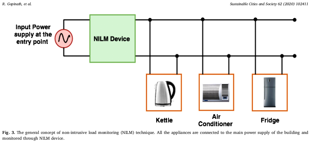
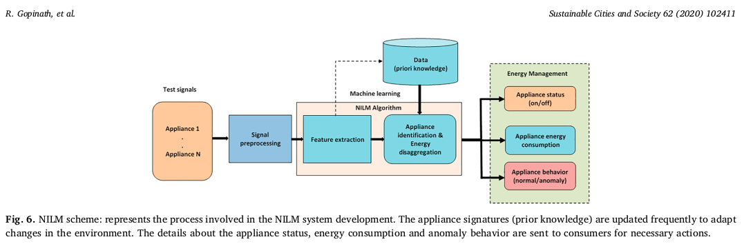
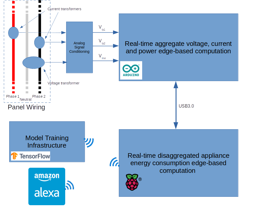
The following first two diagrams illustrate the NILM concept and process steps at a high level. The last diagram shows my prototype system which is based on these concepts and is implemented using Arduino- and Raspberry Pi-based compute.
NILM Algorithm Selection and Models
Algorithm Selection
Energy disaggregation is a highly underdetermined and a single-channel Blind Source Separation (BSS) problem² which makes it difficult to obtain accurate predictions. Let $M$ be the number of household appliances and $i$ be the index referring to the $i$-th appliance. The aggregate power consumption $x$ at a given time $t$ is the sum of the power consumption of all appliances $M$, denoted by $y_i\forall{i=1,...,M}$. Therefore, the total power consumption $x$ at a given time $t$ can expressed by the equation below.
$$ x(t)=\sum_{i=1}^{M} y_i(t) + \epsilon_{\text{noise}}(t) $$
(1)
Where $\epsilon_{noise}$ is a noise term. The goal of this project is to solve the inverse problem and estimate the appliance power consumption $y_i$, given the aggregate power signal $x$, and to do so in a manner suitable for deployment at the edge.
Past approaches have included factorial hidden Markov models (FHMM)¹ and various event-based methods with some success⁶. You can also solve the single-channel BSS problem can by using sequence-to-sequence (seq2seq) learning with neural networks, and it can applied to the NILM problem using transformers, convolutional and recurrent neural networks³. Seq2seq learning involves training a neural network to map between an input time series, such as the aggregate power readings the case of NILM, and a output sequence, such as the estimated energy consumption of a single appliance. A sliding input window is typically used to training the network which generates a corresponding window of the output. This method produces multiple predictions for each appliance in the output so an average of the predictions is used for the final result. Some of the predictions will be more accurate than others, especially those near the midpoint of the input sliding window. The averaging will tend to lower the overall accuracy of the predictions.
Some of the disadvantages of of seq2seq leaning can mitigated by sequence-to-point learning (seq2point) for single-channel BSS⁴. You also use a sliding input signal window in this approach, however the network is trained to predict the output signal only at the midpoint of the window which makes the prediction problem easier on the network, leading to more accurate results.
I selected the seq2point learning approach for my prototype system and my implementation was inspired and guided by work described by Michele D'Incecco, Stefano Squartini and Mingjun Zhong⁵. I developed a variety of seq2point learning models using Tensorflow as shown in the Python module define_models.py but focussed my work on the models transformer and cnn.
Neural Network Models
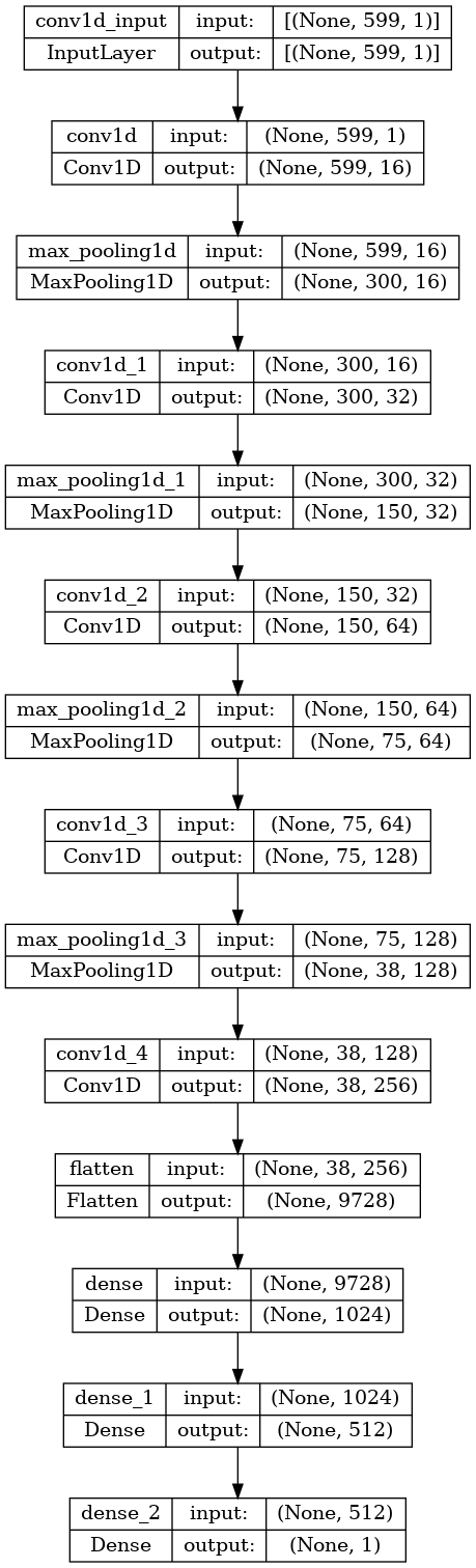
The cnn model is depicted below for an input sequence length of 599 samples. The model generally follows traditional cnn concepts from vision use cases where several convolutional layers are used to extract features from the input power sequence at gradually finer details as the input traverses through the network. These features are the on-off patterns of the appliances as well as their power consumption levels. Max pooling is used to manage the complexity of the model after each convolutional layer. Finally, dense layers are used to output the final single point power consumption estimate for the window which is de-normalized before using in downstream processing. There are about 40 million parameters in this model using the default values.
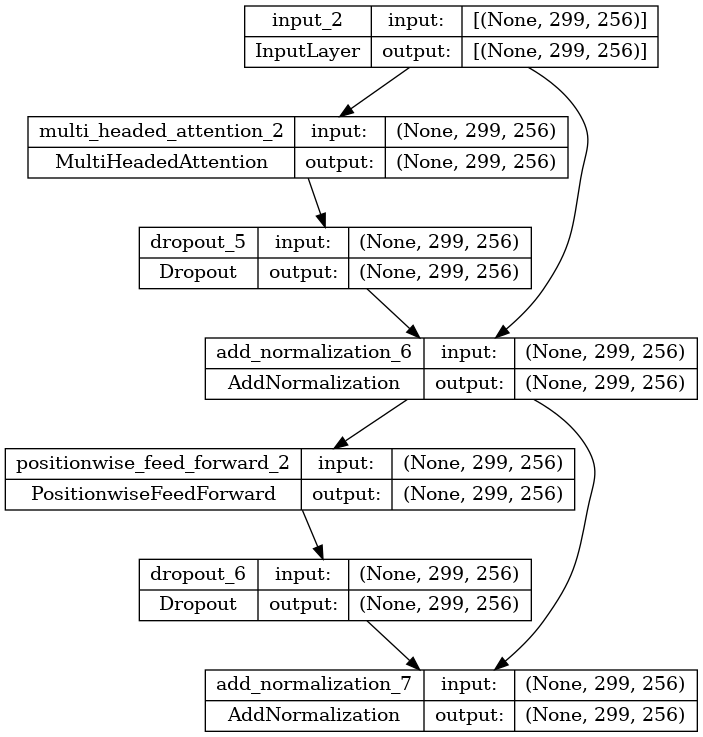
The transformer model is depicted below for an input sequence length of 599 samples where the transformer block is a Bert-style encoder. The input sequence is first passed through a convolutional layer to expand it into a latent space which is analogous to the feature extraction in the cnn model case. These features are pooled and L2 normalized to reduce model complexity and to mitigate the effects of outliers. Next, the sequence features are processed by a Bert-style transformer lineup which includes positional embedding and transformer blocks that applies importance weighting. The output of the encoder is decoded by several layers which are comprised of relative position embedding which applies symmetric weights around the mid-point of the signal, average pooling which reduces the sequence to a single value per feature and then finally dense layers that output the final single point estimated power value for the window which again is de-normalized for downstream processing. There are about six million parameters in this model using the default values.
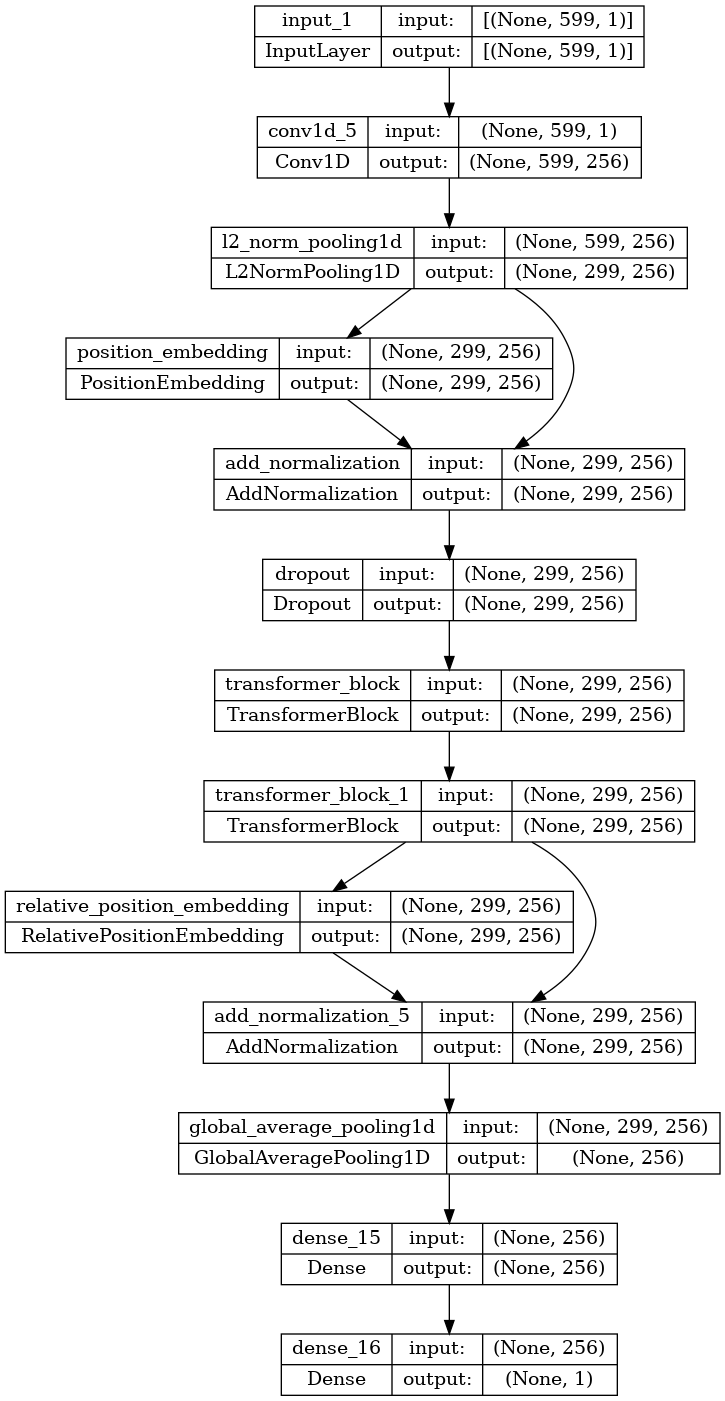
The Bert-style transformer encoder is depicted below.
NILM Datasets
There are a number of large-scale publicly available datasets specifically designed to address the NILM problem which were captured in household buildings from various countries. The table⁷ below shows several of the most widely used.
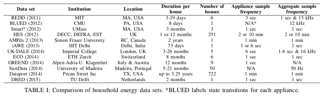
The datasets generally include many 10’s of millions of active power, reactive power, current, and voltage samples but with different sampling frequencies which requires you to pre-process the data before use. Most NILM algorithms utilize only real (aka active or true) power data. Five appliances are usually considered for energy disaggregation research which are kettle, microwave, fridge, dish washer and washing machine. These are the appliances I considered for my prototype and following the work of Michele DIncecco, et al.⁵, I mainly focused on the REFIT⁸ dataset but will eventually include UK-DALE and REDD.
Note that these datasets are typically very imbalanced because the majority of the time an appliance is in the off state.
Model Training and Results
I used TensorFlow to train and test the model. All code associated with this section can be found on the Machine Learning section of the project’s GitHub, NILM⁹. The seq2point learning models for the appliances were trained individually on z-score standardized REFIT data or normalized to $[0, P_m]$, where $P_m$ is the maximum power consumption of an appliance in its active state. Using normalized data tended to give the best model performance so it is used by default.
I used the following metrics to evaluate the model’s performance. You can view the code that calculates these metrics here.
- Mean absolute error ($MAE$), which evaluates the absolute difference between the prediction and the ground truth power at every time point and calculates the mean value, as defined by the equation below.
$$ \mathrm{MAE}=\frac{1}{N}\sum_{i=1}^{N}\lvert \hat{x}_i - x_i\rvert $$
(2)
- Normalized signal aggregate error ($SAE$), which indicates the relative error of the total energy. Denote $r$ as the total energy consumption of the appliance and $\hat{r}$ as the predicted total energy, then SAE is defined per the equation below.
$$ \mathrm{SAE}=\frac{\lvert \hat{r} - r\rvert}{r} $$
(3)
- Energy per Day ($EpD$) which measures the predicted energy used in a day, useful when the household users are interested in the total energy consumed in a period. Denote $D$ as the total number of days and $e=\sum_{t}e_t$ as the appliance energy consumed in a day, then EpD is defined per the equation below.
$$ \mathrm{EpD}=\frac{1}{D}\sum_{n=1}^{D} e_n $$
(4)
- Normalized disaggregation error ($NDE$) which measures the normalized error of the squared difference between the prediction and the ground truth power of the appliances, as defined by the equation below.
$$ \mathrm{NDE}=\frac{\sum_{i,t}\bigl(x_{i,t}-\hat{x}{i,t}\bigr)^2}{\sum{i,t} x_{i,t}^2} $$
(5)
I also used accuracy ($ACC$), F1-score ($F1$) and Matthew’s correlation coefficient ($MCC$) to assess if the model can perform well with the severely imbalanced datasets used to train and test the model. These metrics depend on the on-off status of the device and are computed using the parameters in the common.py module. $ACC$ is equal to the number of correctly predicted time points over the test dataset. $F1$ and $MCC$ are computed according to the equations below where $TP$ stands for true positives, $TN$ stands for true negatives, $FP$ stands for false positives and $FN$ stands for false negatives.
$$ F_1=\frac{TP}{TP+\frac{1}{2}(FP+FN)} $$
(6)
$$ \mathrm{MCC}=\frac{TN\cdot TP - FN\cdot FP}{\sqrt{(TP+FP)(TP+FN)(TN+FP)(TN+FN)}} $$
(7)
$MAE$, $SAE$, $NDE$ and $EpD_e$ (defined as $ 100% \times (EpD_{predicted} - EpD_{ground_truth}) / EpD_{ground_truth}$) reflect the model's ability to correctly predict the appliance energy consumption levels. $F1$ and $MCC$ indicates the model's ability to correctly predict appliance activations using imbalanced classes. $ACC$ is less useful in this application because most of the time the model will correctly predict the appliance is off which dominates the dataset.
A sliding window of 599 samples of the aggregate real power consumption signal is used as inputs to seq2point model and the midpoints of the corresponding windows of the appliances are used as targets. You can see how the samples and targets are generated by an instance of the WindowGenerator Class defined in the window_generator.py module.
You can see the code I used to train the model in train.py which uses the tf.distribute.MirroredStrategy() distributed training strategy. I used the Keras Adam optimizer and to reduce over-fitting, early stopping is used. The training code can be configured to train the seq2point model from scratch, or given a fitted model, prune it or fine tune it with quantization aware training (QAT), both of which can improve inference performance especially on edge hardware.
The key hyper-parameters for training and the optimizer are summarized below.
- Input Window Size: 599 samples
- Global Batch size: 1024 samples.
- From scratch Learning Rate: 1e-04
- QAT and Prune Learning Rate: 1e-05
- Adam Optimizer: beta_1=0.9, beta_2=0.999, epsilon=1e-08.
- Early Stopping Criteria: 6 epochs.
The loss function11 shown in the equation below is used to compute training gradients and to evaluate validation loss on a per-batch basis. It consists of a combination of Mean Squared Error, Binary Cross-Entropy and Mean Absolute Error losses, averaged over distributed model replica batches.
$$ L(x,s) = (\hat{x}-x)^{2} - [\hat{s}\log s + (1-\hat{s})\log(1-s)] + \lambda,|\hat{x}-x| $$
for $\hat{x} \in \mathcal{O}$. (8)
Where $x, \hat{x}\in[0, 1]$ are the ground truth and predicted power usage single point values divided by the maximum power limit per appliance and $s, \hat{s}\in\set{0, 1}$ are the appliance state label and prediction, and $O$ is the set of predictions when either the status label is on or the prediction is incorrect. The hyperparameter $\lambda$ tunes the absolute loss term on an a per-appliance basis.
You can find the training results for each appliance in the models folder. Typical performance metrics for the cnn model are shown in the table below.
| Appliance | $F1\uparrow$ | $MCC\uparrow$ | $ACC\uparrow$ | $MAE$ $(W)$ $\downarrow$ | $SAE\downarrow$ | $NDE\downarrow$ | $EpD_e\thinspace(%)\downarrow$ |
|---|---|---|---|---|---|---|---|
| kettle | 0.7309 | 0.7346 | 0.9960 | 8.788 | 0.2284 | 0.4696 | -22.85 |
| microwave | 0.5671 | 0.5667 | 0.9933 | 7.564 | 0.0460 | 0.8845 | -4.661 |
| fridge | 0.7929 | 0.6942 | 0.8645 | 12.33 | 0.0373 | 0.4111 | 3.733 |
| dishwasher | 0.6069 | 0.6483 | 0.9801 | 5.367 | 0.0347 | 0.3742 | -3.473 |
| washingmachine | 0.8478 | 0.8441 | 0.9893 | 14.75 | 0.2929 | 0.3470 | -29.29 |
Typical performance metrics for the transformer model are shown in the table below.
| Appliance | $F1\uparrow$ | $MCC\uparrow$ | $ACC\uparrow$ | $MAE$ $(W)$ $\downarrow$ | $SAE\downarrow$ | $NDE\downarrow$ | $EpD_e\thinspace(%)\downarrow$ |
|---|---|---|---|---|---|---|---|
| kettle | 0.8177 | 0.8176 | 0.9967 | 7.264 | 0.1348 | 0.3760 | 13.48 |
| microwave | 0.6530 | 0.6506 | 0.9952 | 6.428 | 0.1454 | 0.7496 | -14.54 |
| fridge | 0.8138 | 0.7262 | 0.8799 | 11.02 | 0.0559 | 0.3743 | 5.590 |
| dishwasher | 0.6914 | 0.7119 | 0.9873 | 5.373 | 0.0690 | 0.3906 | -6.904 |
| washingmachine | 0.8435 | 0.8420 | 0.9886 | 14.19 | 0.2440 | 0.2440 | -24.40 |
Average metrics across all appliances for both model architectures are compared in the table below.
| Architecture | $\overline{F1}\uparrow$ | $\overline{MCC}\uparrow$ | $\overline{ACC}\uparrow$ | $\overline{MAE}$ $(W)$ $\downarrow$ | $\overline{SAE}\downarrow$ | $\overline{NDE}\downarrow$ | $\overline{|EpD_e|}\thinspace(%)\downarrow$ |
|---|---|---|---|---|---|---|---|
cnn | 0.7161 | 0.7065 | 0.9643 | 9.852 | 0.1957 | 0.4528 | 19.57 |
transformer | 0.7639 | 0.7497 | 0.9695 | 8.855 | 0.1298 | 0.3781 | 12.98 |
You can see that the cnn and transformer models have similar performance even though the latter has about six times fewer parameters than the former. However, each transformer training step takes about seven times longer than cnn due to the transformer model's use of self-attention which has $O(n^2)$ complexity as compared to the cnn model's $O(n)$, where $n$ is the input sequence length. On the basis on training (and inference) efficiency, you can see that cnn is preferable with little loss in model performance.
You can find a variety of performance metrics in the literature to compare these results against, here are two examples. The middle column in the table5 below shows another cnn-based model's performance. You can see the results of this project compare very favorably.
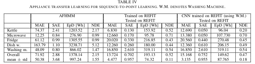
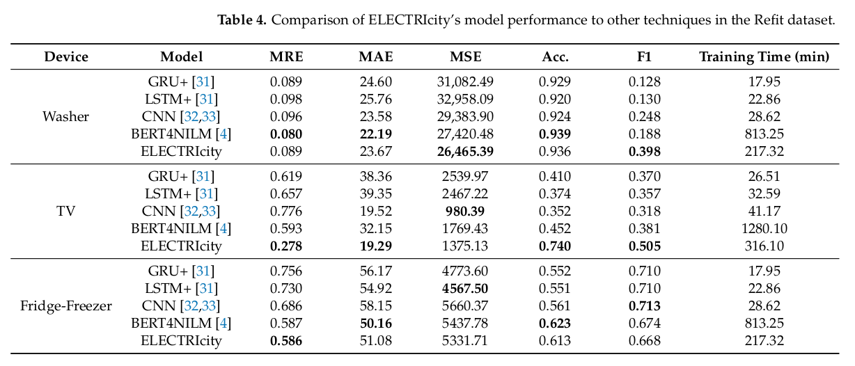
The table12 below shows the results from two transformer-based models (BERT4NILM and ELECTRIcity) and three other architectures. Although the data is incomplete, again this project's transformer-based model results compare favorably.
Model Quantization
I performed Post-training quantization on the cnn and transformer models using the TensorFlow Lite converter API with various quantization modes to improve inference speed on edge hardware, including the Raspberry Pi and the Google Edge TPU, while mitigating the impact on accuracy. You can see the quantization modes I used in the table below.
| Mode | Description |
|---|---|
| convert_only | Convert to tflite but keep all parameters in Float32 (no quantization). |
| w8 | Quantize weights from float32 to int8 and biases to int64. Leave activations in Float32. |
| w8_a8_fallback | Same as w8 but quantize activations from float32 to int8. Fallback to float if an operator does not have an integer implementation. |
| w8_a8 | Same as w8 but quantize activations from float32 to int8. Enforce full int8 quantization for all operators. |
| w8_a16 | Same as w8 but quantize activations to int16. |
The cnn model was quantized using all modes to understand the best tradeoff between latency and accuracy. Only the weights for the transformer model were quantized to int8 using mode w8, the activations needed to be kept in Float32 to maintain acceptable accuracy. See convert_keras_to_tflite.py for the code that does this quantization which also uses TensorFlow Lite's quantization debugger to check how well each layer in the model was quantized. I also profiled the converted models using the TensorFlow Lite Model Benchmark Tool to quantify inference latencies.
The quantized inference results are shown in the tables below, where $L_{x86}$ is the average inference latency on a 3.8 GHz x86 machine using eight tflite interpreter threads and $L_{arm}$ is the average inference latency on the ARM aarch-64-based Raspberry Pi 4 using four threads with both computers using the TensorFlow Lite XNNPACK CPU delegate. $L_{tpu}$ is the average inference latency on the Google Coral Edge TPU. Model inputs and outputs were keep in float32 to maximize inference speed for the x86- and ARM-based machines but were set to int8 for the edge tpu.
CNN Model Results and Discussion
The quantized results for the cnn models are shown in the table below for quantization mode w8.
| Appliance | $F1\uparrow$ | $MCC\uparrow$ | $ACC\uparrow$ | $MAE$ $(W)$ $\downarrow$ | $SAE\downarrow$ | $NDE\downarrow$ | $EpD_e$ ($%$) | $L_{x86}$ (${\mu}s$) | $L_{arm}$ (${\mu}s$) |
|---|---|---|---|---|---|---|---|---|---|
| kettle | 0.7428 | 0.7454 | 0.9966 | 7.371 | 0.2013 | 0.4500 | -20.13 | 743.910 | 3809.41 |
| microwave | 0.6400 | 0.6373 | 0.9933 | 7.971 | 0.1578 | 0.7194 | -15.78 | 736.549 | 3586.55 |
| fridge | 0.6491 | 0.5040 | 0.7935 | 17.78 | 0.0907 | 0.7000 | -8.971 | 731.371 | 3520.54 |
| dishwasher | 0.5143 | 0.5787 | 0.9719 | 5.3955 | 0.0569 | 0.3647 | -5.694 | 742.279 | 3519.52 |
| washingmachine | 0.8838 | 0.8791 | 0.9919 | 15.33 | 0.2930 | 0.3811 | -29.30 | 751.801 | 3515.68 |
The quantized results for the cnn kettle model are shown below for the other quantization modes.
| Mode | $F1\uparrow$ | $MCC\uparrow$ | $ACC\uparrow$ | $MAE$ $(W)$ $\downarrow$ | $SAE\downarrow$ | $NDE\downarrow$ | $EpD_e$ ($%$) | $L_{x86}$ (${\mu}s$) | $L_{arm}$ (${\mu}s$) | $L_{tpu}$ (${\mu}s$) |
|---|---|---|---|---|---|---|---|---|---|---|
| convert_only | 0.7119 | 0.7199 | 0.9964 | 7.812 | 0.2862 | 0.4780 | -28.65 | 309.531 | 12890.10 | NA |
| w8_a8_fallback | 0.6584 | 0.6736 | 0.9959 | 8.677 | 0.3700 | 0.5448 | -36.70 | 186.483 | 3435.56 | NA |
| w8_a8 | 0.6584 | 0.6736 | 0.9960 | 8.768 | 0.3670 | 0.5447 | -36.70 | 185.403 | 3258.19 | 27777.8 |
| w8_a16 | 0.7474 | 0.7479 | 0.9966 | 7.431 | 0.1531 | 0.4516 | -15.31 | 5095.38 | 24065.3 | NA |
The quantized results for the cnn microwave model are shown below for the other quantization modes.
| Mode | $F1\uparrow$ | $MCC\uparrow$ | $ACC\uparrow$ | $MAE$ $(W)$ $\downarrow$ | $SAE\downarrow$ | $NDE\downarrow$ | $EpD_e$ ($%$) | $L_{x86}$ (${\mu}s$) | $L_{arm}$ (${\mu}s$) | $L_{tpu}$ (${\mu}s$) |
|---|---|---|---|---|---|---|---|---|---|---|
| convert_only | 0.6410 | 0.6384 | 0.9933 | 7.976 | 0.1630 | 0.7195 | -18.30 | 302.750 | 13055.3 | NA |
| w8_a8_fallback | 0.6268 | 0.6238 | 0.9931 | 8.006 | 0.1796 | 0.7206 | -17.96 | 187.232 | 3458.30 | NA |
| w8_a8 | 0.6268 | 0.6238 | 0.9931 | 8.005 | 0.1796 | 0.7206 | -17.96 | 183.910 | 3466.65 | 100000 |
| w8_a16 | 0.6391 | 0.6365 | 0.9933 | 7.968 | 0.1590 | 0.7172 | -15.89 | 5100.76 | 24052.0 | NA |
Results for the other appliance models are omitted for brevity but show similar characteristics as a function of quantization mode.
You can see the negative impact of activation quantization but weight quantization, because of regularization effects, has a moderate benefit on some model performance metrics. As expected, the full quantization modes lead to the lowest latencies. Quantizing activations to int16 by the w8_a16 mode results in the highest latencies because only non-optimized reference kernel implementations are presently available in TensorFlow Lite but this scheme leads to the best model metrics given the regularization benefits from weight quantization and better preservation of activation numerics.
You can also see that inference latency of the modes follows w8 ${>}$ convert_only ${>}$ w8_a8 for the x86 machine but convert_only ${>}$ w8 ${>}$ w8_a8 for the aarch64 machine, although the variation is larger for x86. To better understand this, I profiled the converted models using the TFLite Model Benchmark Tool. A summary of the profiling results for the cnn microwave model are shown below which are representative of the other models.
Model Profiling on x86 (slowest to fastest)
You can see that the Fully Connected and Convolution operations are taking the longest to execute in all cases but are much faster in the fully quantized mode of w8_a8.
| w8 node type | count | avg_ms | avg % | cdf % | mem KB | times called |
|---|---|---|---|---|---|---|
| FULLY_CONNECTED | 2 | 0.397 | 56.5527% | 56.5527% | 0 | 2 |
| CONV_2D | 4 | 0.204 | 29.0598% | 85.6125% | 0 | 4 |
| Copy (NC X32) | 2 | 0.051 | 7.26496% | 92.8775% | 0 | 9 |
| Max Pooling (NHWC F32) | 1 | 0.038 | 5.41311% | 98.2906% | 0 | 4 |
| Convolution (NHWC F32) IGEMM | 1 | 0.012 | 1.7094% | 100% | 0 | 1 |
| Fully Connected (NC F32) GEMM | 1 | 0 | 0% | 100% | 0 | 1 |
| EXPAND_DIMS | 9 | 0 | 0% | 100% | 0 | 9 |
| convert_only node type | count | avg_ms | avg % | cdf % | mem KB | times called |
|---|---|---|---|---|---|---|
| Fully Connected (NC F32) GEMM | 3 | 0.151 | 53.3569% | 53.3569% | 0 | 3 |
| Convolution (NHWC F32) IGEMM | 1 | 0.062 | 21.9081% | 75.265% | 0 | 5 |
| Max Pooling (NHWC F32) | 1 | 0.037 | 13.0742% | 88.3392% | 0 | 4 |
| Copy (NC X32) | 1 | 0.033 | 11.6608% | 100% | 0 | 9 |
| EXPAND_DIMS | 9 | 0 | 0% | 100% | 0 | 9 |
| w8_a8 node type | count | avg_ms | avg % | cdf % | mem KB | times called |
|---|---|---|---|---|---|---|
| Convolution (NHWC QC8) IGEMM | 1 | 0.061 | 37.1951% | 37.1951% | 0 | 5 |
| Fully Connected (NC QS8) GEMM | 3 | 0.037 | 22.561% | 59.7561% | 0 | 3 |
| Max Pooling (NHWC S8) | 1 | 0.034 | 20.7317% | 80.4878% | 0 | 4 |
| Copy (NC X8) | 1 | 0.032 | 19.5122% | 100% | 0 | 9 |
| EXPAND_DIMS | 9 | 0 | 0% | 100% | 0 | 9 |
| Convert (NC QS8 F32) | 1 | 0 | 0% | 100% | 0 | 1 |
| Convert (NC F32 QS8) | 1 | 0 | 0% | 100% | 0 | 1 |
Model Profiling on aarch64 (slowest to fastest)
You can see the copy and Max Pooling operations in particular are relatively slower on x86 than on aarch64 which is probably due to memory bandwidth and micro-architecture differences.
| convert_only node type | count | avg_ms | avg % | cdf % | mem KB | times called |
|---|---|---|---|---|---|---|
| Copy (NC X32) | 1 | 34.835 | 30.9136% | 30.9136% | 0 | 9 |
| Convolution (NHWC F32) IGEMM | 1 | 32.414 | 28.7651% | 59.6787% | 0 | 5 |
| Max Pooling (NHWC F32) | 1 | 23.008 | 20.418% | 80.0967% | 0 | 4 |
| Fully Connected (NC F32) GEMM | 3 | 22.425 | 19.9006% | 99.9973% | 0 | 3 |
| EXPAND_DIMS | 9 | 0.003 | 0.00266229% | 100% | 0 | 9 |
| w8 node type | count | avg_ms | avg % | cdf % | mem KB | times called |
|---|---|---|---|---|---|---|
| Max Pooling (NHWC F32) | 1 | 42.281 | 46.9085% | 46.9085% | 0 | 4 |
| CONV_2D | 4 | 17.461 | 19.3721% | 66.2806% | 0 | 4 |
| Copy (NC X32) | 2 | 16.877 | 18.7241% | 85.0047% | 0 | 9 |
| Convolution (NHWC F32) IGEMM | 1 | 10.658 | 11.8245% | 96.8292% | 0 | 1 |
| FULLY_CONNECTED | 2 | 2.847 | 3.1586% | 99.9878% | 0 | 2 |
| Fully Connected (NC F32) GEMM | 1 | 0.007 | 0.00776613% | 99.9956% | 0 | 1 |
| EXPAND_DIMS | 9 | 0.004 | 0.00443779% | 100% | 0 | 9 |
| w8_a8 node type | count | avg_ms | avg % | cdf % | mem KB | times called |
|---|---|---|---|---|---|---|
| Copy (NC X8) | 1 | 34.686 | 30.9647% | 30.9647% | 0 | 9 |
| Convolution (NHWC QC8) IGEMM | 1 | 33.259 | 29.6908% | 60.6554% | 0 | 5 |
| Max Pooling (NHWC S8) | 1 | 23.922 | 21.3555% | 82.0109% | 0 | 4 |
| Fully Connected (NC QS8) GEMM | 3 | 20.146 | 17.9846% | 99.9955% | 0 | 3 |
| EXPAND_DIMS | 9 | 0.002 | 0.00178543% | 99.9973% | 0 | 9 |
| Convert (NC F32 QS8) | 1 | 0.002 | 0.00178543% | 99.9991% | 0 | 1 |
| Convert (NC QS8 F32) | 1 | 0.001 | 0.000892714% | 100% | 0 | 1 |
Quantization Efficacy
The RMSE / scale is close to $1 / sqrt(12)$ (~ 0.289) when quantized distribution is similar to the original float distribution, indicating a well-quantized model. The larger the value is, it's more likely for the layer not being quantized well. The tables below show the RMSE / Scale metric for the cnn kettle and cnn washingmachine models and the Suspected? column indicates a layer that significantly exceeds 0.289. Other models are omitted for brevity but show similar results. These layers can remain in float to generate a selectively quantized model that increases accuracy at the expense of inference performance but doing so for the cnn models did not materially improve accuracy. See Inspecting Quantization Errors with Quantization Debugger.
Layer quantization efficacy metrics for the cnn kettle model using mode w8_a8 are shown below.
| layer | op_name | range | rmse/scale | Suspected? |
|---|---|---|---|---|
| 0 | EXPAND_DIMS | 23.929975 | 2.75E-01 | |
| 1 | CONV_2D | 5.518012 | 2.22E-01 | |
| 2 | RESHAPE | 5.518012 | 2.38E-06 | |
| 3 | EXPAND_DIMS | 5.518012 | 2.38E-06 | |
| 4 | MAX_POOL_2D | 5.518012 | 2.42E-06 | |
| 5 | RESHAPE | 5.518012 | 2.42E-06 | |
| 6 | EXPAND_DIMS | 5.518012 | 2.42E-06 | |
| 7 | CONV_2D | 3.494575 | 1.79E-01 | |
| 8 | RESHAPE | 3.494575 | 1.44E-06 | |
| 9 | EXPAND_DIMS | 3.494575 | 1.44E-06 | |
| 10 | MAX_POOL_2D | 3.494575 | 1.49E-06 | |
| 11 | RESHAPE | 3.494575 | 1.49E-06 | |
| 12 | EXPAND_DIMS | 3.494575 | 1.49E-06 | |
| 13 | CONV_2D | 5.910911 | 1.22E-01 | |
| 14 | RESHAPE | 5.910911 | 1.09E-06 | |
| 15 | EXPAND_DIMS | 5.910911 | 1.09E-06 | |
| 16 | MAX_POOL_2D | 5.910911 | 1.18E-06 | |
| 17 | RESHAPE | 5.910911 | 1.18E-06 | |
| 18 | EXPAND_DIMS | 5.910911 | 1.18E-06 | |
| 19 | CONV_2D | 10.82671 | 1.00E-01 | |
| 20 | RESHAPE | 10.82671 | 1.00E-06 | |
| 21 | EXPAND_DIMS | 10.82671 | 1.00E-06 | |
| 22 | MAX_POOL_2D | 10.82671 | 1.08E-06 | |
| 23 | RESHAPE | 10.82671 | 1.08E-06 | |
| 24 | EXPAND_DIMS | 10.82671 | 1.08E-06 | |
| 25 | CONV_2D | 2.987664 | 5.77E-02 | |
| 26 | RESHAPE | 2.987664 | 3.82E-07 | |
| 27 | FULLY_CONNECTED | 1.725032 | 1.20E+00 | Yes |
| 28 | FULLY_CONNECTED | 1.512342 | 6.19E-01 | |
| 29 | FULLY_CONNECTED | 0.990833 | 2.03E+00 | Yes |
Layer quantization efficacy metrics for the cnn washingmachine model using mode w8_a8 are shown below.
| layer | op_name | range | rmse/scale | Suspected? |
|---|---|---|---|---|
| 0 | EXPAND_DIMS | 30.954547 | 3.00E-01 | |
| 1 | CONV_2D | 12.620701 | 1.81E-01 | |
| 2 | RESHAPE | 12.620701 | 1.56E-06 | |
| 3 | EXPAND_DIMS | 12.620701 | 1.56E-06 | |
| 4 | MAX_POOL_2D | 12.620701 | 1.67E-06 | |
| 5 | RESHAPE | 12.620701 | 1.67E-06 | |
| 6 | EXPAND_DIMS | 12.620701 | 1.67E-06 | |
| 7 | CONV_2D | 15.030776 | 1.94E-01 | |
| 8 | RESHAPE | 15.030776 | 1.94E-07 | |
| 9 | EXPAND_DIMS | 15.030776 | 1.94E-07 | |
| 10 | MAX_POOL_2D | 15.030776 | 2.36E-07 | |
| 11 | RESHAPE | 15.030776 | 2.36E-07 | |
| 12 | EXPAND_DIMS | 15.030776 | 2.36E-07 | |
| 13 | CONV_2D | 10.132236 | 1.68E-01 | |
| 14 | RESHAPE | 10.132236 | 1.83E-06 | |
| 15 | EXPAND_DIMS | 10.132236 | 1.83E-06 | |
| 16 | MAX_POOL_2D | 10.132236 | 2.06E-06 | |
| 17 | RESHAPE | 10.132236 | 2.06E-06 | |
| 18 | EXPAND_DIMS | 10.132236 | 2.06E-06 | |
| 19 | CONV_2D | 9.038437 | 1.45E-01 | |
| 20 | RESHAPE | 9.038437 | 1.90E-06 | |
| 21 | EXPAND_DIMS | 9.038437 | 1.90E-06 | |
| 22 | MAX_POOL_2D | 9.038437 | 2.20E-06 | |
| 23 | RESHAPE | 9.038437 | 2.20E-06 | |
| 24 | EXPAND_DIMS | 9.038437 | 2.20E-06 | |
| 25 | CONV_2D | 5.151932 | 9.58E-02 | |
| 26 | RESHAPE | 5.151932 | 1.08E-06 | |
| 27 | FULLY_CONNECTED | 7.269378 | 1.13E-01 | |
| 28 | FULLY_CONNECTED | 3.79172 | 1.75E-01 | |
| 29 | FULLY_CONNECTED | 1.102378 | 9.51E-01 | Yes |
Model Memory Footprint
I used the TFLite Model Benchmark Tool to get the approximate RAM consumption of the TFLite cnn microwave model at runtime which is shown in the table below for each quantization mode as well as the TFLite model disk space. The other cnn models show similar characteristics. The findings for the x86 architecture were identical to the arm architecture. Note that the Keras model consumes about 42.49 (MB) on disk. You can see that there is about a four times reduction in disk storage space due to the float32 to int8 weight conversions. Interestingly, RAM runtime usage varies considerably due to the TFLite algorithms that that optimize intermediate tensors usage. These are pre-allocated to reduce inference latency at the cost of memory space. See Optimizing TensorFlow Lite Runtime Memory.
| Quant Mode | Disk (MB) | RAM (MB) |
|---|---|---|
| convert_only | 42.485044 | 84.957 |
| w8 | 10.642040 | 12.7109 |
| w8_a8 | 10.648016 | 23.3633 |
| w8_a16 | 10.660984 | 10.1836 |
Transformer Model Results and Discussion
Note that even though the XNNPACK delagate was enabled during transformer model inference evaluation nothing was actually accelerated because the transformer model contains dynamic tensors. The following warning is shown when using the TFLite interpreter for inference:
Attempting to use a delegate that only supports static-sized tensors with a graph that has dynamic-sized tensors (tensor#94 is a dynamic-sized tensor).
This means that all operators are unsupported by XNNPACK and will fall back to the default CPU kernel implementations. A future effort will involve refactoring the transformer model use only static-size tensors. Note that a tensor could be marked dynamic at TFLite runtime when there is a control-flow operation (e.g., if, while etc.) prepared. In other words, even when the model graph itself doesn't have any tensors of dynamic shapes statically, at runtime a model could have dynamic tensors. The current transformer model uses if control-flow operations.
The quantized results for the transformer model are shown in the table below for quantization mode w8.
| Appliance | $F1\uparrow$ | $MCC\uparrow$ | $ACC\uparrow$ | $MAE$ $(W)$ $\downarrow$ | $SAE\downarrow$ | $NDE\downarrow$ | $EpD_e$ ($%$) | $L_{x86}$ (${\mu}s$) | $L_{arm}$ (${\mu}s$) |
|---|---|---|---|---|---|---|---|---|---|
| kettle | 0.8460 | 0.8483 | 0.9977 | 5.117 | 0.1761 | 0.2760 | -17.61 | 20520 | 61939 |
| microwave | 0.7375 | 0.7355 | 0.9952 | 6.969 | 0.3435 | 0.6049 | -34.35 | 20905 | 60823 |
| fridge | 0.7437 | 0.6261 | 0.8381 | 14.52 | 0.0838 | 0.5518 | -8.560 | 20986 | 61862 |
| dishwasher | 0.6671 | 0.6905 | 0.9860 | 6.214 | 0.1117 | 0.4521 | -11.17 | 20983 | 63432 |
| washingmachine | 0.8910 | 0.8872 | 0.9926 | 15.08 | 0.3796 | 0.3442 | -37.96 | 21426 | 60901 |
The quantized results for the transformer kettle and microwave models are shown in the table below for quantization mode convert_only.
| Appliance | $F1\uparrow$ | $MCC\uparrow$ | $ACC\uparrow$ | $MAE$ $(W)$ $\downarrow$ | $SAE\downarrow$ | $NDE\downarrow$ | $EpD_e$ ($%$) | $L_{x86}$ (${\mu}s$) | $L_{arm}$ (${\mu}s$) |
|---|---|---|---|---|---|---|---|---|---|
| kettle | 0.8460 | 0.8483 | 0.9977 | 5.117 | 0.1761 | 0.2760 | -17.61 | 7100 | 69746 |
| microwave | 0.6719 | 0.6736 | 0.9948 | 7.054 | 0.3930 | 0.6518 | -39.30 | 7050 | 68667 |
Model Profiling on x86 (slowest to fastest)
| w8 node type | count | avg_ms | avg % | cdf % | mem KB | times called |
|---|---|---|---|---|---|---|
| FULLY_CONNECTED | 14 | 16.243 | 79.5485% | 79.5485% | 0 | 14 |
| ADD | 41 | 0.667 | 3.26657% | 82.815% | 0 | 41 |
| MUL | 42 | 0.661 | 3.23718% | 86.0522% | 0 | 42 |
| BATCH_MATMUL | 4 | 0.582 | 2.85029% | 88.9025% | 0 | 4 |
| TRANSPOSE | 20 | 0.551 | 2.69847% | 91.601% | 0 | 20 |
| RESHAPE | 48 | 0.384 | 1.8806% | 93.4816% | 0 | 48 |
| POW | 2 | 0.371 | 1.81694% | 95.2985% | 0 | 2 |
| SOFTMAX | 2 | 0.202 | 0.989275% | 96.2878% | 0 | 2 |
| MEAN | 13 | 0.177 | 0.86684% | 97.1546% | 0 | 13 |
| CONV_2D | 1 | 0.152 | 0.744405% | 97.899% | 0 | 1 |
| SQUARED_DIFFERENCE | 6 | 0.119 | 0.582791% | 98.4818% | 0 | 6 |
| TANH | 2 | 0.11 | 0.538714% | 99.0205% | 0 | 2 |
| AVERAGE_POOL_2D | 1 | 0.086 | 0.421176% | 99.4417% | 0 | 1 |
| FILL | 14 | 0.059 | 0.288947% | 99.7306% | 0 | 14 |
| SQUARE | 1 | 0.036 | 0.176306% | 99.9069% | 0 | 1 |
| SQRT | 1 | 0.019 | 0.0930506% | 100% | 0 | 1 |
| SUB | 6 | 0 | 0% | 100% | 0 | 6 |
| STRIDED_SLICE | 14 | 0 | 0% | 100% | 0 | 14 |
| SHAPE | 24 | 0 | 0% | 100% | 0 | 24 |
| RSQRT | 6 | 0 | 0% | 100% | 0 | 6 |
| REDUCE_PROD | 16 | 0 | 0% | 100% | 0 | 16 |
| PACK | 22 | 0 | 0% | 100% | 0 | 22 |
| GATHER | 16 | 0 | 0% | 100% | 0 | 16 |
| EXPAND_DIMS | 2 | 0 | 0% | 100% | 0 | 2 |
| CONCATENATION | 8 | 0 | 0% | 100% | 0 | 8 |
| convert_only node type | count | avg_ms | avg % | cdf % | mem KB | times called |
|---|---|---|---|---|---|---|
| FULLY_CONNECTED | 14 | 2.211 | 31.0447% | 31.0447% | 0 | 14 |
| ADD | 41 | 1.344 | 18.8711% | 49.9158% | 0 | 41 |
| MUL | 42 | 0.693 | 9.73041% | 59.6462% | 0 | 42 |
| RESHAPE | 48 | 0.619 | 8.69138% | 68.3375% | 0 | 48 |
| BATCH_MATMUL | 4 | 0.529 | 7.42769% | 75.7652% | 0 | 4 |
| TRANSPOSE | 20 | 0.4 | 5.6164% | 81.3816% | 0 | 20 |
| POW | 2 | 0.394 | 5.53215% | 86.9138% | 0 | 2 |
| MEAN | 13 | 0.216 | 3.03286% | 89.9466% | 0 | 13 |
| SOFTMAX | 2 | 0.155 | 2.17636% | 92.123% | 0 | 2 |
| SQUARED_DIFFERENCE | 6 | 0.128 | 1.79725% | 93.9202% | 0 | 6 |
| TANH | 2 | 0.119 | 1.67088% | 95.5911% | 0 | 2 |
| AVERAGE_POOL_2D | 1 | 0.102 | 1.43218% | 97.0233% | 0 | 1 |
| FILL | 14 | 0.099 | 1.39006% | 98.4134% | 0 | 14 |
| CONV_2D | 1 | 0.051 | 0.716091% | 99.1294% | 0 | 1 |
| SQUARE | 1 | 0.037 | 0.519517% | 99.649% | 0 | 1 |
| SQRT | 1 | 0.025 | 0.351025% | 100% | 0 | 1 |
| SUB | 6 | 0 | 0% | 100% | 0 | 6 |
| STRIDED_SLICE | 14 | 0 | 0% | 100% | 0 | 14 |
| SHAPE | 24 | 0 | 0% | 100% | 0 | 24 |
| RSQRT | 6 | 0 | 0% | 100% | 0 | 6 |
| REDUCE_PROD | 16 | 0 | 0% | 100% | 0 | 16 |
| PACK | 22 | 0 | 0% | 100% | 0 | 22 |
| GATHER | 16 | 0 | 0% | 100% | 0 | 16 |
| EXPAND_DIMS | 2 | 0 | 0% | 100% | 0 | 2 |
| CONCATENATION | 8 | 0 | 0% | 100% | 0 | 8 |
Model Profiling on aarch64 (slowest to fastest)
| convert_only node type | count | avg_ms | avg % | cdf % | mem KB | times called |
|---|---|---|---|---|---|---|
| FULLY_CONNECTED | 14 | 30.777 | 44.8716% | 44.8716% | 0 | 14 |
| MUL | 42 | 8.571 | 12.4962% | 57.3678% | 0 | 42 |
| ADD | 41 | 7.425 | 10.8254% | 68.1931% | 0 | 41 |
| POW | 2 | 5.308 | 7.73885% | 75.932% | 0 | 2 |
| BATCH_MATMUL | 4 | 3.82 | 5.56941% | 81.5014% | 0 | 4 |
| TRANSPOSE | 20 | 3.352 | 4.88708% | 86.3885% | 0 | 20 |
| RESHAPE | 48 | 2.927 | 4.26745% | 90.6559% | 0 | 48 |
| TANH | 2 | 2.02 | 2.94508% | 93.601% | 0 | 2 |
| SOFTMAX | 2 | 1.182 | 1.72331% | 95.3243% | 0 | 2 |
| MEAN | 13 | 0.927 | 1.35153% | 96.6758% | 0 | 13 |
| SQUARED_DIFFERENCE | 6 | 0.761 | 1.10951% | 97.7854% | 0 | 6 |
| AVERAGE_POOL_2D | 1 | 0.517 | 0.753765% | 98.5391% | 0 | 1 |
| SQUARE | 1 | 0.326 | 0.475295% | 99.0144% | 0 | 1 |
| CONV_2D | 1 | 0.281 | 0.409687% | 99.4241% | 0 | 1 |
| SQRT | 1 | 0.148 | 0.215778% | 99.6399% | 0 | 1 |
| PACK | 22 | 0.105 | 0.153086% | 99.793% | 0 | 22 |
| FILL | 14 | 0.077 | 0.112263% | 99.9052% | 0 | 14 |
| SUB | 6 | 0.022 | 0.0320751% | 99.9373% | 0 | 6 |
| RSQRT | 6 | 0.022 | 0.0320751% | 99.9694% | 0 | 6 |
| STRIDED_SLICE | 14 | 0.012 | 0.0174955% | 99.9869% | 0 | 14 |
| SHAPE | 24 | 0.005 | 0.0072898% | 99.9942% | 0 | 24 |
| EXPAND_DIMS | 2 | 0.003 | 0.00437388% | 99.9985% | 0 | 2 |
| CONCATENATION | 8 | 0.001 | 0.00145796% | 100% | 0 | 8 |
| REDUCE_PROD | 16 | 0 | 0% | 100% | 0 | 16 |
| GATHER | 16 | 0 | 0% | 100% | 0 | 16 |
| w8 node type | count | avg_ms | avg % | cdf % | mem KB | times called |
|---|---|---|---|---|---|---|
| FULLY_CONNECTED | 14 | 22.759 | 38.6283% | 38.6283% | 0 | 14 |
| MUL | 42 | 7.718 | 13.0996% | 51.7278% | 0 | 42 |
| ADD | 41 | 6.952 | 11.7994% | 63.5273% | 0 | 41 |
| POW | 2 | 5.074 | 8.61197% | 72.1392% | 0 | 2 |
| BATCH_MATMUL | 4 | 3.773 | 6.40382% | 78.5431% | 0 | 4 |
| TRANSPOSE | 20 | 2.982 | 5.06127% | 83.6043% | 0 | 20 |
| RESHAPE | 48 | 2.902 | 4.92549% | 88.5298% | 0 | 48 |
| TANH | 2 | 1.95 | 3.30968% | 91.8395% | 0 | 2 |
| SOFTMAX | 2 | 1.222 | 2.07407% | 93.9136% | 0 | 2 |
| MEAN | 13 | 0.91 | 1.54452% | 95.4581% | 0 | 13 |
| SQUARED_DIFFERENCE | 6 | 0.79 | 1.34085% | 96.7989% | 0 | 6 |
| CONV_2D | 1 | 0.659 | 1.1185% | 97.9174% | 0 | 1 |
| AVERAGE_POOL_2D | 1 | 0.48 | 0.814692% | 98.7321% | 0 | 1 |
| SQUARE | 1 | 0.359 | 0.609321% | 99.3414% | 0 | 1 |
| SQRT | 1 | 0.126 | 0.213857% | 99.5553% | 0 | 1 |
| PACK | 22 | 0.107 | 0.181608% | 99.7369% | 0 | 22 |
| FILL | 14 | 0.082 | 0.139176% | 99.8761% | 0 | 14 |
| SUB | 6 | 0.025 | 0.0424319% | 99.9185% | 0 | 6 |
| RSQRT | 6 | 0.023 | 0.0390373% | 99.9576% | 0 | 6 |
| STRIDED_SLICE | 14 | 0.013 | 0.0220646% | 99.9796% | 0 | 14 |
| EXPAND_DIMS | 2 | 0.005 | 0.00848637% | 99.9881% | 0 | 2 |
| SHAPE | 24 | 0.004 | 0.0067891% | 99.9949% | 0 | 24 |
| GATHER | 16 | 0.002 | 0.00339455% | 99.9983% | 0 | 16 |
| CONCATENATION | 8 | 0.001 | 0.00169727% | 100% | 0 | 8 |
| REDUCE_PROD | 16 | 0 | 0% | 100% | 0 | 16 |
Quantization Efficacy
Layer quantization efficacy metrics for the transformer kettle model using mode w8_a8 are shown in the table below, although as noted above quantizing the transformer model's activations results in very poor model performance. You can see the RSQRT operator in particular does not quantize well, these operators are used in the Gaussian error linear activation functions which helps explain the poor performance of the model. The other transformer appliance models show similar efficacy metrics.
| layer | op_name | range | rmse/scale | Suspect? |
|---|---|---|---|---|
| 0 | EXPAND_DIMS | 23.929975 | 0.2751951 | |
| 1 | CONV_2D | 6.793423 | 0.2952648 | |
| 2 | RESHAPE | 12.080546 | 0.1608947 | |
| 3 | EXPAND_DIMS | 12.080546 | 0 | |
| 4 | AVERAGE_POOL_2D | 12.080546 | 0 | |
| 5 | ADD | 11.598116 | 0.03801457 | |
| 6 | RESHAPE | 3.405601 | 0.0580239 | |
| 7 | FILL | 1 | 0 | |
| 8 | MUL | 0.489979 | 0.2888043 | |
| 9 | ADD | 3.72709 | 0.2890081 | |
| 10 | FILL | 1 | 0 | |
| 11 | FILL | 2E-06 | 0 | |
| 12 | RESHAPE | 3.72709 | 0 | |
| 13 | TRANSPOSE | 3.72709 | 0 | |
| 14 | MEAN | 1.371433 | 0.3178885 | |
| 15 | SQUARED_DIFFERENCE | 4.45292 | 0.2296307 | |
| 16 | MEAN | 0.547054 | 0.2962779 | |
| 17 | ADD | 0.548054 | 0.4589049 | |
| 18 | RSQRT | 15.745848 | 41.5733 | Yes |
| 19 | MUL | 15.745848 | 0 | |
| 20 | MUL | 9.606549 | 0.3037147 | |
| 21 | MUL | 2.384117 | 0.2467738 | |
| 22 | SUB | 2.384117 | 1.428423E-06 | |
| 23 | ADD | 8.792654 | 0.3326802 | |
| 24 | TRANSPOSE | 8.792654 | 0 | |
| 25 | RESHAPE | 8.792654 | 0 | |
| 26 | MUL | 8.606096 | 0.2844383 | |
| 27 | ADD | 8.682471 | 0.2893911 | |
| 28 | RESHAPE | 8.682471 | 0 | |
| 29 | FULLY_CONNECTED | 13.589397 | 0.337322 | |
| 30 | RESHAPE | 13.589397 | 0 | |
| 31 | ADD | 13.66659 | 0.2940356 | |
| 32 | RESHAPE | 13.66659 | 0 | |
| 33 | TRANSPOSE | 13.66659 | 0 | |
| 34 | FULLY_CONNECTED | 16.061866 | 0.3192651 | |
| 35 | RESHAPE | 16.061866 | 0 | |
| 36 | ADD | 16.14824 | 0.2843503 | |
| 37 | RESHAPE | 16.14824 | 0 | |
| 38 | TRANSPOSE | 16.14824 | 0 | |
| 39 | BATCH_MATMUL | 791.061 | 0.2887679 | |
| 40 | MUL | 69.920572 | 1.274111E-06 | |
| 41 | SOFTMAX | 0.996094 | 0.1901133 | |
| 42 | FULLY_CONNECTED | 15.370091 | 0.3185204 | |
| 43 | RESHAPE | 15.370091 | 0 | |
| 44 | ADD | 15.420575 | 0.273666 | |
| 45 | RESHAPE | 15.420575 | 0 | |
| 46 | TRANSPOSE | 15.420575 | 0 | |
| 47 | BATCH_MATMUL | 13.788238 | 0.2886845 | |
| 48 | TRANSPOSE | 13.788238 | 0 | |
| 49 | RESHAPE | 13.788238 | 0 | |
| 50 | RESHAPE | 13.788238 | 0 | |
| 51 | FULLY_CONNECTED | 13.103168 | 0.3028338 | |
| 52 | RESHAPE | 13.103168 | 0 | |
| 53 | ADD | 13.229318 | 0.2886953 | |
| 54 | ADD | 15.80188 | 0.288787 | |
| 55 | FILL | 1 | 0 | |
| 56 | FILL | 2E-06 | 0 | |
| 57 | RESHAPE | 15.80188 | 0 | |
| 58 | TRANSPOSE | 15.80188 | 0 | |
| 59 | MEAN | 0.345499 | 0.4923606 | |
| 60 | SQUARED_DIFFERENCE | 63.224075 | 0.2779759 | |
| 61 | MEAN | 4.931316 | 0.3027504 | |
| 62 | ADD | 4.932316 | 0.0311987 | |
| 63 | RSQRT | 1.195838 | 0.304619 | |
| 64 | MUL | 1.195838 | 0 | |
| 65 | MUL | 10.555507 | 0.2823485 | |
| 66 | MUL | 0.219467 | 0.4081438 | |
| 67 | SUB | 0.219467 | 2.18255E-06 | |
| 68 | ADD | 10.513915 | 0.2897937 | |
| 69 | TRANSPOSE | 10.513915 | 0 | |
| 70 | RESHAPE | 10.513915 | 0 | |
| 71 | MUL | 11.164726 | 0.2816773 | |
| 72 | ADD | 11.191346 | 0.2954707 | |
| 73 | RESHAPE | 11.191346 | 0 | |
| 74 | FULLY_CONNECTED | 20.655138 | 0.3090305 | |
| 75 | RESHAPE | 20.655138 | 0 | |
| 76 | ADD | 20.650391 | 0.3390533 | |
| 77 | MUL | 99.871166 | 0.2299994 | |
| 78 | ADD | 120.521553 | 0.2948375 | |
| 79 | MUL | 96.162275 | 9.767714E-07 | |
| 80 | TANH | 1.992188 | 0.2440195 | |
| 81 | ADD | 2 | 0.2198295 | |
| 82 | MUL | 10.325196 | 0 | |
| 83 | MUL | 9.776829 | 0.4144 | |
| 84 | RESHAPE | 9.776829 | 0 | |
| 85 | FULLY_CONNECTED | 83.573343 | 0.2907445 | |
| 86 | RESHAPE | 83.573343 | 0 | |
| 87 | ADD | 83.595579 | 0.08025211 | |
| 88 | ADD | 85.804338 | 0.2887958 | |
| 89 | FILL | 1 | 0 | |
| 90 | FILL | 2E-06 | 0 | |
| 91 | RESHAPE | 85.804338 | 0 | |
| 92 | TRANSPOSE | 85.804338 | 0 | |
| 93 | MEAN | 0.671132 | 0.3675501 | |
| 94 | SQUARED_DIFFERENCE | 2199.59073 | 0.2545643 | |
| 95 | MEAN | 175.261857 | 0.2906021 | |
| 96 | ADD | 175.262859 | 0.001332498 | |
| 97 | RSQRT | 0.985917 | inf | Yes |
| 98 | MUL | 0.985917 | 0 | |
| 99 | MUL | 10.02912 | 0.2857049 | |
| 100 | MUL | 0.143655 | 0.2965899 | |
| 101 | SUB | 0.143655 | 1.620293E-06 | |
| 102 | ADD | 10.016886 | 0.273117 | |
| 103 | TRANSPOSE | 10.016886 | 0 | |
| 104 | RESHAPE | 10.016886 | 0 | |
| 105 | MUL | 10.061665 | 0.2678465 | |
| 106 | ADD | 10.07655 | 0.2902205 | |
| 107 | RESHAPE | 10.07655 | 0 | |
| 108 | FULLY_CONNECTED | 24.452702 | 0.305032 | |
| 109 | RESHAPE | 24.452702 | 0 | |
| 110 | ADD | 24.471723 | 0.2637686 | |
| 111 | RESHAPE | 24.471723 | 0 | |
| 112 | TRANSPOSE | 24.471723 | 0 | |
| 113 | FULLY_CONNECTED | 24.602528 | 0.3068753 | |
| 114 | RESHAPE | 24.602528 | 0 | |
| 115 | ADD | 24.524895 | 0.2782782 | |
| 116 | RESHAPE | 24.524895 | 0 | |
| 117 | TRANSPOSE | 24.524895 | 0 | |
| 118 | BATCH_MATMUL | 2375.91354 | 0.2896734 | |
| 119 | MUL | 210.003057 | 2.292973E-06 | |
| 120 | SOFTMAX | 0.996094 | 0.05637038 | |
| 121 | FULLY_CONNECTED | 20.075173 | 0.3076454 | |
| 122 | RESHAPE | 20.075173 | 0 | |
| 123 | ADD | 20.075706 | 0.263613 | |
| 124 | RESHAPE | 20.075706 | 0 | |
| 125 | TRANSPOSE | 20.075706 | 0 | |
| 126 | BATCH_MATMUL | 19.701535 | 0.2828629 | |
| 127 | TRANSPOSE | 19.701535 | 0 | |
| 128 | RESHAPE | 19.701535 | 0 | |
| 129 | RESHAPE | 19.701535 | 0 | |
| 130 | FULLY_CONNECTED | 93.741001 | 0.2932989 | |
| 131 | RESHAPE | 93.741001 | 0 | |
| 132 | ADD | 93.754804 | 0.07540143 | |
| 133 | ADD | 98.071743 | 0.2887844 | |
| 134 | FILL | 1 | 0 | |
| 135 | FILL | 2E-06 | 0 | |
| 136 | RESHAPE | 98.071743 | 0 | |
| 137 | TRANSPOSE | 98.071743 | 0 | |
| 138 | MEAN | 0.733764 | 0.2978907 | |
| 139 | SQUARED_DIFFERENCE | 2799.43284 | 0.2259659 | |
| 140 | MEAN | 47.061099 | 0.3333294 | |
| 141 | ADD | 47.062096 | 0.00378661 | |
| 142 | RSQRT | 0.887359 | 0.932645 | Yes |
| 143 | MUL | 0.887359 | 0 | |
| 144 | MUL | 17.251803 | 0.2807441 | |
| 145 | MUL | 0.272383 | 0.2891514 | |
| 146 | SUB | 0.272383 | 1.761181E-06 | |
| 147 | ADD | 17.311272 | 0.3122337 | |
| 148 | TRANSPOSE | 17.311272 | 0 | |
| 149 | RESHAPE | 17.311272 | 0 | |
| 150 | MUL | 17.347451 | 0.2828182 | |
| 151 | ADD | 17.347451 | 0.2636831 | |
| 152 | RESHAPE | 17.347451 | 0 | |
| 153 | FULLY_CONNECTED | 18.324211 | 0.3175219 | |
| 154 | RESHAPE | 18.324211 | 0 | |
| 155 | ADD | 18.343422 | 0.3259408 | |
| 156 | MUL | 69.135855 | 0.2440944 | |
| 157 | ADD | 87.47928 | 0.2834869 | |
| 158 | MUL | 69.798363 | 4.807578E-07 | |
| 159 | TANH | 1.992188 | 0.3179474 | |
| 160 | ADD | 2 | 0.2156563 | |
| 161 | MUL | 9.171711 | 0 | |
| 162 | MUL | 9.578754 | 0.2946312 | |
| 163 | RESHAPE | 9.578754 | 0 | |
| 164 | FULLY_CONNECTED | 364.467573 | 0.2889795 | |
| 165 | RESHAPE | 364.467573 | 0 | |
| 166 | ADD | 364.406858 | 0.01272385 | |
| 167 | ADD | 371.900848 | 0.2615761 | |
| 168 | FILL | 1 | 0 | |
| 169 | FILL | 2E-06 | 0 | |
| 170 | RESHAPE | 371.900848 | 0 | |
| 171 | TRANSPOSE | 371.900848 | 0 | |
| 172 | MEAN | 5.672659 | 0.3749806 | |
| 173 | SQUARED_DIFFERENCE | 37128.26265 | 0.1978192 | |
| 174 | MEAN | 2799.73527 | 0.2974154 | |
| 175 | ADD | 2799.73629 | 7.520764E-05 | |
| 176 | RSQRT | 0.991143 | inf | Yes |
| 177 | MUL | 0.991143 | 0 | |
| 178 | MUL | 14.455902 | 2.44185 | Yes |
| 179 | MUL | 0.352157 | 14.605 | Yes |
| 180 | SUB | 0.352157 | 2.75764E-06 | |
| 181 | ADD | 14.478933 | 0.3361114 | |
| 182 | TRANSPOSE | 14.478933 | 0 | |
| 183 | RESHAPE | 14.478933 | 0 | |
| 184 | MUL | 16.685117 | 0.2978353 | |
| 185 | ADD | 16.703711 | 0.2075399 | |
| 186 | FILL | 1 | 0 | |
| 187 | MUL | 0.424291 | 0.2876463 | |
| 188 | ADD | 16.933183 | 0.2892929 | |
| 189 | FILL | 1 | 0 | |
| 190 | FILL | 2E-06 | 0 | |
| 191 | RESHAPE | 16.933183 | 0 | |
| 192 | TRANSPOSE | 16.933183 | 0 | |
| 193 | MEAN | 0.062335 | 48.13572 | Yes |
| 194 | SQUARED_DIFFERENCE | 85.610105 | 0.2268296 | |
| 195 | MEAN | 1.226184 | 381.2859 | Yes |
| 196 | ADD | 1.227184 | 0.01558558 | |
| 197 | RSQRT | 1.094414 | 0.3163588 | |
| 198 | MUL | 1.094414 | 0 | |
| 199 | MUL | 15.961633 | 0.2128369 | |
| 200 | MUL | 0.06705 | 0.2904581 | |
| 201 | SUB | 0.06705 | 2.78254E-06 | |
| 202 | ADD | 15.949823 | 0.2522852 | |
| 203 | TRANSPOSE | 15.949823 | 0 | |
| 204 | RESHAPE | 15.949823 | 0 | |
| 205 | MUL | 13.885122 | 0.2597474 | |
| 206 | ADD | 13.780075 | 0.3595855 | |
| 207 | MEAN | 4.198399 | 0.3065109 | |
| 208 | FULLY_CONNECTED | 2.434557 | 0.3960356 | |
| 209 | FULLY_CONNECTED | 0.733557 | 9.714286 | Yes |
Model Memory Footprint
Identical to the cnn case, I used the TFLite Model Benchmark Tool to get the approximate RAM consumption of the TFLite microwave model at runtime which is shown in the table below for each relevant quantization mode as well as the TFLite model disk space. The other transformer models show similar characteristics. Note that the Keras model consumes about 6.02 (MB) on disk. You can see that there is about a three times reduction in model size due to the weights being quantized from float32 to int8 which is less than the four times reduction seen in the cnn case likely because there are fewer layers with weights. You can also see that the x86 TFLite runtime is more memory efficient than its aarch64 counterpart for this model.
| Quant Mode | Disk (MB) | aarch64 RAM (MB) | x86 RAM (MB) |
|---|---|---|---|
| convert_only | 6.217276 | 20.8242 | 16.8438 |
| w8 | 2.088312 | 16.4258 | 13.3789 |
NILM Prototype System Components
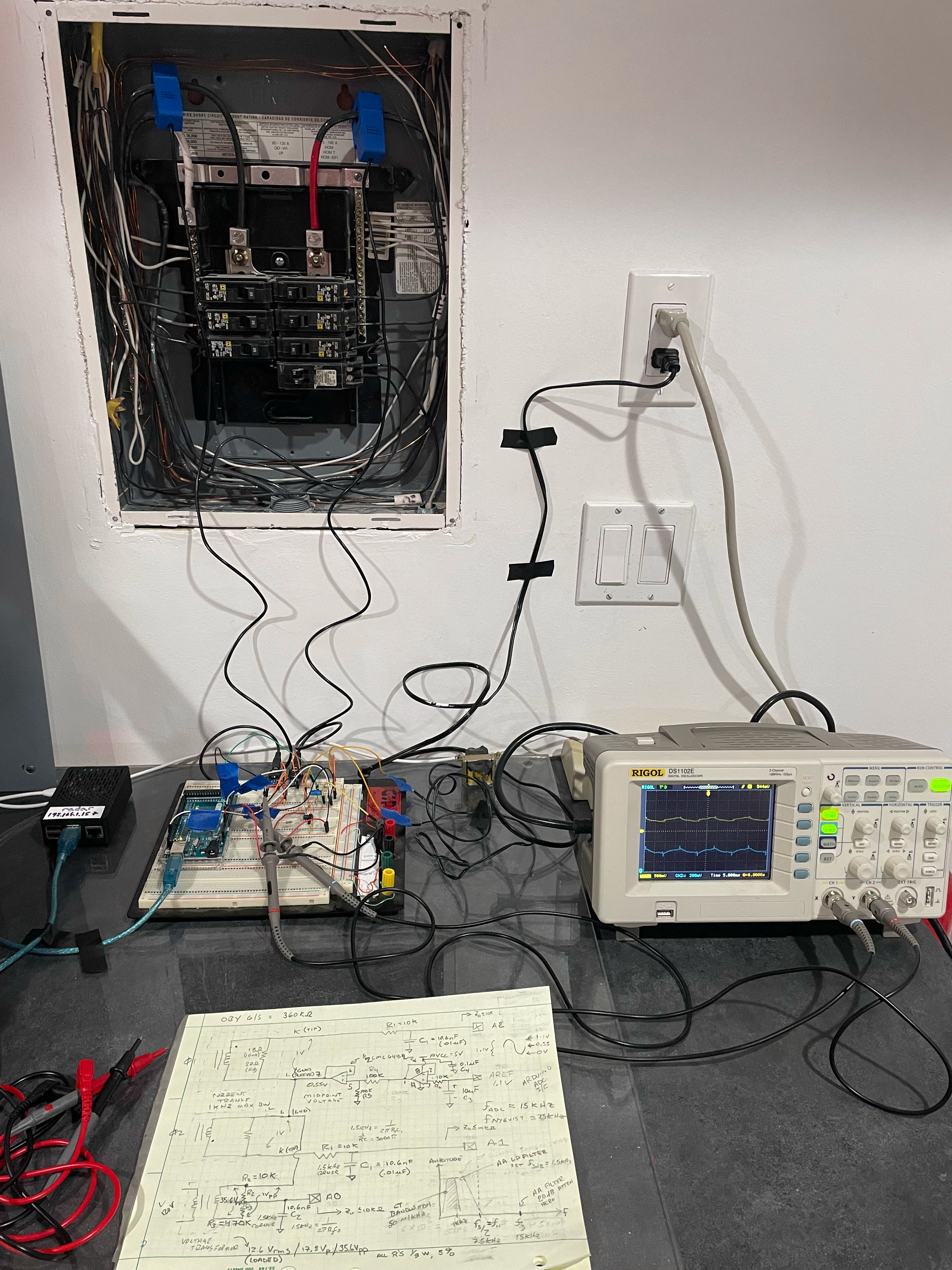
I built a NILM prototype at my home to test the energy disaggregation algorithms in real-world conditions and to understand where they can be improved. The prototype is comprised of the following main subsystems. You can see a photograph of the prototype in the Appendix.
Analog Signal Conditioning
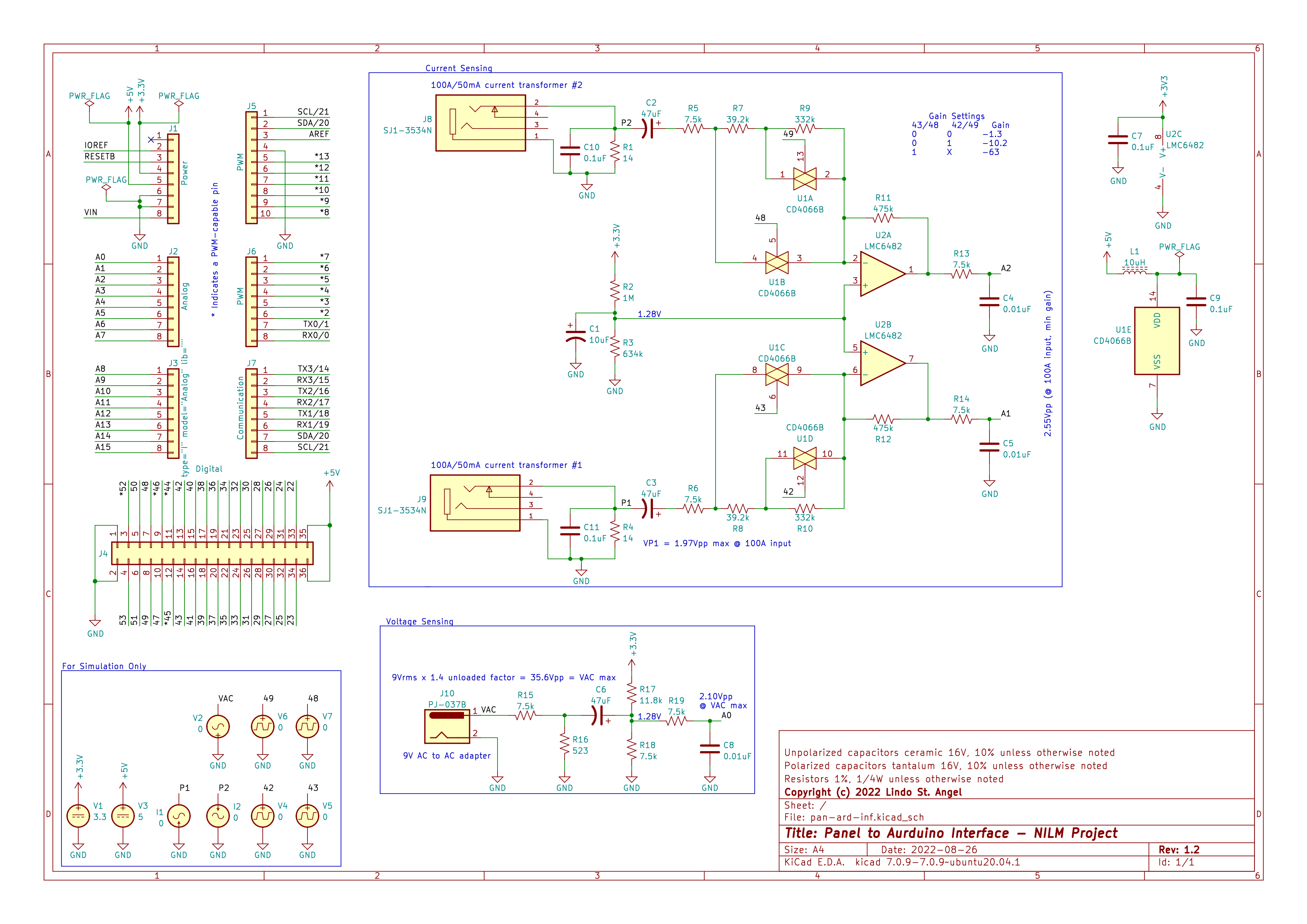
I used two clip-on current transformers in one of the home’s sub-panels to sense the current flowing through each of split voltage phases and a voltage transformer plugged into an outlet near the circuit breaker panel that provides the voltage of one of the phases. These signals are level-shifted, amplified and low-passed filtered by this subsystem before being passed on to the analog-to-digital converters inside an Arduino MEGA 2560 that performs aggregate metrics computation. You can see a schematic for the Analog Signal Conditioning Subsystem in the Appendix and find more details in the Panel to Arduino section.
Aggregate Metrics Computation
I used an Arduino MEGA 2560 to host the signal processing algorithms that takes the voltage signals from the Analog Signal Conditioning Subsystem and generates aggregate RMS voltage, RMS current, Real Power and Apparent Power metrics in real-time. Presently, only Real Power is used in downstream processing. I leveraged emonLibCM10 for these signal processing algorithms. emonLibCM runs continuously in the background and digitizes the analog input channels of the Arduino, calculates these metrics and then informs the Arduino sketch that the measurements are available and should be read and processed by downstream processing. The sketch is configured to update the metrics every eight seconds and can be found in ard.ino
Disaggregated Energy Consumption Computation
The actual energy disaggregation computations are hosted on a Raspberry Pi 4 which is connected over USB to the Arduino to fetch the aggregate metrics. The computations are comprised of running the tflite appliance inference models, trained and quantized per the steps described above, with pre- and post-processing steps. See the infer.py module for the code that performs these computations. The inference models output predicted energy for each appliance from 599-sample sized windows of the aggregate real power input signal. These predictions and aggregate mains power are stored in a local CSV file and made available for downstream reporting and analysis.
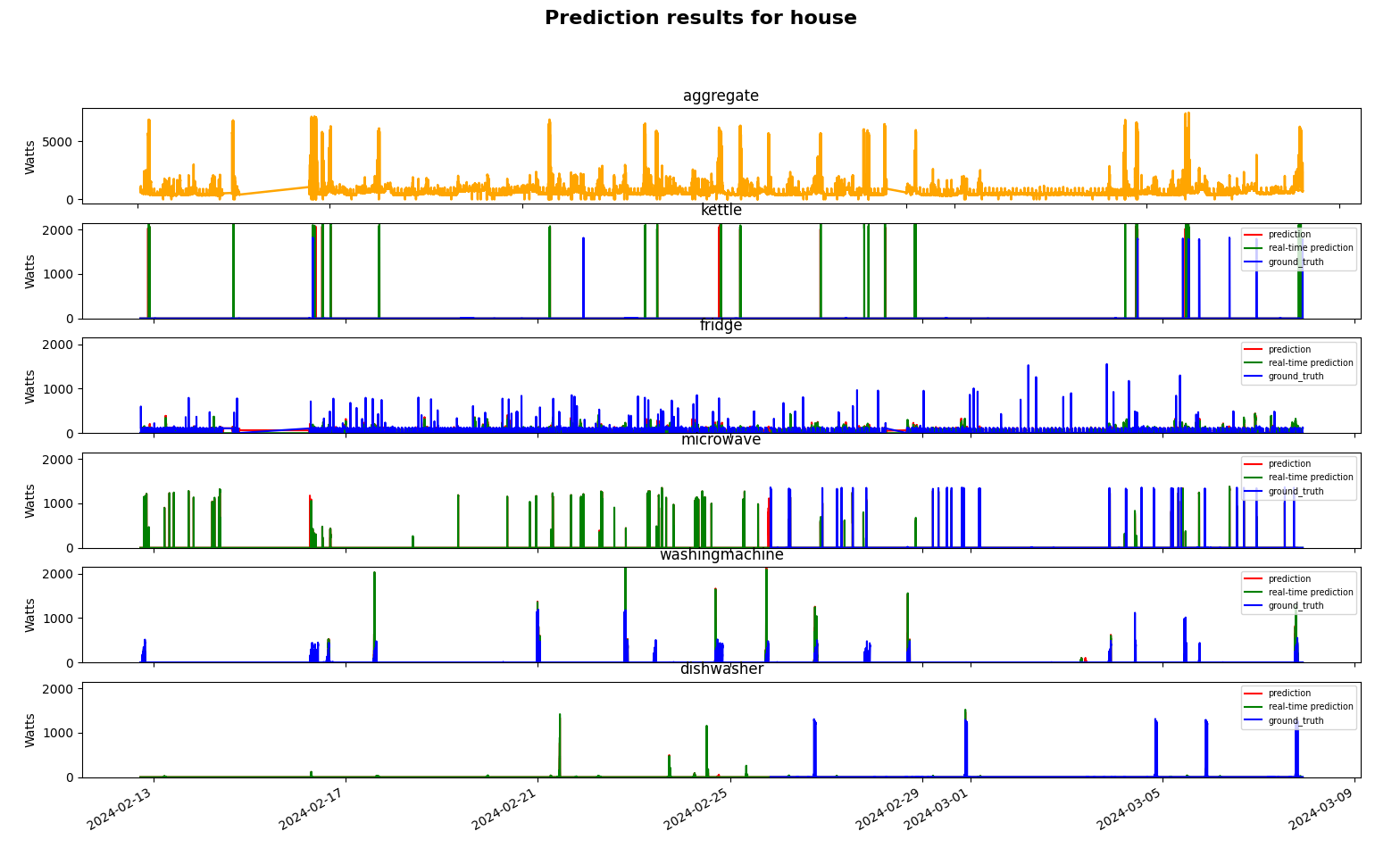
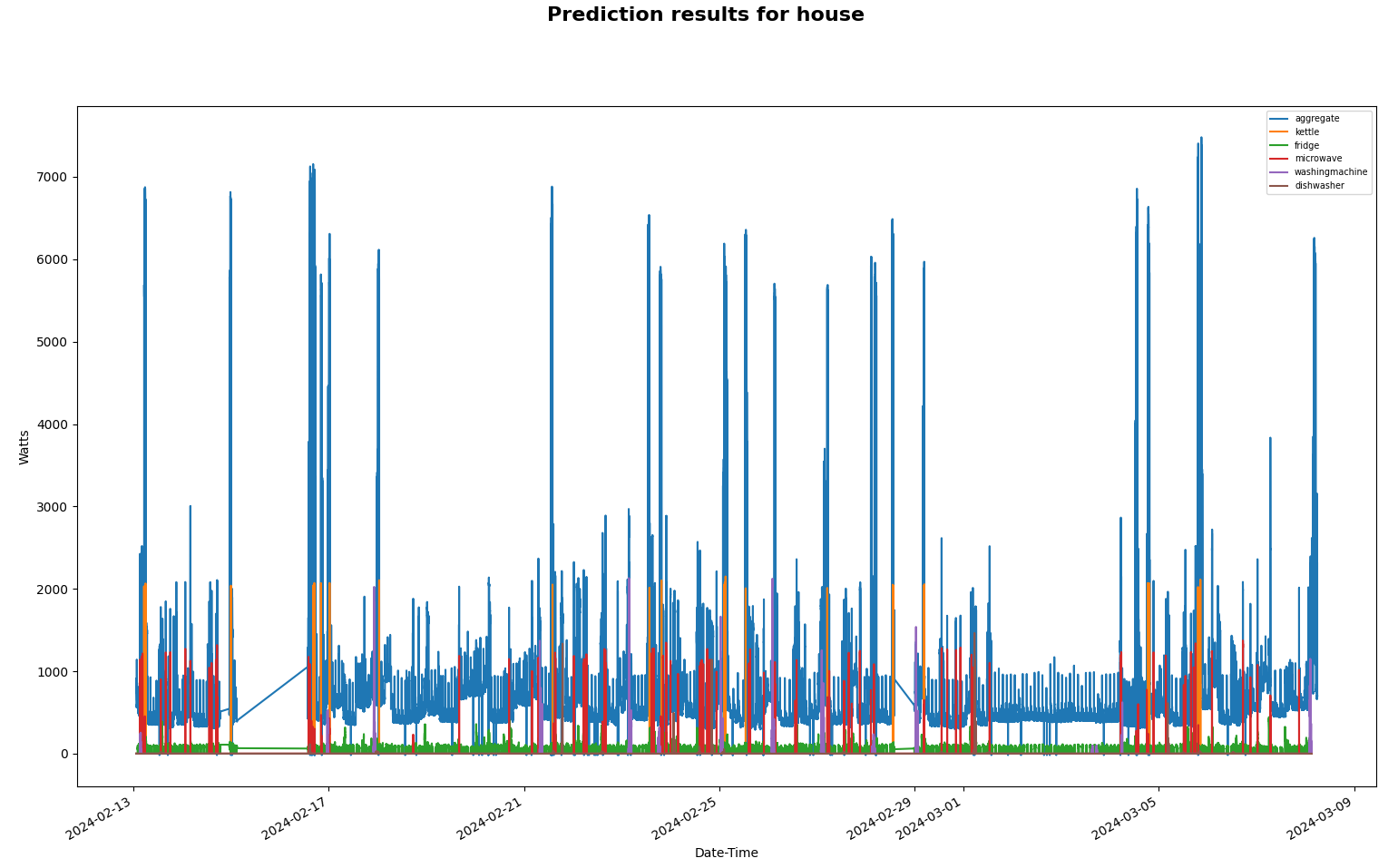
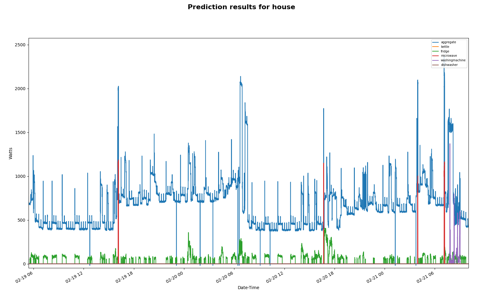
Typical disaggregated energy prediction results from my home are shown in the plots and tables below using tflite models trained on another machine from the dataset as described above and quantized using mode 'w8'. Two sets of results are shown, the first is with no fine-tuning and second, with fine-tuning using local data via the program fine_tune.
In the plots below, the horizontal axis is datetime. The vertical axis is energy consumption in Watts. The first plot shows the aggregate mains power with each appliance in separate sub-plots. Ground truth power was obtained by logging appliance power data in real-time at the outlet. The second plat shows aggregate mains power and appliance power plotted together and the last plot is a zoomed-in area of the second plot. These plots and the metrics that follow are generated by the program predict.
NILM metrics were computed for the Float32 predictions on aggregate mains data that was captured in real-time and for the quantized model real-time predictions, both vs ground truth.
The Float32 model trained on the default dataset predictions vs ground truth are shown in the table below.
| Appliance | $F1\uparrow$ | $MCC\uparrow$ | $ACC\uparrow$ | $MAE$ $(W)$ $\downarrow$ | $SAE\downarrow$ | $NDE\downarrow$ | $EpD_e$ ($%$) |
|---|---|---|---|---|---|---|---|
| kettle | 0.0 | NaN | 0.9918 | 1.659 | INF | 0.9999 | INF |
| microwave | 0.5319 | 0.5406 | 0.9961 | 4.261 | 0.0302 | 0.8198 | -3.018 |
| fridge | 0.6875 | 0.4672 | 0.7414 | 36.59 | 0.2458 | 0.7494 | -24.56 |
| dishwasher | 0.2372 | 0.2165 | 0.9596 | 12.74 | 0.9586 | 0.9615 | -95.62 |
| washingmachine | 0.6661 | 0.6696 | 0.9749 | 7.596 | 0.2213 | 1.407 | -23.97 |
The corresponding quantized model real-time predictions vs ground truth are shown in the table below.
| Appliance | $F1\uparrow$ | $MCC\uparrow$ | $ACC\uparrow$ | $MAE$ $(W)$ $\downarrow$ | $SAE\downarrow$ | $NDE\downarrow$ | $EpD_e$ ($%$) |
|---|---|---|---|---|---|---|---|
| kettle | 0.0 | NaN | 0.9986 | 2.873 | INF | 1.594 | INF |
| microwave | 0.5258 | 0.5353 | 0.9961 | 4.237 | 0.0188 | 0.8208 | -1.880 |
| fridge | 0.6257 | 0.4002 | 0.7125 | 39.52 | 0.3668 | 0.8189 | -36.65 |
| dishwasher | 0.2571 | 0.2354 | 0.9469 | 14.70 | 0.9557 | 0.9558 | -95.57 |
| washingmachine | 0.6760 | 0.6827 | 0.9758 | 7.560 | 0.2401 | 1.393 | -24.01 |
You can see that model performance is comparable between the Float32 and real-time quantized results but overall they are poor with microwave being the exception. This indicates that the models can benefit from fine tuning with the ground truth data.
The Float32 model fine-tuned with local data predictions vs ground truth are shown in the table below.
| Appliance | $F1\uparrow$ | $MCC\uparrow$ | $ACC\uparrow$ | $MAE$ $(W)$ $\downarrow$ | $SAE\downarrow$ | $NDE\downarrow$ | $EpD_e$ ($%$) |
|---|---|---|---|---|---|---|---|
| kettle | 0.6205 | 0.6672 | 0.9958 | 7.808 | 0.5716 | 0.5555 | -57.16 |
| microwave | 0.4989 | 0.5129 | 0.9912 | 10.508 | 0.6543 | 0.6795 | -65.43 |
| fridge | 0.8286 | 0.6665 | 0.8312 | 24.705 | 0.2502 | 0.3717 | -25.02 |
| dishwasher | 0.7607 | 0.7491 | 0.9544 | 21.911 | 0.4602 | 0.3957 | -46.02 |
| washingmachine | 0.9155 | 0.9138 | 0.9905 | 3.288 | 0.1156 | 0.3535 | -11.56 |
The corresponding quantized model real-time predictions vs ground truth are shown in the table below.
| Appliance | $F1\uparrow$ | $MCC\uparrow$ | $ACC\uparrow$ | $MAE$ $(W)$ $\downarrow$ | $SAE\downarrow$ | $NDE\downarrow$ | $EpD_e$ ($%$) |
|---|---|---|---|---|---|---|---|
| kettle | 0.5845 | 0.6345 | 0.9955 | 8.199 | 0.5918 | 0.5954 | -59.18 |
| microwave | 0.5221 | 0.5196 | 0.9904 | 10.722 | 0.5781 | 0.6574 | -57.81 |
| fridge | 0.8351 | 0.6758 | 0.8367 | 26.137 | 0.2477 | 0.3603 | -24.27 |
| dishwasher | 0.6188 | 0.6230 | 0.9083 | 23.506 | 0.2313 | 0.3414 | -23.13 |
| washingmachine | 0.7103 | 0.7257 | 0.9585 | 3.910 | 0.2454 | 0.3409 | 24.54 |
You can see that fine-tuning the model with local data greatly improves its performance.
Amazon Alexa
I plan to use Amazon Alexa as the user interface to the appliance energy data, however this work is not yet started.
Conclusion
By using large publicly available datasets to train seq2point learning models it is very feasible to perform energy disaggregation that is fairly accurate without fine-tuning the models with local data. These models are modest in size and with little loss in accuracy can be quantized to run efficiently on commodity edge hardware such as the Raspberry Pi 4. More work needs to be done to further improve the accuracy of the models and to test with more appliance types. This project demonstrates that a key component of a sustainable and scalable power grid is within reach of the mass consumer market.
References
- Sustainable Cities and Society 62 (2020) 102411 | Energy management using non-intrusive load monitoring techniques — State- of-the-art and future research directions by R. Gopinath, Mukesh Kumar, C. Prakash Chandra Joshua and Kota Srinivas.
- Wikipedia | Signal Separation.
- arXiv:1507.06594 | Neural NILM: Deep Neural Networks Applied to Energy Disaggregation by Jack Kelly and William Knottenbelt.
- arXiv:1612.09106 | Sequence-to-point learning with neural networks for non-intrusive load monitoring by Chaoyun Zhang, Mingjun Zhong, Zongzuo Wang, Nigel Goddard and Charles Sutton.
- arXiv:1902.08835 | Transfer Learning for Non-Intrusive Load Monitoring by Michele D'Incecco, Stefano Squartini and Mingjun Zhong.
- Artificial Intelligence Techniques for a Scalable Energy Transition pp 109–131 | A Review on Non-intrusive Load Monitoring Approaches Based on Machine Learning by Hajer Salem, Moamar Sayed-Mouchaweh and Moncef Tagina.
- 1st International Symposium on Signal Processing Applications in Smart Buildings at 3rd IEEE Global Conference on Signal & Information Processing | Dataport and NILMTK: A Building Data Set Designed for Non-intrusive Load Monitoring by Oliver Parson, Grant Fisher, April Hersey, Nipun Batra, Jack Kelly, Amarjeet Singh, William Knottenbelt and Alex Rogers.
- Proceedings of the 8th International Conference on Energy Efficiency in Domestic Appliances and Lighting | A data management platform for personalised real-time energy feedback by David Murray and Jing Liao and Lina Stankovic and Vladimir Stankovic and Richard Hauxwell-Baldwin and Charlie Wilson and Michael Coleman and Tom Kane and Steven Firth. The REFIT dataset used in this project is is licensed under the Creative Commons Attribution 4.0 International Public License.
- GitHub | NILM by Lindo St. Angel
- GitHub | EmonLibCM by Trystan Lea, Glyn Hudson, Brian Orpin and Ivan Kravets.
- BERT4NILM: A Bidirectional Transformer Model for Non-Intrusive Load Monitoring by Zhenrui Yue, et. al.
- ELECTRIcity: An Efficient Transformer for Non-Intrusive Load Monitoring by Stavros Sykiotis, Maria Kaselimi ,Anastasios Doulamis and Nikolaos Doulamis.
Please also see this project's companion Medium article Energy Management Using Real-Time Non-Intrusive Load Monitoring.
Appendix
Photograph of Prototype
A photograph of an early version of my prototype system is shown below.
Analog Signal Conditioning Schematic
The schematic for the Analog Signal Conditioning circuitry is shown below.
Contributors

104 commits
Similar repos


Languages
Python
96.8%
C++
2.9%
Energy Management Using Real-Time Non-Intrusive Load Monitoring
Python
104
104 commits
updated Sep 8, 2025
See what people are saying (1)
README
Energy Management Using Real-Time Non-Intrusive Load Monitoring
Introduction
The goal of non-intrusive load monitoring (NILM) is to recover the energy consumption of individual appliances from the aggregate mains signal, which is a measure of the total electricity consumption of a building or house. NILM is also known as energy disaggregation and both terms will be used interchangeably throughout.
R. Gopinath, et al., nicely summarizes the rational behind NILM in the paper Energy management using non-intrusive load monitoring techniques — State- of-the-art and future research directions¹:
In recent years, the development of smart sustainable cities has become the primary focus among urban planners and policy makers to make responsible use of resources, conserve the environment and improve the well-being of the society. Energy management is an integral part of the smart sustainable cities development programme which involves conscious and efficient use of available energy resources towards attaining sustainability and self-reliance on energy systems. Building sector is one of the key sectors that utilize more energy. Therefore, efforts are being made to monitor and manage energy consumption effectively in residential and commercial buildings. In recent years, non-intrusive load monitoring (NILM) technique has become a popular and emerging approach to monitor events (on/off) and energy consumption of appliances/electrical utilities in buildings using single energy meter. The information about the energy consumption at the appliance level would help consumers to understand their appliance usage behavior and take necessary steps for reducing energy consumption.
By using deep learning models trained on publicly available datasets it is now feasible to enable NILM in very cost effective ways by leveraging commodity hardware and open source software. Deploying the trained models at the edge of the power grid, i.e. the building level, results in additional cost savings since it obviates the need for always connected internet cloud services which can be expensive at scale and running the algorithms in real-time provides for low latency operation.
This Project will show you how NILM works by taking you through the steps I used to implement a prototype system at my house.
Architecture
The following first two diagrams illustrate the NILM concept and process steps at a high level. The last diagram shows my prototype system which is based on these concepts and is implemented using Arduino- and Raspberry Pi-based compute.
NILM Algorithm Selection and Models
Algorithm Selection
Energy disaggregation is a highly underdetermined and a single-channel Blind Source Separation (BSS) problem² which makes it difficult to obtain accurate predictions. Let $M$ be the number of household appliances and $i$ be the index referring to the $i$-th appliance. The aggregate power consumption $x$ at a given time $t$ is the sum of the power consumption of all appliances $M$, denoted by $y_i\forall{i=1,...,M}$. Therefore, the total power consumption $x$ at a given time $t$ can expressed by the equation below.
$$ x(t)=\sum_{i=1}^{M} y_i(t) + \epsilon_{\text{noise}}(t) $$
(1)
Where $\epsilon_{noise}$ is a noise term. The goal of this project is to solve the inverse problem and estimate the appliance power consumption $y_i$, given the aggregate power signal $x$, and to do so in a manner suitable for deployment at the edge.
Past approaches have included factorial hidden Markov models (FHMM)¹ and various event-based methods with some success⁶. You can also solve the single-channel BSS problem can by using sequence-to-sequence (seq2seq) learning with neural networks, and it can applied to the NILM problem using transformers, convolutional and recurrent neural networks³. Seq2seq learning involves training a neural network to map between an input time series, such as the aggregate power readings the case of NILM, and a output sequence, such as the estimated energy consumption of a single appliance. A sliding input window is typically used to training the network which generates a corresponding window of the output. This method produces multiple predictions for each appliance in the output so an average of the predictions is used for the final result. Some of the predictions will be more accurate than others, especially those near the midpoint of the input sliding window. The averaging will tend to lower the overall accuracy of the predictions.
Some of the disadvantages of of seq2seq leaning can mitigated by sequence-to-point learning (seq2point) for single-channel BSS⁴. You also use a sliding input signal window in this approach, however the network is trained to predict the output signal only at the midpoint of the window which makes the prediction problem easier on the network, leading to more accurate results.
I selected the seq2point learning approach for my prototype system and my implementation was inspired and guided by work described by Michele D'Incecco, Stefano Squartini and Mingjun Zhong⁵. I developed a variety of seq2point learning models using Tensorflow as shown in the Python module define_models.py but focussed my work on the models transformer and cnn.
Neural Network Models
The cnn model is depicted below for an input sequence length of 599 samples. The model generally follows traditional cnn concepts from vision use cases where several convolutional layers are used to extract features from the input power sequence at gradually finer details as the input traverses through the network. These features are the on-off patterns of the appliances as well as their power consumption levels. Max pooling is used to manage the complexity of the model after each convolutional layer. Finally, dense layers are used to output the final single point power consumption estimate for the window which is de-normalized before using in downstream processing. There are about 40 million parameters in this model using the default values.
The transformer model is depicted below for an input sequence length of 599 samples where the transformer block is a Bert-style encoder. The input sequence is first passed through a convolutional layer to expand it into a latent space which is analogous to the feature extraction in the cnn model case. These features are pooled and L2 normalized to reduce model complexity and to mitigate the effects of outliers. Next, the sequence features are processed by a Bert-style transformer lineup which includes positional embedding and transformer blocks that applies importance weighting. The output of the encoder is decoded by several layers which are comprised of relative position embedding which applies symmetric weights around the mid-point of the signal, average pooling which reduces the sequence to a single value per feature and then finally dense layers that output the final single point estimated power value for the window which again is de-normalized for downstream processing. There are about six million parameters in this model using the default values.
The Bert-style transformer encoder is depicted below.
NILM Datasets
There are a number of large-scale publicly available datasets specifically designed to address the NILM problem which were captured in household buildings from various countries. The table⁷ below shows several of the most widely used.
The datasets generally include many 10’s of millions of active power, reactive power, current, and voltage samples but with different sampling frequencies which requires you to pre-process the data before use. Most NILM algorithms utilize only real (aka active or true) power data. Five appliances are usually considered for energy disaggregation research which are kettle, microwave, fridge, dish washer and washing machine. These are the appliances I considered for my prototype and following the work of Michele DIncecco, et al.⁵, I mainly focused on the REFIT⁸ dataset but will eventually include UK-DALE and REDD.
Note that these datasets are typically very imbalanced because the majority of the time an appliance is in the off state.
Model Training and Results
I used TensorFlow to train and test the model. All code associated with this section can be found on the Machine Learning section of the project’s GitHub, NILM⁹. The seq2point learning models for the appliances were trained individually on z-score standardized REFIT data or normalized to $[0, P_m]$, where $P_m$ is the maximum power consumption of an appliance in its active state. Using normalized data tended to give the best model performance so it is used by default.
I used the following metrics to evaluate the model’s performance. You can view the code that calculates these metrics here.
- Mean absolute error ($MAE$), which evaluates the absolute difference between the prediction and the ground truth power at every time point and calculates the mean value, as defined by the equation below.
$$ \mathrm{MAE}=\frac{1}{N}\sum_{i=1}^{N}\lvert \hat{x}_i - x_i\rvert $$
(2)
- Normalized signal aggregate error ($SAE$), which indicates the relative error of the total energy. Denote $r$ as the total energy consumption of the appliance and $\hat{r}$ as the predicted total energy, then SAE is defined per the equation below.
$$ \mathrm{SAE}=\frac{\lvert \hat{r} - r\rvert}{r} $$
(3)
- Energy per Day ($EpD$) which measures the predicted energy used in a day, useful when the household users are interested in the total energy consumed in a period. Denote $D$ as the total number of days and $e=\sum_{t}e_t$ as the appliance energy consumed in a day, then EpD is defined per the equation below.
$$ \mathrm{EpD}=\frac{1}{D}\sum_{n=1}^{D} e_n $$
(4)
- Normalized disaggregation error ($NDE$) which measures the normalized error of the squared difference between the prediction and the ground truth power of the appliances, as defined by the equation below.
$$ \mathrm{NDE}=\frac{\sum_{i,t}\bigl(x_{i,t}-\hat{x}{i,t}\bigr)^2}{\sum{i,t} x_{i,t}^2} $$
(5)
I also used accuracy ($ACC$), F1-score ($F1$) and Matthew’s correlation coefficient ($MCC$) to assess if the model can perform well with the severely imbalanced datasets used to train and test the model. These metrics depend on the on-off status of the device and are computed using the parameters in the common.py module. $ACC$ is equal to the number of correctly predicted time points over the test dataset. $F1$ and $MCC$ are computed according to the equations below where $TP$ stands for true positives, $TN$ stands for true negatives, $FP$ stands for false positives and $FN$ stands for false negatives.
$$ F_1=\frac{TP}{TP+\frac{1}{2}(FP+FN)} $$
(6)
$$ \mathrm{MCC}=\frac{TN\cdot TP - FN\cdot FP}{\sqrt{(TP+FP)(TP+FN)(TN+FP)(TN+FN)}} $$
(7)
$MAE$, $SAE$, $NDE$ and $EpD_e$ (defined as $ 100% \times (EpD_{predicted} - EpD_{ground_truth}) / EpD_{ground_truth}$) reflect the model's ability to correctly predict the appliance energy consumption levels. $F1$ and $MCC$ indicates the model's ability to correctly predict appliance activations using imbalanced classes. $ACC$ is less useful in this application because most of the time the model will correctly predict the appliance is off which dominates the dataset.
A sliding window of 599 samples of the aggregate real power consumption signal is used as inputs to seq2point model and the midpoints of the corresponding windows of the appliances are used as targets. You can see how the samples and targets are generated by an instance of the WindowGenerator Class defined in the window_generator.py module.
You can see the code I used to train the model in train.py which uses the tf.distribute.MirroredStrategy() distributed training strategy. I used the Keras Adam optimizer and to reduce over-fitting, early stopping is used. The training code can be configured to train the seq2point model from scratch, or given a fitted model, prune it or fine tune it with quantization aware training (QAT), both of which can improve inference performance especially on edge hardware.
The key hyper-parameters for training and the optimizer are summarized below.
- Input Window Size: 599 samples
- Global Batch size: 1024 samples.
- From scratch Learning Rate: 1e-04
- QAT and Prune Learning Rate: 1e-05
- Adam Optimizer: beta_1=0.9, beta_2=0.999, epsilon=1e-08.
- Early Stopping Criteria: 6 epochs.
The loss function11 shown in the equation below is used to compute training gradients and to evaluate validation loss on a per-batch basis. It consists of a combination of Mean Squared Error, Binary Cross-Entropy and Mean Absolute Error losses, averaged over distributed model replica batches.
$$ L(x,s) = (\hat{x}-x)^{2} - [\hat{s}\log s + (1-\hat{s})\log(1-s)] + \lambda,|\hat{x}-x| $$
for $\hat{x} \in \mathcal{O}$. (8)
Where $x, \hat{x}\in[0, 1]$ are the ground truth and predicted power usage single point values divided by the maximum power limit per appliance and $s, \hat{s}\in\set{0, 1}$ are the appliance state label and prediction, and $O$ is the set of predictions when either the status label is on or the prediction is incorrect. The hyperparameter $\lambda$ tunes the absolute loss term on an a per-appliance basis.
You can find the training results for each appliance in the models folder. Typical performance metrics for the cnn model are shown in the table below.
| Appliance | $F1\uparrow$ | $MCC\uparrow$ | $ACC\uparrow$ | $MAE$ $(W)$ $\downarrow$ | $SAE\downarrow$ | $NDE\downarrow$ | $EpD_e\thinspace(%)\downarrow$ |
|---|---|---|---|---|---|---|---|
| kettle | 0.7309 | 0.7346 | 0.9960 | 8.788 | 0.2284 | 0.4696 | -22.85 |
| microwave | 0.5671 | 0.5667 | 0.9933 | 7.564 | 0.0460 | 0.8845 | -4.661 |
| fridge | 0.7929 | 0.6942 | 0.8645 | 12.33 | 0.0373 | 0.4111 | 3.733 |
| dishwasher | 0.6069 | 0.6483 | 0.9801 | 5.367 | 0.0347 | 0.3742 | -3.473 |
| washingmachine | 0.8478 | 0.8441 | 0.9893 | 14.75 | 0.2929 | 0.3470 | -29.29 |
Typical performance metrics for the transformer model are shown in the table below.
| Appliance | $F1\uparrow$ | $MCC\uparrow$ | $ACC\uparrow$ | $MAE$ $(W)$ $\downarrow$ | $SAE\downarrow$ | $NDE\downarrow$ | $EpD_e\thinspace(%)\downarrow$ |
|---|---|---|---|---|---|---|---|
| kettle | 0.8177 | 0.8176 | 0.9967 | 7.264 | 0.1348 | 0.3760 | 13.48 |
| microwave | 0.6530 | 0.6506 | 0.9952 | 6.428 | 0.1454 | 0.7496 | -14.54 |
| fridge | 0.8138 | 0.7262 | 0.8799 | 11.02 | 0.0559 | 0.3743 | 5.590 |
| dishwasher | 0.6914 | 0.7119 | 0.9873 | 5.373 | 0.0690 | 0.3906 | -6.904 |
| washingmachine | 0.8435 | 0.8420 | 0.9886 | 14.19 | 0.2440 | 0.2440 | -24.40 |
Average metrics across all appliances for both model architectures are compared in the table below.
| Architecture | $\overline{F1}\uparrow$ | $\overline{MCC}\uparrow$ | $\overline{ACC}\uparrow$ | $\overline{MAE}$ $(W)$ $\downarrow$ | $\overline{SAE}\downarrow$ | $\overline{NDE}\downarrow$ | $\overline{|EpD_e|}\thinspace(%)\downarrow$ |
|---|---|---|---|---|---|---|---|
cnn | 0.7161 | 0.7065 | 0.9643 | 9.852 | 0.1957 | 0.4528 | 19.57 |
transformer | 0.7639 | 0.7497 | 0.9695 | 8.855 | 0.1298 | 0.3781 | 12.98 |
You can see that the cnn and transformer models have similar performance even though the latter has about six times fewer parameters than the former. However, each transformer training step takes about seven times longer than cnn due to the transformer model's use of self-attention which has $O(n^2)$ complexity as compared to the cnn model's $O(n)$, where $n$ is the input sequence length. On the basis on training (and inference) efficiency, you can see that cnn is preferable with little loss in model performance.
You can find a variety of performance metrics in the literature to compare these results against, here are two examples. The middle column in the table5 below shows another cnn-based model's performance. You can see the results of this project compare very favorably.
The table12 below shows the results from two transformer-based models (BERT4NILM and ELECTRIcity) and three other architectures. Although the data is incomplete, again this project's transformer-based model results compare favorably.
Model Quantization
I performed Post-training quantization on the cnn and transformer models using the TensorFlow Lite converter API with various quantization modes to improve inference speed on edge hardware, including the Raspberry Pi and the Google Edge TPU, while mitigating the impact on accuracy. You can see the quantization modes I used in the table below.
| Mode | Description |
|---|---|
| convert_only | Convert to tflite but keep all parameters in Float32 (no quantization). |
| w8 | Quantize weights from float32 to int8 and biases to int64. Leave activations in Float32. |
| w8_a8_fallback | Same as w8 but quantize activations from float32 to int8. Fallback to float if an operator does not have an integer implementation. |
| w8_a8 | Same as w8 but quantize activations from float32 to int8. Enforce full int8 quantization for all operators. |
| w8_a16 | Same as w8 but quantize activations to int16. |
The cnn model was quantized using all modes to understand the best tradeoff between latency and accuracy. Only the weights for the transformer model were quantized to int8 using mode w8, the activations needed to be kept in Float32 to maintain acceptable accuracy. See convert_keras_to_tflite.py for the code that does this quantization which also uses TensorFlow Lite's quantization debugger to check how well each layer in the model was quantized. I also profiled the converted models using the TensorFlow Lite Model Benchmark Tool to quantify inference latencies.
The quantized inference results are shown in the tables below, where $L_{x86}$ is the average inference latency on a 3.8 GHz x86 machine using eight tflite interpreter threads and $L_{arm}$ is the average inference latency on the ARM aarch-64-based Raspberry Pi 4 using four threads with both computers using the TensorFlow Lite XNNPACK CPU delegate. $L_{tpu}$ is the average inference latency on the Google Coral Edge TPU. Model inputs and outputs were keep in float32 to maximize inference speed for the x86- and ARM-based machines but were set to int8 for the edge tpu.
CNN Model Results and Discussion
The quantized results for the cnn models are shown in the table below for quantization mode w8.
| Appliance | $F1\uparrow$ | $MCC\uparrow$ | $ACC\uparrow$ | $MAE$ $(W)$ $\downarrow$ | $SAE\downarrow$ | $NDE\downarrow$ | $EpD_e$ ($%$) | $L_{x86}$ (${\mu}s$) | $L_{arm}$ (${\mu}s$) |
|---|---|---|---|---|---|---|---|---|---|
| kettle | 0.7428 | 0.7454 | 0.9966 | 7.371 | 0.2013 | 0.4500 | -20.13 | 743.910 | 3809.41 |
| microwave | 0.6400 | 0.6373 | 0.9933 | 7.971 | 0.1578 | 0.7194 | -15.78 | 736.549 | 3586.55 |
| fridge | 0.6491 | 0.5040 | 0.7935 | 17.78 | 0.0907 | 0.7000 | -8.971 | 731.371 | 3520.54 |
| dishwasher | 0.5143 | 0.5787 | 0.9719 | 5.3955 | 0.0569 | 0.3647 | -5.694 | 742.279 | 3519.52 |
| washingmachine | 0.8838 | 0.8791 | 0.9919 | 15.33 | 0.2930 | 0.3811 | -29.30 | 751.801 | 3515.68 |
The quantized results for the cnn kettle model are shown below for the other quantization modes.
| Mode | $F1\uparrow$ | $MCC\uparrow$ | $ACC\uparrow$ | $MAE$ $(W)$ $\downarrow$ | $SAE\downarrow$ | $NDE\downarrow$ | $EpD_e$ ($%$) | $L_{x86}$ (${\mu}s$) | $L_{arm}$ (${\mu}s$) | $L_{tpu}$ (${\mu}s$) |
|---|---|---|---|---|---|---|---|---|---|---|
| convert_only | 0.7119 | 0.7199 | 0.9964 | 7.812 | 0.2862 | 0.4780 | -28.65 | 309.531 | 12890.10 | NA |
| w8_a8_fallback | 0.6584 | 0.6736 | 0.9959 | 8.677 | 0.3700 | 0.5448 | -36.70 | 186.483 | 3435.56 | NA |
| w8_a8 | 0.6584 | 0.6736 | 0.9960 | 8.768 | 0.3670 | 0.5447 | -36.70 | 185.403 | 3258.19 | 27777.8 |
| w8_a16 | 0.7474 | 0.7479 | 0.9966 | 7.431 | 0.1531 | 0.4516 | -15.31 | 5095.38 | 24065.3 | NA |
The quantized results for the cnn microwave model are shown below for the other quantization modes.
| Mode | $F1\uparrow$ | $MCC\uparrow$ | $ACC\uparrow$ | $MAE$ $(W)$ $\downarrow$ | $SAE\downarrow$ | $NDE\downarrow$ | $EpD_e$ ($%$) | $L_{x86}$ (${\mu}s$) | $L_{arm}$ (${\mu}s$) | $L_{tpu}$ (${\mu}s$) |
|---|---|---|---|---|---|---|---|---|---|---|
| convert_only | 0.6410 | 0.6384 | 0.9933 | 7.976 | 0.1630 | 0.7195 | -18.30 | 302.750 | 13055.3 | NA |
| w8_a8_fallback | 0.6268 | 0.6238 | 0.9931 | 8.006 | 0.1796 | 0.7206 | -17.96 | 187.232 | 3458.30 | NA |
| w8_a8 | 0.6268 | 0.6238 | 0.9931 | 8.005 | 0.1796 | 0.7206 | -17.96 | 183.910 | 3466.65 | 100000 |
| w8_a16 | 0.6391 | 0.6365 | 0.9933 | 7.968 | 0.1590 | 0.7172 | -15.89 | 5100.76 | 24052.0 | NA |
Results for the other appliance models are omitted for brevity but show similar characteristics as a function of quantization mode.
You can see the negative impact of activation quantization but weight quantization, because of regularization effects, has a moderate benefit on some model performance metrics. As expected, the full quantization modes lead to the lowest latencies. Quantizing activations to int16 by the w8_a16 mode results in the highest latencies because only non-optimized reference kernel implementations are presently available in TensorFlow Lite but this scheme leads to the best model metrics given the regularization benefits from weight quantization and better preservation of activation numerics.
You can also see that inference latency of the modes follows w8 ${>}$ convert_only ${>}$ w8_a8 for the x86 machine but convert_only ${>}$ w8 ${>}$ w8_a8 for the aarch64 machine, although the variation is larger for x86. To better understand this, I profiled the converted models using the TFLite Model Benchmark Tool. A summary of the profiling results for the cnn microwave model are shown below which are representative of the other models.
Model Profiling on x86 (slowest to fastest)
You can see that the Fully Connected and Convolution operations are taking the longest to execute in all cases but are much faster in the fully quantized mode of w8_a8.
| w8 node type | count | avg_ms | avg % | cdf % | mem KB | times called |
|---|---|---|---|---|---|---|
| FULLY_CONNECTED | 2 | 0.397 | 56.5527% | 56.5527% | 0 | 2 |
| CONV_2D | 4 | 0.204 | 29.0598% | 85.6125% | 0 | 4 |
| Copy (NC X32) | 2 | 0.051 | 7.26496% | 92.8775% | 0 | 9 |
| Max Pooling (NHWC F32) | 1 | 0.038 | 5.41311% | 98.2906% | 0 | 4 |
| Convolution (NHWC F32) IGEMM | 1 | 0.012 | 1.7094% | 100% | 0 | 1 |
| Fully Connected (NC F32) GEMM | 1 | 0 | 0% | 100% | 0 | 1 |
| EXPAND_DIMS | 9 | 0 | 0% | 100% | 0 | 9 |
| convert_only node type | count | avg_ms | avg % | cdf % | mem KB | times called |
|---|---|---|---|---|---|---|
| Fully Connected (NC F32) GEMM | 3 | 0.151 | 53.3569% | 53.3569% | 0 | 3 |
| Convolution (NHWC F32) IGEMM | 1 | 0.062 | 21.9081% | 75.265% | 0 | 5 |
| Max Pooling (NHWC F32) | 1 | 0.037 | 13.0742% | 88.3392% | 0 | 4 |
| Copy (NC X32) | 1 | 0.033 | 11.6608% | 100% | 0 | 9 |
| EXPAND_DIMS | 9 | 0 | 0% | 100% | 0 | 9 |
| w8_a8 node type | count | avg_ms | avg % | cdf % | mem KB | times called |
|---|---|---|---|---|---|---|
| Convolution (NHWC QC8) IGEMM | 1 | 0.061 | 37.1951% | 37.1951% | 0 | 5 |
| Fully Connected (NC QS8) GEMM | 3 | 0.037 | 22.561% | 59.7561% | 0 | 3 |
| Max Pooling (NHWC S8) | 1 | 0.034 | 20.7317% | 80.4878% | 0 | 4 |
| Copy (NC X8) | 1 | 0.032 | 19.5122% | 100% | 0 | 9 |
| EXPAND_DIMS | 9 | 0 | 0% | 100% | 0 | 9 |
| Convert (NC QS8 F32) | 1 | 0 | 0% | 100% | 0 | 1 |
| Convert (NC F32 QS8) | 1 | 0 | 0% | 100% | 0 | 1 |
Model Profiling on aarch64 (slowest to fastest)
You can see the copy and Max Pooling operations in particular are relatively slower on x86 than on aarch64 which is probably due to memory bandwidth and micro-architecture differences.
| convert_only node type | count | avg_ms | avg % | cdf % | mem KB | times called |
|---|---|---|---|---|---|---|
| Copy (NC X32) | 1 | 34.835 | 30.9136% | 30.9136% | 0 | 9 |
| Convolution (NHWC F32) IGEMM | 1 | 32.414 | 28.7651% | 59.6787% | 0 | 5 |
| Max Pooling (NHWC F32) | 1 | 23.008 | 20.418% | 80.0967% | 0 | 4 |
| Fully Connected (NC F32) GEMM | 3 | 22.425 | 19.9006% | 99.9973% | 0 | 3 |
| EXPAND_DIMS | 9 | 0.003 | 0.00266229% | 100% | 0 | 9 |
| w8 node type | count | avg_ms | avg % | cdf % | mem KB | times called |
|---|---|---|---|---|---|---|
| Max Pooling (NHWC F32) | 1 | 42.281 | 46.9085% | 46.9085% | 0 | 4 |
| CONV_2D | 4 | 17.461 | 19.3721% | 66.2806% | 0 | 4 |
| Copy (NC X32) | 2 | 16.877 | 18.7241% | 85.0047% | 0 | 9 |
| Convolution (NHWC F32) IGEMM | 1 | 10.658 | 11.8245% | 96.8292% | 0 | 1 |
| FULLY_CONNECTED | 2 | 2.847 | 3.1586% | 99.9878% | 0 | 2 |
| Fully Connected (NC F32) GEMM | 1 | 0.007 | 0.00776613% | 99.9956% | 0 | 1 |
| EXPAND_DIMS | 9 | 0.004 | 0.00443779% | 100% | 0 | 9 |
| w8_a8 node type | count | avg_ms | avg % | cdf % | mem KB | times called |
|---|---|---|---|---|---|---|
| Copy (NC X8) | 1 | 34.686 | 30.9647% | 30.9647% | 0 | 9 |
| Convolution (NHWC QC8) IGEMM | 1 | 33.259 | 29.6908% | 60.6554% | 0 | 5 |
| Max Pooling (NHWC S8) | 1 | 23.922 | 21.3555% | 82.0109% | 0 | 4 |
| Fully Connected (NC QS8) GEMM | 3 | 20.146 | 17.9846% | 99.9955% | 0 | 3 |
| EXPAND_DIMS | 9 | 0.002 | 0.00178543% | 99.9973% | 0 | 9 |
| Convert (NC F32 QS8) | 1 | 0.002 | 0.00178543% | 99.9991% | 0 | 1 |
| Convert (NC QS8 F32) | 1 | 0.001 | 0.000892714% | 100% | 0 | 1 |
Quantization Efficacy
The RMSE / scale is close to $1 / sqrt(12)$ (~ 0.289) when quantized distribution is similar to the original float distribution, indicating a well-quantized model. The larger the value is, it's more likely for the layer not being quantized well. The tables below show the RMSE / Scale metric for the cnn kettle and cnn washingmachine models and the Suspected? column indicates a layer that significantly exceeds 0.289. Other models are omitted for brevity but show similar results. These layers can remain in float to generate a selectively quantized model that increases accuracy at the expense of inference performance but doing so for the cnn models did not materially improve accuracy. See Inspecting Quantization Errors with Quantization Debugger.
Layer quantization efficacy metrics for the cnn kettle model using mode w8_a8 are shown below.
| layer | op_name | range | rmse/scale | Suspected? |
|---|---|---|---|---|
| 0 | EXPAND_DIMS | 23.929975 | 2.75E-01 | |
| 1 | CONV_2D | 5.518012 | 2.22E-01 | |
| 2 | RESHAPE | 5.518012 | 2.38E-06 | |
| 3 | EXPAND_DIMS | 5.518012 | 2.38E-06 | |
| 4 | MAX_POOL_2D | 5.518012 | 2.42E-06 | |
| 5 | RESHAPE | 5.518012 | 2.42E-06 | |
| 6 | EXPAND_DIMS | 5.518012 | 2.42E-06 | |
| 7 | CONV_2D | 3.494575 | 1.79E-01 | |
| 8 | RESHAPE | 3.494575 | 1.44E-06 | |
| 9 | EXPAND_DIMS | 3.494575 | 1.44E-06 | |
| 10 | MAX_POOL_2D | 3.494575 | 1.49E-06 | |
| 11 | RESHAPE | 3.494575 | 1.49E-06 | |
| 12 | EXPAND_DIMS | 3.494575 | 1.49E-06 | |
| 13 | CONV_2D | 5.910911 | 1.22E-01 | |
| 14 | RESHAPE | 5.910911 | 1.09E-06 | |
| 15 | EXPAND_DIMS | 5.910911 | 1.09E-06 | |
| 16 | MAX_POOL_2D | 5.910911 | 1.18E-06 | |
| 17 | RESHAPE | 5.910911 | 1.18E-06 | |
| 18 | EXPAND_DIMS | 5.910911 | 1.18E-06 | |
| 19 | CONV_2D | 10.82671 | 1.00E-01 | |
| 20 | RESHAPE | 10.82671 | 1.00E-06 | |
| 21 | EXPAND_DIMS | 10.82671 | 1.00E-06 | |
| 22 | MAX_POOL_2D | 10.82671 | 1.08E-06 | |
| 23 | RESHAPE | 10.82671 | 1.08E-06 | |
| 24 | EXPAND_DIMS | 10.82671 | 1.08E-06 | |
| 25 | CONV_2D | 2.987664 | 5.77E-02 | |
| 26 | RESHAPE | 2.987664 | 3.82E-07 | |
| 27 | FULLY_CONNECTED | 1.725032 | 1.20E+00 | Yes |
| 28 | FULLY_CONNECTED | 1.512342 | 6.19E-01 | |
| 29 | FULLY_CONNECTED | 0.990833 | 2.03E+00 | Yes |
Layer quantization efficacy metrics for the cnn washingmachine model using mode w8_a8 are shown below.
| layer | op_name | range | rmse/scale | Suspected? |
|---|---|---|---|---|
| 0 | EXPAND_DIMS | 30.954547 | 3.00E-01 | |
| 1 | CONV_2D | 12.620701 | 1.81E-01 | |
| 2 | RESHAPE | 12.620701 | 1.56E-06 | |
| 3 | EXPAND_DIMS | 12.620701 | 1.56E-06 | |
| 4 | MAX_POOL_2D | 12.620701 | 1.67E-06 | |
| 5 | RESHAPE | 12.620701 | 1.67E-06 | |
| 6 | EXPAND_DIMS | 12.620701 | 1.67E-06 | |
| 7 | CONV_2D | 15.030776 | 1.94E-01 | |
| 8 | RESHAPE | 15.030776 | 1.94E-07 | |
| 9 | EXPAND_DIMS | 15.030776 | 1.94E-07 | |
| 10 | MAX_POOL_2D | 15.030776 | 2.36E-07 | |
| 11 | RESHAPE | 15.030776 | 2.36E-07 | |
| 12 | EXPAND_DIMS | 15.030776 | 2.36E-07 | |
| 13 | CONV_2D | 10.132236 | 1.68E-01 | |
| 14 | RESHAPE | 10.132236 | 1.83E-06 | |
| 15 | EXPAND_DIMS | 10.132236 | 1.83E-06 | |
| 16 | MAX_POOL_2D | 10.132236 | 2.06E-06 | |
| 17 | RESHAPE | 10.132236 | 2.06E-06 | |
| 18 | EXPAND_DIMS | 10.132236 | 2.06E-06 | |
| 19 | CONV_2D | 9.038437 | 1.45E-01 | |
| 20 | RESHAPE | 9.038437 | 1.90E-06 | |
| 21 | EXPAND_DIMS | 9.038437 | 1.90E-06 | |
| 22 | MAX_POOL_2D | 9.038437 | 2.20E-06 | |
| 23 | RESHAPE | 9.038437 | 2.20E-06 | |
| 24 | EXPAND_DIMS | 9.038437 | 2.20E-06 | |
| 25 | CONV_2D | 5.151932 | 9.58E-02 | |
| 26 | RESHAPE | 5.151932 | 1.08E-06 | |
| 27 | FULLY_CONNECTED | 7.269378 | 1.13E-01 | |
| 28 | FULLY_CONNECTED | 3.79172 | 1.75E-01 | |
| 29 | FULLY_CONNECTED | 1.102378 | 9.51E-01 | Yes |
Model Memory Footprint
I used the TFLite Model Benchmark Tool to get the approximate RAM consumption of the TFLite cnn microwave model at runtime which is shown in the table below for each quantization mode as well as the TFLite model disk space. The other cnn models show similar characteristics. The findings for the x86 architecture were identical to the arm architecture. Note that the Keras model consumes about 42.49 (MB) on disk. You can see that there is about a four times reduction in disk storage space due to the float32 to int8 weight conversions. Interestingly, RAM runtime usage varies considerably due to the TFLite algorithms that that optimize intermediate tensors usage. These are pre-allocated to reduce inference latency at the cost of memory space. See Optimizing TensorFlow Lite Runtime Memory.
| Quant Mode | Disk (MB) | RAM (MB) |
|---|---|---|
| convert_only | 42.485044 | 84.957 |
| w8 | 10.642040 | 12.7109 |
| w8_a8 | 10.648016 | 23.3633 |
| w8_a16 | 10.660984 | 10.1836 |
Transformer Model Results and Discussion
Note that even though the XNNPACK delagate was enabled during transformer model inference evaluation nothing was actually accelerated because the transformer model contains dynamic tensors. The following warning is shown when using the TFLite interpreter for inference:
Attempting to use a delegate that only supports static-sized tensors with a graph that has dynamic-sized tensors (tensor#94 is a dynamic-sized tensor).
This means that all operators are unsupported by XNNPACK and will fall back to the default CPU kernel implementations. A future effort will involve refactoring the transformer model use only static-size tensors. Note that a tensor could be marked dynamic at TFLite runtime when there is a control-flow operation (e.g., if, while etc.) prepared. In other words, even when the model graph itself doesn't have any tensors of dynamic shapes statically, at runtime a model could have dynamic tensors. The current transformer model uses if control-flow operations.
The quantized results for the transformer model are shown in the table below for quantization mode w8.
| Appliance | $F1\uparrow$ | $MCC\uparrow$ | $ACC\uparrow$ | $MAE$ $(W)$ $\downarrow$ | $SAE\downarrow$ | $NDE\downarrow$ | $EpD_e$ ($%$) | $L_{x86}$ (${\mu}s$) | $L_{arm}$ (${\mu}s$) |
|---|---|---|---|---|---|---|---|---|---|
| kettle | 0.8460 | 0.8483 | 0.9977 | 5.117 | 0.1761 | 0.2760 | -17.61 | 20520 | 61939 |
| microwave | 0.7375 | 0.7355 | 0.9952 | 6.969 | 0.3435 | 0.6049 | -34.35 | 20905 | 60823 |
| fridge | 0.7437 | 0.6261 | 0.8381 | 14.52 | 0.0838 | 0.5518 | -8.560 | 20986 | 61862 |
| dishwasher | 0.6671 | 0.6905 | 0.9860 | 6.214 | 0.1117 | 0.4521 | -11.17 | 20983 | 63432 |
| washingmachine | 0.8910 | 0.8872 | 0.9926 | 15.08 | 0.3796 | 0.3442 | -37.96 | 21426 | 60901 |
The quantized results for the transformer kettle and microwave models are shown in the table below for quantization mode convert_only.
| Appliance | $F1\uparrow$ | $MCC\uparrow$ | $ACC\uparrow$ | $MAE$ $(W)$ $\downarrow$ | $SAE\downarrow$ | $NDE\downarrow$ | $EpD_e$ ($%$) | $L_{x86}$ (${\mu}s$) | $L_{arm}$ (${\mu}s$) |
|---|---|---|---|---|---|---|---|---|---|
| kettle | 0.8460 | 0.8483 | 0.9977 | 5.117 | 0.1761 | 0.2760 | -17.61 | 7100 | 69746 |
| microwave | 0.6719 | 0.6736 | 0.9948 | 7.054 | 0.3930 | 0.6518 | -39.30 | 7050 | 68667 |
Model Profiling on x86 (slowest to fastest)
| w8 node type | count | avg_ms | avg % | cdf % | mem KB | times called |
|---|---|---|---|---|---|---|
| FULLY_CONNECTED | 14 | 16.243 | 79.5485% | 79.5485% | 0 | 14 |
| ADD | 41 | 0.667 | 3.26657% | 82.815% | 0 | 41 |
| MUL | 42 | 0.661 | 3.23718% | 86.0522% | 0 | 42 |
| BATCH_MATMUL | 4 | 0.582 | 2.85029% | 88.9025% | 0 | 4 |
| TRANSPOSE | 20 | 0.551 | 2.69847% | 91.601% | 0 | 20 |
| RESHAPE | 48 | 0.384 | 1.8806% | 93.4816% | 0 | 48 |
| POW | 2 | 0.371 | 1.81694% | 95.2985% | 0 | 2 |
| SOFTMAX | 2 | 0.202 | 0.989275% | 96.2878% | 0 | 2 |
| MEAN | 13 | 0.177 | 0.86684% | 97.1546% | 0 | 13 |
| CONV_2D | 1 | 0.152 | 0.744405% | 97.899% | 0 | 1 |
| SQUARED_DIFFERENCE | 6 | 0.119 | 0.582791% | 98.4818% | 0 | 6 |
| TANH | 2 | 0.11 | 0.538714% | 99.0205% | 0 | 2 |
| AVERAGE_POOL_2D | 1 | 0.086 | 0.421176% | 99.4417% | 0 | 1 |
| FILL | 14 | 0.059 | 0.288947% | 99.7306% | 0 | 14 |
| SQUARE | 1 | 0.036 | 0.176306% | 99.9069% | 0 | 1 |
| SQRT | 1 | 0.019 | 0.0930506% | 100% | 0 | 1 |
| SUB | 6 | 0 | 0% | 100% | 0 | 6 |
| STRIDED_SLICE | 14 | 0 | 0% | 100% | 0 | 14 |
| SHAPE | 24 | 0 | 0% | 100% | 0 | 24 |
| RSQRT | 6 | 0 | 0% | 100% | 0 | 6 |
| REDUCE_PROD | 16 | 0 | 0% | 100% | 0 | 16 |
| PACK | 22 | 0 | 0% | 100% | 0 | 22 |
| GATHER | 16 | 0 | 0% | 100% | 0 | 16 |
| EXPAND_DIMS | 2 | 0 | 0% | 100% | 0 | 2 |
| CONCATENATION | 8 | 0 | 0% | 100% | 0 | 8 |
| convert_only node type | count | avg_ms | avg % | cdf % | mem KB | times called |
|---|---|---|---|---|---|---|
| FULLY_CONNECTED | 14 | 2.211 | 31.0447% | 31.0447% | 0 | 14 |
| ADD | 41 | 1.344 | 18.8711% | 49.9158% | 0 | 41 |
| MUL | 42 | 0.693 | 9.73041% | 59.6462% | 0 | 42 |
| RESHAPE | 48 | 0.619 | 8.69138% | 68.3375% | 0 | 48 |
| BATCH_MATMUL | 4 | 0.529 | 7.42769% | 75.7652% | 0 | 4 |
| TRANSPOSE | 20 | 0.4 | 5.6164% | 81.3816% | 0 | 20 |
| POW | 2 | 0.394 | 5.53215% | 86.9138% | 0 | 2 |
| MEAN | 13 | 0.216 | 3.03286% | 89.9466% | 0 | 13 |
| SOFTMAX | 2 | 0.155 | 2.17636% | 92.123% | 0 | 2 |
| SQUARED_DIFFERENCE | 6 | 0.128 | 1.79725% | 93.9202% | 0 | 6 |
| TANH | 2 | 0.119 | 1.67088% | 95.5911% | 0 | 2 |
| AVERAGE_POOL_2D | 1 | 0.102 | 1.43218% | 97.0233% | 0 | 1 |
| FILL | 14 | 0.099 | 1.39006% | 98.4134% | 0 | 14 |
| CONV_2D | 1 | 0.051 | 0.716091% | 99.1294% | 0 | 1 |
| SQUARE | 1 | 0.037 | 0.519517% | 99.649% | 0 | 1 |
| SQRT | 1 | 0.025 | 0.351025% | 100% | 0 | 1 |
| SUB | 6 | 0 | 0% | 100% | 0 | 6 |
| STRIDED_SLICE | 14 | 0 | 0% | 100% | 0 | 14 |
| SHAPE | 24 | 0 | 0% | 100% | 0 | 24 |
| RSQRT | 6 | 0 | 0% | 100% | 0 | 6 |
| REDUCE_PROD | 16 | 0 | 0% | 100% | 0 | 16 |
| PACK | 22 | 0 | 0% | 100% | 0 | 22 |
| GATHER | 16 | 0 | 0% | 100% | 0 | 16 |
| EXPAND_DIMS | 2 | 0 | 0% | 100% | 0 | 2 |
| CONCATENATION | 8 | 0 | 0% | 100% | 0 | 8 |
Model Profiling on aarch64 (slowest to fastest)
| convert_only node type | count | avg_ms | avg % | cdf % | mem KB | times called |
|---|---|---|---|---|---|---|
| FULLY_CONNECTED | 14 | 30.777 | 44.8716% | 44.8716% | 0 | 14 |
| MUL | 42 | 8.571 | 12.4962% | 57.3678% | 0 | 42 |
| ADD | 41 | 7.425 | 10.8254% | 68.1931% | 0 | 41 |
| POW | 2 | 5.308 | 7.73885% | 75.932% | 0 | 2 |
| BATCH_MATMUL | 4 | 3.82 | 5.56941% | 81.5014% | 0 | 4 |
| TRANSPOSE | 20 | 3.352 | 4.88708% | 86.3885% | 0 | 20 |
| RESHAPE | 48 | 2.927 | 4.26745% | 90.6559% | 0 | 48 |
| TANH | 2 | 2.02 | 2.94508% | 93.601% | 0 | 2 |
| SOFTMAX | 2 | 1.182 | 1.72331% | 95.3243% | 0 | 2 |
| MEAN | 13 | 0.927 | 1.35153% | 96.6758% | 0 | 13 |
| SQUARED_DIFFERENCE | 6 | 0.761 | 1.10951% | 97.7854% | 0 | 6 |
| AVERAGE_POOL_2D | 1 | 0.517 | 0.753765% | 98.5391% | 0 | 1 |
| SQUARE | 1 | 0.326 | 0.475295% | 99.0144% | 0 | 1 |
| CONV_2D | 1 | 0.281 | 0.409687% | 99.4241% | 0 | 1 |
| SQRT | 1 | 0.148 | 0.215778% | 99.6399% | 0 | 1 |
| PACK | 22 | 0.105 | 0.153086% | 99.793% | 0 | 22 |
| FILL | 14 | 0.077 | 0.112263% | 99.9052% | 0 | 14 |
| SUB | 6 | 0.022 | 0.0320751% | 99.9373% | 0 | 6 |
| RSQRT | 6 | 0.022 | 0.0320751% | 99.9694% | 0 | 6 |
| STRIDED_SLICE | 14 | 0.012 | 0.0174955% | 99.9869% | 0 | 14 |
| SHAPE | 24 | 0.005 | 0.0072898% | 99.9942% | 0 | 24 |
| EXPAND_DIMS | 2 | 0.003 | 0.00437388% | 99.9985% | 0 | 2 |
| CONCATENATION | 8 | 0.001 | 0.00145796% | 100% | 0 | 8 |
| REDUCE_PROD | 16 | 0 | 0% | 100% | 0 | 16 |
| GATHER | 16 | 0 | 0% | 100% | 0 | 16 |
| w8 node type | count | avg_ms | avg % | cdf % | mem KB | times called |
|---|---|---|---|---|---|---|
| FULLY_CONNECTED | 14 | 22.759 | 38.6283% | 38.6283% | 0 | 14 |
| MUL | 42 | 7.718 | 13.0996% | 51.7278% | 0 | 42 |
| ADD | 41 | 6.952 | 11.7994% | 63.5273% | 0 | 41 |
| POW | 2 | 5.074 | 8.61197% | 72.1392% | 0 | 2 |
| BATCH_MATMUL | 4 | 3.773 | 6.40382% | 78.5431% | 0 | 4 |
| TRANSPOSE | 20 | 2.982 | 5.06127% | 83.6043% | 0 | 20 |
| RESHAPE | 48 | 2.902 | 4.92549% | 88.5298% | 0 | 48 |
| TANH | 2 | 1.95 | 3.30968% | 91.8395% | 0 | 2 |
| SOFTMAX | 2 | 1.222 | 2.07407% | 93.9136% | 0 | 2 |
| MEAN | 13 | 0.91 | 1.54452% | 95.4581% | 0 | 13 |
| SQUARED_DIFFERENCE | 6 | 0.79 | 1.34085% | 96.7989% | 0 | 6 |
| CONV_2D | 1 | 0.659 | 1.1185% | 97.9174% | 0 | 1 |
| AVERAGE_POOL_2D | 1 | 0.48 | 0.814692% | 98.7321% | 0 | 1 |
| SQUARE | 1 | 0.359 | 0.609321% | 99.3414% | 0 | 1 |
| SQRT | 1 | 0.126 | 0.213857% | 99.5553% | 0 | 1 |
| PACK | 22 | 0.107 | 0.181608% | 99.7369% | 0 | 22 |
| FILL | 14 | 0.082 | 0.139176% | 99.8761% | 0 | 14 |
| SUB | 6 | 0.025 | 0.0424319% | 99.9185% | 0 | 6 |
| RSQRT | 6 | 0.023 | 0.0390373% | 99.9576% | 0 | 6 |
| STRIDED_SLICE | 14 | 0.013 | 0.0220646% | 99.9796% | 0 | 14 |
| EXPAND_DIMS | 2 | 0.005 | 0.00848637% | 99.9881% | 0 | 2 |
| SHAPE | 24 | 0.004 | 0.0067891% | 99.9949% | 0 | 24 |
| GATHER | 16 | 0.002 | 0.00339455% | 99.9983% | 0 | 16 |
| CONCATENATION | 8 | 0.001 | 0.00169727% | 100% | 0 | 8 |
| REDUCE_PROD | 16 | 0 | 0% | 100% | 0 | 16 |
Quantization Efficacy
Layer quantization efficacy metrics for the transformer kettle model using mode w8_a8 are shown in the table below, although as noted above quantizing the transformer model's activations results in very poor model performance. You can see the RSQRT operator in particular does not quantize well, these operators are used in the Gaussian error linear activation functions which helps explain the poor performance of the model. The other transformer appliance models show similar efficacy metrics.
| layer | op_name | range | rmse/scale | Suspect? |
|---|---|---|---|---|
| 0 | EXPAND_DIMS | 23.929975 | 0.2751951 | |
| 1 | CONV_2D | 6.793423 | 0.2952648 | |
| 2 | RESHAPE | 12.080546 | 0.1608947 | |
| 3 | EXPAND_DIMS | 12.080546 | 0 | |
| 4 | AVERAGE_POOL_2D | 12.080546 | 0 | |
| 5 | ADD | 11.598116 | 0.03801457 | |
| 6 | RESHAPE | 3.405601 | 0.0580239 | |
| 7 | FILL | 1 | 0 | |
| 8 | MUL | 0.489979 | 0.2888043 | |
| 9 | ADD | 3.72709 | 0.2890081 | |
| 10 | FILL | 1 | 0 | |
| 11 | FILL | 2E-06 | 0 | |
| 12 | RESHAPE | 3.72709 | 0 | |
| 13 | TRANSPOSE | 3.72709 | 0 | |
| 14 | MEAN | 1.371433 | 0.3178885 | |
| 15 | SQUARED_DIFFERENCE | 4.45292 | 0.2296307 | |
| 16 | MEAN | 0.547054 | 0.2962779 | |
| 17 | ADD | 0.548054 | 0.4589049 | |
| 18 | RSQRT | 15.745848 | 41.5733 | Yes |
| 19 | MUL | 15.745848 | 0 | |
| 20 | MUL | 9.606549 | 0.3037147 | |
| 21 | MUL | 2.384117 | 0.2467738 | |
| 22 | SUB | 2.384117 | 1.428423E-06 | |
| 23 | ADD | 8.792654 | 0.3326802 | |
| 24 | TRANSPOSE | 8.792654 | 0 | |
| 25 | RESHAPE | 8.792654 | 0 | |
| 26 | MUL | 8.606096 | 0.2844383 | |
| 27 | ADD | 8.682471 | 0.2893911 | |
| 28 | RESHAPE | 8.682471 | 0 | |
| 29 | FULLY_CONNECTED | 13.589397 | 0.337322 | |
| 30 | RESHAPE | 13.589397 | 0 | |
| 31 | ADD | 13.66659 | 0.2940356 | |
| 32 | RESHAPE | 13.66659 | 0 | |
| 33 | TRANSPOSE | 13.66659 | 0 | |
| 34 | FULLY_CONNECTED | 16.061866 | 0.3192651 | |
| 35 | RESHAPE | 16.061866 | 0 | |
| 36 | ADD | 16.14824 | 0.2843503 | |
| 37 | RESHAPE | 16.14824 | 0 | |
| 38 | TRANSPOSE | 16.14824 | 0 | |
| 39 | BATCH_MATMUL | 791.061 | 0.2887679 | |
| 40 | MUL | 69.920572 | 1.274111E-06 | |
| 41 | SOFTMAX | 0.996094 | 0.1901133 | |
| 42 | FULLY_CONNECTED | 15.370091 | 0.3185204 | |
| 43 | RESHAPE | 15.370091 | 0 | |
| 44 | ADD | 15.420575 | 0.273666 | |
| 45 | RESHAPE | 15.420575 | 0 | |
| 46 | TRANSPOSE | 15.420575 | 0 | |
| 47 | BATCH_MATMUL | 13.788238 | 0.2886845 | |
| 48 | TRANSPOSE | 13.788238 | 0 | |
| 49 | RESHAPE | 13.788238 | 0 | |
| 50 | RESHAPE | 13.788238 | 0 | |
| 51 | FULLY_CONNECTED | 13.103168 | 0.3028338 | |
| 52 | RESHAPE | 13.103168 | 0 | |
| 53 | ADD | 13.229318 | 0.2886953 | |
| 54 | ADD | 15.80188 | 0.288787 | |
| 55 | FILL | 1 | 0 | |
| 56 | FILL | 2E-06 | 0 | |
| 57 | RESHAPE | 15.80188 | 0 | |
| 58 | TRANSPOSE | 15.80188 | 0 | |
| 59 | MEAN | 0.345499 | 0.4923606 | |
| 60 | SQUARED_DIFFERENCE | 63.224075 | 0.2779759 | |
| 61 | MEAN | 4.931316 | 0.3027504 | |
| 62 | ADD | 4.932316 | 0.0311987 | |
| 63 | RSQRT | 1.195838 | 0.304619 | |
| 64 | MUL | 1.195838 | 0 | |
| 65 | MUL | 10.555507 | 0.2823485 | |
| 66 | MUL | 0.219467 | 0.4081438 | |
| 67 | SUB | 0.219467 | 2.18255E-06 | |
| 68 | ADD | 10.513915 | 0.2897937 | |
| 69 | TRANSPOSE | 10.513915 | 0 | |
| 70 | RESHAPE | 10.513915 | 0 | |
| 71 | MUL | 11.164726 | 0.2816773 | |
| 72 | ADD | 11.191346 | 0.2954707 | |
| 73 | RESHAPE | 11.191346 | 0 | |
| 74 | FULLY_CONNECTED | 20.655138 | 0.3090305 | |
| 75 | RESHAPE | 20.655138 | 0 | |
| 76 | ADD | 20.650391 | 0.3390533 | |
| 77 | MUL | 99.871166 | 0.2299994 | |
| 78 | ADD | 120.521553 | 0.2948375 | |
| 79 | MUL | 96.162275 | 9.767714E-07 | |
| 80 | TANH | 1.992188 | 0.2440195 | |
| 81 | ADD | 2 | 0.2198295 | |
| 82 | MUL | 10.325196 | 0 | |
| 83 | MUL | 9.776829 | 0.4144 | |
| 84 | RESHAPE | 9.776829 | 0 | |
| 85 | FULLY_CONNECTED | 83.573343 | 0.2907445 | |
| 86 | RESHAPE | 83.573343 | 0 | |
| 87 | ADD | 83.595579 | 0.08025211 | |
| 88 | ADD | 85.804338 | 0.2887958 | |
| 89 | FILL | 1 | 0 | |
| 90 | FILL | 2E-06 | 0 | |
| 91 | RESHAPE | 85.804338 | 0 | |
| 92 | TRANSPOSE | 85.804338 | 0 | |
| 93 | MEAN | 0.671132 | 0.3675501 | |
| 94 | SQUARED_DIFFERENCE | 2199.59073 | 0.2545643 | |
| 95 | MEAN | 175.261857 | 0.2906021 | |
| 96 | ADD | 175.262859 | 0.001332498 | |
| 97 | RSQRT | 0.985917 | inf | Yes |
| 98 | MUL | 0.985917 | 0 | |
| 99 | MUL | 10.02912 | 0.2857049 | |
| 100 | MUL | 0.143655 | 0.2965899 | |
| 101 | SUB | 0.143655 | 1.620293E-06 | |
| 102 | ADD | 10.016886 | 0.273117 | |
| 103 | TRANSPOSE | 10.016886 | 0 | |
| 104 | RESHAPE | 10.016886 | 0 | |
| 105 | MUL | 10.061665 | 0.2678465 | |
| 106 | ADD | 10.07655 | 0.2902205 | |
| 107 | RESHAPE | 10.07655 | 0 | |
| 108 | FULLY_CONNECTED | 24.452702 | 0.305032 | |
| 109 | RESHAPE | 24.452702 | 0 | |
| 110 | ADD | 24.471723 | 0.2637686 | |
| 111 | RESHAPE | 24.471723 | 0 | |
| 112 | TRANSPOSE | 24.471723 | 0 | |
| 113 | FULLY_CONNECTED | 24.602528 | 0.3068753 | |
| 114 | RESHAPE | 24.602528 | 0 | |
| 115 | ADD | 24.524895 | 0.2782782 | |
| 116 | RESHAPE | 24.524895 | 0 | |
| 117 | TRANSPOSE | 24.524895 | 0 | |
| 118 | BATCH_MATMUL | 2375.91354 | 0.2896734 | |
| 119 | MUL | 210.003057 | 2.292973E-06 | |
| 120 | SOFTMAX | 0.996094 | 0.05637038 | |
| 121 | FULLY_CONNECTED | 20.075173 | 0.3076454 | |
| 122 | RESHAPE | 20.075173 | 0 | |
| 123 | ADD | 20.075706 | 0.263613 | |
| 124 | RESHAPE | 20.075706 | 0 | |
| 125 | TRANSPOSE | 20.075706 | 0 | |
| 126 | BATCH_MATMUL | 19.701535 | 0.2828629 | |
| 127 | TRANSPOSE | 19.701535 | 0 | |
| 128 | RESHAPE | 19.701535 | 0 | |
| 129 | RESHAPE | 19.701535 | 0 | |
| 130 | FULLY_CONNECTED | 93.741001 | 0.2932989 | |
| 131 | RESHAPE | 93.741001 | 0 | |
| 132 | ADD | 93.754804 | 0.07540143 | |
| 133 | ADD | 98.071743 | 0.2887844 | |
| 134 | FILL | 1 | 0 | |
| 135 | FILL | 2E-06 | 0 | |
| 136 | RESHAPE | 98.071743 | 0 | |
| 137 | TRANSPOSE | 98.071743 | 0 | |
| 138 | MEAN | 0.733764 | 0.2978907 | |
| 139 | SQUARED_DIFFERENCE | 2799.43284 | 0.2259659 | |
| 140 | MEAN | 47.061099 | 0.3333294 | |
| 141 | ADD | 47.062096 | 0.00378661 | |
| 142 | RSQRT | 0.887359 | 0.932645 | Yes |
| 143 | MUL | 0.887359 | 0 | |
| 144 | MUL | 17.251803 | 0.2807441 | |
| 145 | MUL | 0.272383 | 0.2891514 | |
| 146 | SUB | 0.272383 | 1.761181E-06 | |
| 147 | ADD | 17.311272 | 0.3122337 | |
| 148 | TRANSPOSE | 17.311272 | 0 | |
| 149 | RESHAPE | 17.311272 | 0 | |
| 150 | MUL | 17.347451 | 0.2828182 | |
| 151 | ADD | 17.347451 | 0.2636831 | |
| 152 | RESHAPE | 17.347451 | 0 | |
| 153 | FULLY_CONNECTED | 18.324211 | 0.3175219 | |
| 154 | RESHAPE | 18.324211 | 0 | |
| 155 | ADD | 18.343422 | 0.3259408 | |
| 156 | MUL | 69.135855 | 0.2440944 | |
| 157 | ADD | 87.47928 | 0.2834869 | |
| 158 | MUL | 69.798363 | 4.807578E-07 | |
| 159 | TANH | 1.992188 | 0.3179474 | |
| 160 | ADD | 2 | 0.2156563 | |
| 161 | MUL | 9.171711 | 0 | |
| 162 | MUL | 9.578754 | 0.2946312 | |
| 163 | RESHAPE | 9.578754 | 0 | |
| 164 | FULLY_CONNECTED | 364.467573 | 0.2889795 | |
| 165 | RESHAPE | 364.467573 | 0 | |
| 166 | ADD | 364.406858 | 0.01272385 | |
| 167 | ADD | 371.900848 | 0.2615761 | |
| 168 | FILL | 1 | 0 | |
| 169 | FILL | 2E-06 | 0 | |
| 170 | RESHAPE | 371.900848 | 0 | |
| 171 | TRANSPOSE | 371.900848 | 0 | |
| 172 | MEAN | 5.672659 | 0.3749806 | |
| 173 | SQUARED_DIFFERENCE | 37128.26265 | 0.1978192 | |
| 174 | MEAN | 2799.73527 | 0.2974154 | |
| 175 | ADD | 2799.73629 | 7.520764E-05 | |
| 176 | RSQRT | 0.991143 | inf | Yes |
| 177 | MUL | 0.991143 | 0 | |
| 178 | MUL | 14.455902 | 2.44185 | Yes |
| 179 | MUL | 0.352157 | 14.605 | Yes |
| 180 | SUB | 0.352157 | 2.75764E-06 | |
| 181 | ADD | 14.478933 | 0.3361114 | |
| 182 | TRANSPOSE | 14.478933 | 0 | |
| 183 | RESHAPE | 14.478933 | 0 | |
| 184 | MUL | 16.685117 | 0.2978353 | |
| 185 | ADD | 16.703711 | 0.2075399 | |
| 186 | FILL | 1 | 0 | |
| 187 | MUL | 0.424291 | 0.2876463 | |
| 188 | ADD | 16.933183 | 0.2892929 | |
| 189 | FILL | 1 | 0 | |
| 190 | FILL | 2E-06 | 0 | |
| 191 | RESHAPE | 16.933183 | 0 | |
| 192 | TRANSPOSE | 16.933183 | 0 | |
| 193 | MEAN | 0.062335 | 48.13572 | Yes |
| 194 | SQUARED_DIFFERENCE | 85.610105 | 0.2268296 | |
| 195 | MEAN | 1.226184 | 381.2859 | Yes |
| 196 | ADD | 1.227184 | 0.01558558 | |
| 197 | RSQRT | 1.094414 | 0.3163588 | |
| 198 | MUL | 1.094414 | 0 | |
| 199 | MUL | 15.961633 | 0.2128369 | |
| 200 | MUL | 0.06705 | 0.2904581 | |
| 201 | SUB | 0.06705 | 2.78254E-06 | |
| 202 | ADD | 15.949823 | 0.2522852 | |
| 203 | TRANSPOSE | 15.949823 | 0 | |
| 204 | RESHAPE | 15.949823 | 0 | |
| 205 | MUL | 13.885122 | 0.2597474 | |
| 206 | ADD | 13.780075 | 0.3595855 | |
| 207 | MEAN | 4.198399 | 0.3065109 | |
| 208 | FULLY_CONNECTED | 2.434557 | 0.3960356 | |
| 209 | FULLY_CONNECTED | 0.733557 | 9.714286 | Yes |
Model Memory Footprint
Identical to the cnn case, I used the TFLite Model Benchmark Tool to get the approximate RAM consumption of the TFLite microwave model at runtime which is shown in the table below for each relevant quantization mode as well as the TFLite model disk space. The other transformer models show similar characteristics. Note that the Keras model consumes about 6.02 (MB) on disk. You can see that there is about a three times reduction in model size due to the weights being quantized from float32 to int8 which is less than the four times reduction seen in the cnn case likely because there are fewer layers with weights. You can also see that the x86 TFLite runtime is more memory efficient than its aarch64 counterpart for this model.
| Quant Mode | Disk (MB) | aarch64 RAM (MB) | x86 RAM (MB) |
|---|---|---|---|
| convert_only | 6.217276 | 20.8242 | 16.8438 |
| w8 | 2.088312 | 16.4258 | 13.3789 |
NILM Prototype System Components
I built a NILM prototype at my home to test the energy disaggregation algorithms in real-world conditions and to understand where they can be improved. The prototype is comprised of the following main subsystems. You can see a photograph of the prototype in the Appendix.
Analog Signal Conditioning
I used two clip-on current transformers in one of the home’s sub-panels to sense the current flowing through each of split voltage phases and a voltage transformer plugged into an outlet near the circuit breaker panel that provides the voltage of one of the phases. These signals are level-shifted, amplified and low-passed filtered by this subsystem before being passed on to the analog-to-digital converters inside an Arduino MEGA 2560 that performs aggregate metrics computation. You can see a schematic for the Analog Signal Conditioning Subsystem in the Appendix and find more details in the Panel to Arduino section.
Aggregate Metrics Computation
I used an Arduino MEGA 2560 to host the signal processing algorithms that takes the voltage signals from the Analog Signal Conditioning Subsystem and generates aggregate RMS voltage, RMS current, Real Power and Apparent Power metrics in real-time. Presently, only Real Power is used in downstream processing. I leveraged emonLibCM10 for these signal processing algorithms. emonLibCM runs continuously in the background and digitizes the analog input channels of the Arduino, calculates these metrics and then informs the Arduino sketch that the measurements are available and should be read and processed by downstream processing. The sketch is configured to update the metrics every eight seconds and can be found in ard.ino
Disaggregated Energy Consumption Computation
The actual energy disaggregation computations are hosted on a Raspberry Pi 4 which is connected over USB to the Arduino to fetch the aggregate metrics. The computations are comprised of running the tflite appliance inference models, trained and quantized per the steps described above, with pre- and post-processing steps. See the infer.py module for the code that performs these computations. The inference models output predicted energy for each appliance from 599-sample sized windows of the aggregate real power input signal. These predictions and aggregate mains power are stored in a local CSV file and made available for downstream reporting and analysis.
Typical disaggregated energy prediction results from my home are shown in the plots and tables below using tflite models trained on another machine from the dataset as described above and quantized using mode 'w8'. Two sets of results are shown, the first is with no fine-tuning and second, with fine-tuning using local data via the program fine_tune.
In the plots below, the horizontal axis is datetime. The vertical axis is energy consumption in Watts. The first plot shows the aggregate mains power with each appliance in separate sub-plots. Ground truth power was obtained by logging appliance power data in real-time at the outlet. The second plat shows aggregate mains power and appliance power plotted together and the last plot is a zoomed-in area of the second plot. These plots and the metrics that follow are generated by the program predict.
NILM metrics were computed for the Float32 predictions on aggregate mains data that was captured in real-time and for the quantized model real-time predictions, both vs ground truth.
The Float32 model trained on the default dataset predictions vs ground truth are shown in the table below.
| Appliance | $F1\uparrow$ | $MCC\uparrow$ | $ACC\uparrow$ | $MAE$ $(W)$ $\downarrow$ | $SAE\downarrow$ | $NDE\downarrow$ | $EpD_e$ ($%$) |
|---|---|---|---|---|---|---|---|
| kettle | 0.0 | NaN | 0.9918 | 1.659 | INF | 0.9999 | INF |
| microwave | 0.5319 | 0.5406 | 0.9961 | 4.261 | 0.0302 | 0.8198 | -3.018 |
| fridge | 0.6875 | 0.4672 | 0.7414 | 36.59 | 0.2458 | 0.7494 | -24.56 |
| dishwasher | 0.2372 | 0.2165 | 0.9596 | 12.74 | 0.9586 | 0.9615 | -95.62 |
| washingmachine | 0.6661 | 0.6696 | 0.9749 | 7.596 | 0.2213 | 1.407 | -23.97 |
The corresponding quantized model real-time predictions vs ground truth are shown in the table below.
| Appliance | $F1\uparrow$ | $MCC\uparrow$ | $ACC\uparrow$ | $MAE$ $(W)$ $\downarrow$ | $SAE\downarrow$ | $NDE\downarrow$ | $EpD_e$ ($%$) |
|---|---|---|---|---|---|---|---|
| kettle | 0.0 | NaN | 0.9986 | 2.873 | INF | 1.594 | INF |
| microwave | 0.5258 | 0.5353 | 0.9961 | 4.237 | 0.0188 | 0.8208 | -1.880 |
| fridge | 0.6257 | 0.4002 | 0.7125 | 39.52 | 0.3668 | 0.8189 | -36.65 |
| dishwasher | 0.2571 | 0.2354 | 0.9469 | 14.70 | 0.9557 | 0.9558 | -95.57 |
| washingmachine | 0.6760 | 0.6827 | 0.9758 | 7.560 | 0.2401 | 1.393 | -24.01 |
You can see that model performance is comparable between the Float32 and real-time quantized results but overall they are poor with microwave being the exception. This indicates that the models can benefit from fine tuning with the ground truth data.
The Float32 model fine-tuned with local data predictions vs ground truth are shown in the table below.
| Appliance | $F1\uparrow$ | $MCC\uparrow$ | $ACC\uparrow$ | $MAE$ $(W)$ $\downarrow$ | $SAE\downarrow$ | $NDE\downarrow$ | $EpD_e$ ($%$) |
|---|---|---|---|---|---|---|---|
| kettle | 0.6205 | 0.6672 | 0.9958 | 7.808 | 0.5716 | 0.5555 | -57.16 |
| microwave | 0.4989 | 0.5129 | 0.9912 | 10.508 | 0.6543 | 0.6795 | -65.43 |
| fridge | 0.8286 | 0.6665 | 0.8312 | 24.705 | 0.2502 | 0.3717 | -25.02 |
| dishwasher | 0.7607 | 0.7491 | 0.9544 | 21.911 | 0.4602 | 0.3957 | -46.02 |
| washingmachine | 0.9155 | 0.9138 | 0.9905 | 3.288 | 0.1156 | 0.3535 | -11.56 |
The corresponding quantized model real-time predictions vs ground truth are shown in the table below.
| Appliance | $F1\uparrow$ | $MCC\uparrow$ | $ACC\uparrow$ | $MAE$ $(W)$ $\downarrow$ | $SAE\downarrow$ | $NDE\downarrow$ | $EpD_e$ ($%$) |
|---|---|---|---|---|---|---|---|
| kettle | 0.5845 | 0.6345 | 0.9955 | 8.199 | 0.5918 | 0.5954 | -59.18 |
| microwave | 0.5221 | 0.5196 | 0.9904 | 10.722 | 0.5781 | 0.6574 | -57.81 |
| fridge | 0.8351 | 0.6758 | 0.8367 | 26.137 | 0.2477 | 0.3603 | -24.27 |
| dishwasher | 0.6188 | 0.6230 | 0.9083 | 23.506 | 0.2313 | 0.3414 | -23.13 |
| washingmachine | 0.7103 | 0.7257 | 0.9585 | 3.910 | 0.2454 | 0.3409 | 24.54 |
You can see that fine-tuning the model with local data greatly improves its performance.
Amazon Alexa
I plan to use Amazon Alexa as the user interface to the appliance energy data, however this work is not yet started.
Conclusion
By using large publicly available datasets to train seq2point learning models it is very feasible to perform energy disaggregation that is fairly accurate without fine-tuning the models with local data. These models are modest in size and with little loss in accuracy can be quantized to run efficiently on commodity edge hardware such as the Raspberry Pi 4. More work needs to be done to further improve the accuracy of the models and to test with more appliance types. This project demonstrates that a key component of a sustainable and scalable power grid is within reach of the mass consumer market.
References
- Sustainable Cities and Society 62 (2020) 102411 | Energy management using non-intrusive load monitoring techniques — State- of-the-art and future research directions by R. Gopinath, Mukesh Kumar, C. Prakash Chandra Joshua and Kota Srinivas.
- Wikipedia | Signal Separation.
- arXiv:1507.06594 | Neural NILM: Deep Neural Networks Applied to Energy Disaggregation by Jack Kelly and William Knottenbelt.
- arXiv:1612.09106 | Sequence-to-point learning with neural networks for non-intrusive load monitoring by Chaoyun Zhang, Mingjun Zhong, Zongzuo Wang, Nigel Goddard and Charles Sutton.
- arXiv:1902.08835 | Transfer Learning for Non-Intrusive Load Monitoring by Michele D'Incecco, Stefano Squartini and Mingjun Zhong.
- Artificial Intelligence Techniques for a Scalable Energy Transition pp 109–131 | A Review on Non-intrusive Load Monitoring Approaches Based on Machine Learning by Hajer Salem, Moamar Sayed-Mouchaweh and Moncef Tagina.
- 1st International Symposium on Signal Processing Applications in Smart Buildings at 3rd IEEE Global Conference on Signal & Information Processing | Dataport and NILMTK: A Building Data Set Designed for Non-intrusive Load Monitoring by Oliver Parson, Grant Fisher, April Hersey, Nipun Batra, Jack Kelly, Amarjeet Singh, William Knottenbelt and Alex Rogers.
- Proceedings of the 8th International Conference on Energy Efficiency in Domestic Appliances and Lighting | A data management platform for personalised real-time energy feedback by David Murray and Jing Liao and Lina Stankovic and Vladimir Stankovic and Richard Hauxwell-Baldwin and Charlie Wilson and Michael Coleman and Tom Kane and Steven Firth. The REFIT dataset used in this project is is licensed under the Creative Commons Attribution 4.0 International Public License.
- GitHub | NILM by Lindo St. Angel
- GitHub | EmonLibCM by Trystan Lea, Glyn Hudson, Brian Orpin and Ivan Kravets.
- BERT4NILM: A Bidirectional Transformer Model for Non-Intrusive Load Monitoring by Zhenrui Yue, et. al.
- ELECTRIcity: An Efficient Transformer for Non-Intrusive Load Monitoring by Stavros Sykiotis, Maria Kaselimi ,Anastasios Doulamis and Nikolaos Doulamis.
Please also see this project's companion Medium article Energy Management Using Real-Time Non-Intrusive Load Monitoring.
Appendix
Photograph of Prototype
A photograph of an early version of my prototype system is shown below.
Analog Signal Conditioning Schematic
The schematic for the Analog Signal Conditioning circuitry is shown below.
Similar repos
Contributors
104 commits
Languages
Python
96.8%
C++
2.9%