
README
LeJEPA
Lean Joint-Embedding Predictive Architecture (LeJEPA): Provable and Scalable Self-Supervised Learning Without the Heuristics
GitHub Repository
arXiv:2511.08544
Rush to our minimal working example to see a full-fledge working example (ViT, inet).
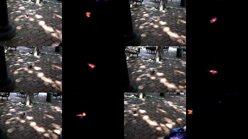
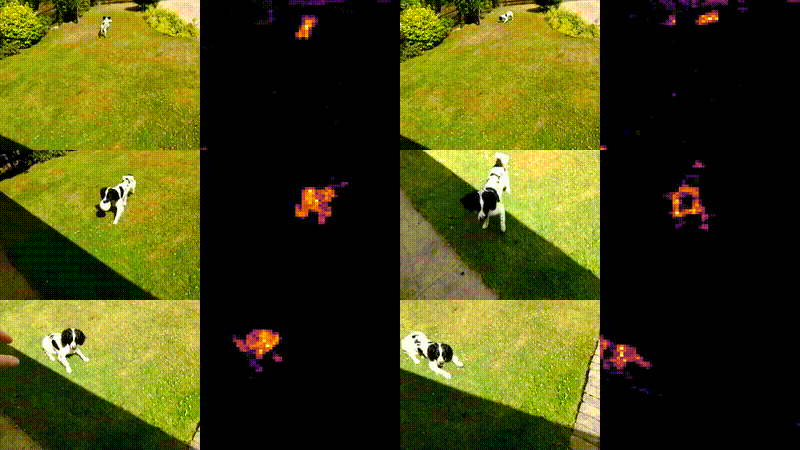
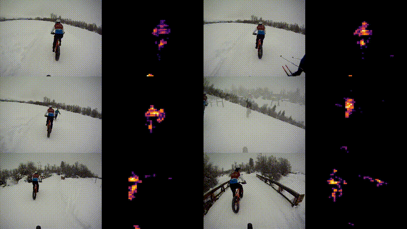
Demo
 |  |
 |  |
| shots | model | params | pretrain | epochs | DTD | aircr. | cars | cifar10 | cifar100 | flowers102 | food | pets | avg. |
|---|---|---|---|---|---|---|---|---|---|---|---|---|---|
| 1 | LeJEPA ViT-L | 304M | IN-1K | 100 | 33.21 | 9.37 | 3.40 | 51.65 | 27.01 | 48.53 | 17.14 | 46.11 | 29.55 |
| 1 | LeJEPA ConvNeXtV2-H | 660M | IN-1K | 100 | 32.15 | 8.07 | 4.28 | 50.95 | 31.48 | 48.74 | 17.95 | 58.98 | 31.58 |
| 1 | I-JEPA ViT-H | 632M | IN-1K | 300 | 27.71 | 9.86 | 4.33 | 56.52 | 30.58 | 44.69 | 14.53 | 53.38 | 30.20 |
| 10 | LeJEPA ViT-L | 304M | IN-1K | 100 | 64.72 | 35.25 | 22.25 | 85.15 | 59.77 | 92.53 | 50.90 | 77.00 | 60.95 |
| 10 | LeJEPA ConvNeXtV2-H | 660M | IN-1K | 100 | 61.84 | 30.67 | 24.46 | 85.74 | 63.29 | 91.78 | 49.32 | 78.53 | 60.70 |
| 10 | I-JEPA ViT-H | 632M | IN-1K | 300 | 57.68 | 33.82 | 21.96 | 88.77 | 66.42 | 88.24 | 43.97 | 83.23 | 60.51 |
| all | LeJEPA ViT-L | 304M | IN-1K | 100 | 78.30 | 57.01 | 57.28 | 96.50 | 83.71 | 91.21 | 82.05 | 89.74 | 79.48 |
| all | LeJEPA ConvNeXtV2-H | 660M | IN-1K | 100 | 76.60 | 52.99 | 54.88 | 96.15 | 81.34 | 91.11 | 77.64 | 89.76 | 77.56 |
| all | I-JEPA ViT-H | 632M | IN-1K | 300 | 73.32 | 56.61 | 54.47 | 97.54 | 86.42 | 86.47 | 81.02 | 92.11 | 78.50 |
Overview
LeJEPA is a lean, scalable, and theoretically grounded framework for self-supervised representation learning, based on Joint-Embedding Predictive Architectures (JEPAs). LeJEPA introduces Sketched Isotropic Gaussian Regularization (SIGReg), a novel objective that constrains learned embeddings to an optimal isotropic Gaussian distribution, minimizing downstream prediction risk. Key Features:
- Single trade-off hyperparameter
- Linear time and memory complexity
- Stable training across architectures and domains
- Heuristics-free implementation (no stop-gradient, teacher–student, or schedulers)
- Distributed training-friendly codebase (~50 lines of core code)
- State-of-the-art results across 10+ datasets and 60+ architectures
GOTO hyperparameters
Our data augmentation strategy follows a multi-crop approach inspired by DINO, where we generate multiple views of each image at different scales to encourage the model to learn both global semantic information and local fine-grained features.
Data augmentation and views
Each training image is augmented to produce 2 global views and 6 local views with different spatial scales but the same set of color and geometric transformations:
| Global Views | Local Views |
|---|---|
| RandomResizedCrop - Resolution: 224x224 - Scale: (0.3, 1.0) - Covers 30-100% of the image | RandomResizedCrop - Resolution: 98x98 - Scale: (0.05, 0.3) - Covers 5-30% of the image |
| RandomHorizontalFlip (p=0.5) | RandomHorizontalFlip (p=0.5) |
| ColorJitter (p=0.8) - Brightness: 0.4 - Contrast: 0.4 - Saturation: 0.2 - Hue: 0.1 | ColorJitter (p=0.8) - Brightness: 0.4 - Contrast: 0.4 - Saturation: 0.2 - Hue: 0.1 |
| RandomGrayscale (p=0.2) | RandomGrayscale (p=0.2) |
| GaussianBlur (p=0.5) | GaussianBlur (p=0.5) |
| RandomSolarize (p=0.2, threshold=128) | RandomSolarize (p=0.2, threshold=128) |
| Normalization (mean, std) | Normalization (mean, std) |
The key difference between global and local views is the cropping scale: global views capture larger portions of the image to learn high-level semantics, while local views focus on smaller regions to learn fine-grained local patterns. All other augmentations are applied identically to both view types to ensure consistency in the learned representations.
Training Configuration
We use the AdamW optimizer for all models and datasets with the following hyperparameters:
- Learning Rate:
5e-4(good starting point) - Weight Decay:
5e-2for Vision Transformers (ViT)5e-4for ResNets
- Precision: All training is performed using bfloat16 (bf16) mixed precision
- Learning Rate Schedule: Linear warmup with cosine annealing decay
- Final learning rate:
initial_lr / 1000
- Final learning rate:
Linear Probe Evaluation
For linear probe evaluation, we use the following configuration across all models (ours and baselines):
- Feature Extraction: Concatenation of the CLS token from the last two layers
- For ViT models without CLS token, we average all patch tokens (standard practice)
- Normalization: We apply LayerNorm or BatchNorm on the concatenated CLS tokens
- Following DINO, we found this improves linear probe performance in some settings
- No clear difference observed between LayerNorm and BatchNorm, so we used LayerNorm consistently
- Optimizer: AdamW (no significant difference found with SGD)
- Weight Decay:
1e-6(very small) - Learning Rate Schedule: Same as pre-training (linear warmup with cosine annealing)
Installation
LeJEPA is built on PyTorch and standard scientific Python libraries (e.g., NumPy). For rapid experimentation, we provide a pretraining skeleton script using stable_pretraining, a PyTorch Lightning wrapper. The core SIGReg loss can be integrated into any pretraining codebase.
Requirements:
- Python ≥ 3.8
- PyTorch ≥ 1.10
- NumPy
- (Optional)
stable_pretrainingfor provided training scripts Install via pip:
pip install lejepa
Quick Start: Using SIGReg
LeJEPA provides a variety of univariate and multivariate statistical tests for regularizing embeddings. Here is a minimal example using the SIGReg loss:
import lejepa

# Choose a univariate test (Epps-Pulley in this example)
univariate_test = lejepa.univariate.EppsPulley(num_points=17)

# Create the multivariate slicing test
loss_fn = lejepa.multivariate.SlicingUnivariateTest(
    univariate_test=univariate_test,
    num_slices=1024
)

# Compute the loss (embeddings: [num_samples, num_dims])
loss = loss_fn(embeddings)
loss.backward()
Citation
If you use LeJEPA in your research, please cite:
@misc{balestriero2025lejepaprovablescalableselfsupervised,
      title={LeJEPA: Provable and Scalable Self-Supervised Learning Without the Heuristics},
      author={Randall Balestriero and Yann LeCun},
      year={2025},
      eprint={2511.08544},
      archivePrefix={arXiv},
      primaryClass={cs.LG},
      url={https://arxiv.org/abs/2511.08544},
}
Contact & Contributions
We welcome issues, feature requests, and pull requests! For questions or collaborations, please contact rbalestr@brown.edu
Contributors

1 commits
Similar repos


Languages
Python
100.0%
README
LeJEPA
Lean Joint-Embedding Predictive Architecture (LeJEPA): Provable and Scalable Self-Supervised Learning Without the Heuristics
GitHub Repository
arXiv:2511.08544
Rush to our minimal working example to see a full-fledge working example (ViT, inet).
Demo
| |
| |
| shots | model | params | pretrain | epochs | DTD | aircr. | cars | cifar10 | cifar100 | flowers102 | food | pets | avg. |
|---|---|---|---|---|---|---|---|---|---|---|---|---|---|
| 1 | LeJEPA ViT-L | 304M | IN-1K | 100 | 33.21 | 9.37 | 3.40 | 51.65 | 27.01 | 48.53 | 17.14 | 46.11 | 29.55 |
| 1 | LeJEPA ConvNeXtV2-H | 660M | IN-1K | 100 | 32.15 | 8.07 | 4.28 | 50.95 | 31.48 | 48.74 | 17.95 | 58.98 | 31.58 |
| 1 | I-JEPA ViT-H | 632M | IN-1K | 300 | 27.71 | 9.86 | 4.33 | 56.52 | 30.58 | 44.69 | 14.53 | 53.38 | 30.20 |
| 10 | LeJEPA ViT-L | 304M | IN-1K | 100 | 64.72 | 35.25 | 22.25 | 85.15 | 59.77 | 92.53 | 50.90 | 77.00 | 60.95 |
| 10 | LeJEPA ConvNeXtV2-H | 660M | IN-1K | 100 | 61.84 | 30.67 | 24.46 | 85.74 | 63.29 | 91.78 | 49.32 | 78.53 | 60.70 |
| 10 | I-JEPA ViT-H | 632M | IN-1K | 300 | 57.68 | 33.82 | 21.96 | 88.77 | 66.42 | 88.24 | 43.97 | 83.23 | 60.51 |
| all | LeJEPA ViT-L | 304M | IN-1K | 100 | 78.30 | 57.01 | 57.28 | 96.50 | 83.71 | 91.21 | 82.05 | 89.74 | 79.48 |
| all | LeJEPA ConvNeXtV2-H | 660M | IN-1K | 100 | 76.60 | 52.99 | 54.88 | 96.15 | 81.34 | 91.11 | 77.64 | 89.76 | 77.56 |
| all | I-JEPA ViT-H | 632M | IN-1K | 300 | 73.32 | 56.61 | 54.47 | 97.54 | 86.42 | 86.47 | 81.02 | 92.11 | 78.50 |
Overview
LeJEPA is a lean, scalable, and theoretically grounded framework for self-supervised representation learning, based on Joint-Embedding Predictive Architectures (JEPAs). LeJEPA introduces Sketched Isotropic Gaussian Regularization (SIGReg), a novel objective that constrains learned embeddings to an optimal isotropic Gaussian distribution, minimizing downstream prediction risk. Key Features:
- Single trade-off hyperparameter
- Linear time and memory complexity
- Stable training across architectures and domains
- Heuristics-free implementation (no stop-gradient, teacher–student, or schedulers)
- Distributed training-friendly codebase (~50 lines of core code)
- State-of-the-art results across 10+ datasets and 60+ architectures
GOTO hyperparameters
Our data augmentation strategy follows a multi-crop approach inspired by DINO, where we generate multiple views of each image at different scales to encourage the model to learn both global semantic information and local fine-grained features.
Data augmentation and views
Each training image is augmented to produce 2 global views and 6 local views with different spatial scales but the same set of color and geometric transformations:
| Global Views | Local Views |
|---|---|
| RandomResizedCrop - Resolution: 224x224 - Scale: (0.3, 1.0) - Covers 30-100% of the image | RandomResizedCrop - Resolution: 98x98 - Scale: (0.05, 0.3) - Covers 5-30% of the image |
| RandomHorizontalFlip (p=0.5) | RandomHorizontalFlip (p=0.5) |
| ColorJitter (p=0.8) - Brightness: 0.4 - Contrast: 0.4 - Saturation: 0.2 - Hue: 0.1 | ColorJitter (p=0.8) - Brightness: 0.4 - Contrast: 0.4 - Saturation: 0.2 - Hue: 0.1 |
| RandomGrayscale (p=0.2) | RandomGrayscale (p=0.2) |
| GaussianBlur (p=0.5) | GaussianBlur (p=0.5) |
| RandomSolarize (p=0.2, threshold=128) | RandomSolarize (p=0.2, threshold=128) |
| Normalization (mean, std) | Normalization (mean, std) |
The key difference between global and local views is the cropping scale: global views capture larger portions of the image to learn high-level semantics, while local views focus on smaller regions to learn fine-grained local patterns. All other augmentations are applied identically to both view types to ensure consistency in the learned representations.
Training Configuration
We use the AdamW optimizer for all models and datasets with the following hyperparameters:
- Learning Rate:
5e-4(good starting point) - Weight Decay:
5e-2for Vision Transformers (ViT)5e-4for ResNets
- Precision: All training is performed using bfloat16 (bf16) mixed precision
- Learning Rate Schedule: Linear warmup with cosine annealing decay
- Final learning rate:
initial_lr / 1000
- Final learning rate:
Linear Probe Evaluation
For linear probe evaluation, we use the following configuration across all models (ours and baselines):
- Feature Extraction: Concatenation of the CLS token from the last two layers
- For ViT models without CLS token, we average all patch tokens (standard practice)
- Normalization: We apply LayerNorm or BatchNorm on the concatenated CLS tokens
- Following DINO, we found this improves linear probe performance in some settings
- No clear difference observed between LayerNorm and BatchNorm, so we used LayerNorm consistently
- Optimizer: AdamW (no significant difference found with SGD)
- Weight Decay:
1e-6(very small) - Learning Rate Schedule: Same as pre-training (linear warmup with cosine annealing)
Installation
LeJEPA is built on PyTorch and standard scientific Python libraries (e.g., NumPy). For rapid experimentation, we provide a pretraining skeleton script using stable_pretraining, a PyTorch Lightning wrapper. The core SIGReg loss can be integrated into any pretraining codebase.
Requirements:
- Python ≥ 3.8
- PyTorch ≥ 1.10
- NumPy
- (Optional)
stable_pretrainingfor provided training scripts Install via pip:
pip install lejepa
Quick Start: Using SIGReg
LeJEPA provides a variety of univariate and multivariate statistical tests for regularizing embeddings. Here is a minimal example using the SIGReg loss:
import lejepa

# Choose a univariate test (Epps-Pulley in this example)
univariate_test = lejepa.univariate.EppsPulley(num_points=17)

# Create the multivariate slicing test
loss_fn = lejepa.multivariate.SlicingUnivariateTest(
    univariate_test=univariate_test,
    num_slices=1024
)

# Compute the loss (embeddings: [num_samples, num_dims])
loss = loss_fn(embeddings)
loss.backward()
Citation
If you use LeJEPA in your research, please cite:
@misc{balestriero2025lejepaprovablescalableselfsupervised,
      title={LeJEPA: Provable and Scalable Self-Supervised Learning Without the Heuristics},
      author={Randall Balestriero and Yann LeCun},
      year={2025},
      eprint={2511.08544},
      archivePrefix={arXiv},
      primaryClass={cs.LG},
      url={https://arxiv.org/abs/2511.08544},
}
Contact & Contributions
We welcome issues, feature requests, and pull requests! For questions or collaborations, please contact rbalestr@brown.edu
Similar repos
Contributors
1 commits
Languages
Python
100.0%