Repository for the "Discovering Functionally Selective Brain Regions with a Deep Topographic Multimodal Model" paper
Python
7
28 commits
updated Sep 25, 2026



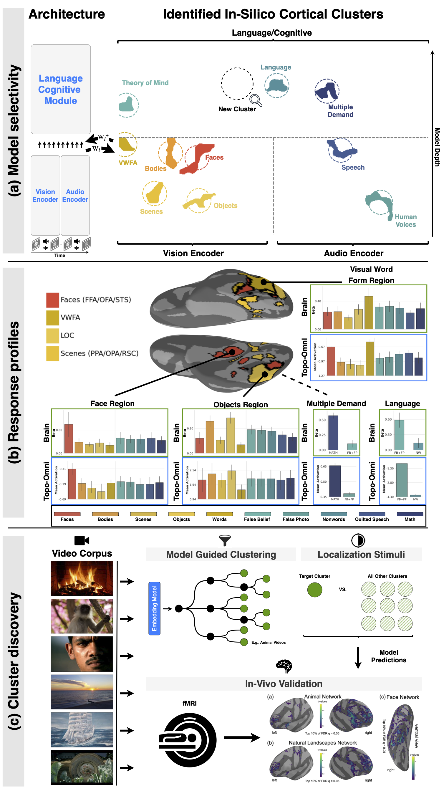
Inducing topographic organization in a multimodal language model (Qwen2.5-Omni) using a spatial smoothness loss inspired by biological cortical maps.
The model learns a 2-D cortical sheet, a fixed spatial layout of neurons shared across all transformer layers, and is trained to encourage nearby neurons to respond similarly. The result is emergent functional regions (face patches, scene areas, auditory regions) that spatially cluster on the sheet, mirroring organization in the human brain.
Standard neural networks have no spatial structure: any neuron can interact with any other regardless of position. The brain, by contrast, organizes neurons topographically: neurons with similar tuning are physically close. TopoOmni injects this inductive bias into Qwen2.5-Omni-3B by:
The approach builds on TDANN and TopoLM.
topo-omni/
├── make_all_figures.py          # orchestrator: reproduce all model-side figures (precomputed|raw)
├── download_precomputed.py      # fetch the precomputed cut from OSF (+ sha256 verify)
├── .env.example                 # environment template (copy to .env)
├── src/
│   │                             # Shared library first, then one folder per experiment.
│   ├── core/
│   │   ├── model_loading.py      # load_topo_omni(): single HuggingFace/local model loader
│   │   └── precomputed.py        # OSF cut fetch + sha256 verify
│   ├── models/
│   │   ├── qwen2_5_omni.py       # Modified Qwen2.5-Omni with cortical sheet output
│   │   └── spatial_utils.py      # LayerPositions, spatial loss, neighborhood utilities
│   ├── utils/                    # Sheet-generic numerics, shared across experiments
│   │   ├── smoothing.py          # Gaussian smoothing over the cortical sheet
│   │   ├── spatial_stats.py      # Selectivity / spatial-statistics helpers
│   │   ├── connected_components.py
│   │   └── island_morans_I.py    # Spatial autocorrelation (Moran's I) for patchy maps
│   ├── training/                 # Everything needed to TRAIN a model (run from src/)
│   │   ├── train.py              # Training entry point
│   │   ├── distill.py            # Knowledge distillation entry point
│   │   ├── init_coords.py        # Pre-compute cortical coords / neighborhood structures
│   │   ├── data_utils.py         # Dataset loading and collation
│   │   └── batching.py           # Modality-homogeneous batch sampler
│   ├── configs/
│   │   ├── accelerate.yml        # Accelerate/DeepSpeed launcher config
│   │   ├── init/                 # Cortical coordinate initialization (coords*.yml)
│   │   ├── train/                # Training configs (base.yml, tiled32_4608.yml, ...)
│   │   └── eval/                 # Eval configs (retinotopy.yml, tonotopy.yml, marvi.yml, ...)
│   ├── experiments/              # ONE FOLDER PER EXPERIMENT — each holds the whole chain
│   │   │                         # (extract → run → analyse → plot) for that phenomenon.
│   │   ├── orientation/          # Orientation maps, pinwheels, column spacing (Lambda)
│   │   │   ├── run.py            #   map orientation preference over the sheet
│   │   │   ├── metrics.py        #   preferred orientation, OSI, pinwheel detection
│   │   │   ├── reference.py      #   reference-map construction
│   │   │   ├── measure_lambda.py #   column spacing per vision-encoder tile
│   │   │   ├── pinwheel_null.py  #   pinwheel count vs shuffled null
│   │   │   ├── pinwheel_scan.py  #   scan slot ranges for pinwheel excess
│   │   │   ├── plot_panel.py     #   paper panel: smoothed orientation map
│   │   │   ├── plot_tiled.py     #   per-slot maps for a tiled sheet
│   │   │   ├── plot_density_bars.py
│   │   │   ├── smoothness_panels.py, smoothness_window_scan.py
│   │   │   ├── tangential_ratio.py, nn_delta.py, deep_band_continuous.py
│   │   │   └── macaque_map.py, tdann_model.py   # macaque V1 + TDANN references
│   │   ├── retinotopy/
│   │   │   ├── stimuli.py        #   localized stimulus bank (self-generating)
│   │   │   ├── run.py            #   retinotopic mapping
│   │   │   └── run_angle.py, run_ecc.py         # polar angle / eccentricity
│   │   ├── tonotopy/
│   │   │   ├── stimuli.py        #   pure-tone stimulus bank
│   │   │   ├── run.py            #   tonotopic mapping
│   │   │   └── plot.py
│   │   ├── selectivity/          # Category selectivity over the sheet
│   │   │   ├── extract_features.py  # model responses to localizer stimuli
│   │   │   ├── run.py            #   ON vs OFF t-contrast, FDR-corrected
│   │   │   ├── plot.py           #   in-silico selectivity sheet
│   │   │   └── topo_nontopo.py, topo_nontopo_clustering.py  # topo vs non-topo controls
│   │   ├── response_profiles/    # Per-category response bars (model vs fMRI localizers)
│   │   │   ├── cognitive.py, marvi.py           # compute profiles
│   │   │   └── plot.py, plot_cognitive.py, plot_pernet.py
│   │   ├── ablation/             # Causal tests: ablation + stimulation
│   │   │   ├── run.py            #   ablate a sheet region, measure behaviour
│   │   │   ├── plot.py, plot_barplot.py
│   │   │   ├── similarity.py, no_ablation_judge.py
│   │   │   └── stimulation_perception.py, driving_perception.py
│   │   ├── spacetop_discovery/   # Model-guided discovery of novel networks (SpaceTop)
│   │   │   ├── extract.py, extract_rating.py
│   │   │   ├── contrast.py       #   cluster contrasts
│   │   │   ├── run_clusters_iou.py, explore_cluster_iou.py   # IoU vs null
│   │   │   ├── plot_selectivity.py, plot_corr.py
│   │   │   ├── correlate_t_values.py            # model vs fMRI t-maps
│   │   │   │                     # unsupervised discovery chain (was topo-discover/):
│   │   │   ├── extract_video_embeddings.py, compile_embeddings.py   # per-clip embeddings
│   │   │   ├── agglomerative_early_stopping.py, merge_clusters.py,  # cluster
│   │   │   │   plot_dendrogram.py
│   │   │   └── create_cluster_manifest.py, calculate_selectivity.py, # label + inspect
│   │   │       plot_model_selectivity.py, make_cluster_collages.py
│   │   └── brain_alignment/      # Encoding-model alignment to human fMRI
│   │       ├── plot_barplot.py
│   │       └── table.py, table_stats.py
│   ├── tools/                    # Dev/preflight utilities (not part of the paper pipeline)
│   ├── ckpts -> ../artifacts/ckpts              # symlinks; real dirs live in artifacts/
│   ├── neighborhoods -> ../artifacts/neighborhoods
│   └── wandb -> ../artifacts/wandb
├── artifacts/                    # Gitignored run outputs: checkpoints, neighborhoods, wandb logs
├── scripts/                      # Shell launchers, batch sweeps, result-compilation utilities
│   ├── reproduce_precomputed_figures.sh  # one-command precomputed reproduction
│   ├── train.sh
│   ├── run_ablation.sh
│   ├── run_iou.sh
│   ├── marvi_response_profiles.sh
│   ├── cognitive_response_profiles.sh
│   ├── pernet_response_profiles.sh
│   ├── plot_spacetop.sh
│   ├── compile_iou.py
│   ├── compile_moran_I.py
│   ├── run_selectivity.py        # Batch launcher for selectivity sweeps
│   ├── submit_train.py
│   ├── submit_topoomni_ablation.sh
│   ├── submit_topoomni_spacetop_discovery.sh
│   ├── submit_topoomni_stimulation.sh
│   └── figures/                  # Scripts that reproduce individual paper figures
├── data/                         # Small tracked artifacts (summary CSVs, figures);
│                                 # large stimuli/checkpoints/datasets are gitignored
├── fMRI/                         # ⚠ SEPARATE SUBPROJECT — brain-side, not the model.
│                                 # Reanalyzes the 3 human-fMRI datasets (Pernet/Marvi/Jung) to
│                                 # reproduce the paper's brain figures from a precomputed OSF cut.
│                                 # Own Nilearn stack + per-dataset envs (no torch/transformers);
│                                 # shares dataset names with src/ but no data or code. See below.
├── requirements.txt
└── README.md
Each paper figure is reproduced by one script in scripts/figures/, which shells out to the
experiment folders under src/experiments/. To follow a figure back to its source, start here:
| Figure | Reproduce with | Experiment folder(s) |
|---|---|---|
| 1a | scripts/figures/figure_1a.py | experiments/selectivity/ — unified sheet, tiled32 run |
| 2c | scripts/figures/figure_2.py | experiments/spacetop_discovery/ |
| 3 | scripts/figures/figure_3.py | experiments/selectivity/, experiments/response_profiles/, experiments/retinotopy/ |
| 4 | scripts/figures/figure_4.py | experiments/tonotopy/, experiments/response_profiles/ |
| 5 | scripts/figures/figure_5.py | experiments/response_profiles/ |
| 6 | scripts/figures/figure_6.py | experiments/ablation/ |
| 7 | scripts/figures/figure_7.py | experiments/spacetop_discovery/ |
Figure 1a is the only figure built on the topo-omni-tiled32-4608 run (800x576 sheet); every
other figure uses the default topo-omni strip model. Its selectivity stats are the one expensive
input: 10 localizers x a model load each. Either run them sequentially
python scripts/run_selectivity.py --model_name topo-omni-tiled32-4608 --fwhm 3.0
or restrict it to a subset of localizers:
python scripts/run_selectivity.py --model_name topo-omni-tiled32-4608 --fwhm 3.0 \
    --conditions faces,scenes
To fan out across the cluster instead, submit that same command once per localizer as
its own single-GPU runai job (A100 default pool) — no wrapper script ships with
the repo. run_selectivity.py tags each job's transient eval config with a uuid, so
concurrent jobs sharing the NFS checkout cannot clobber one another's config.
Both write results/topo-omni-tiled32-4608/<localizer>/<localizer>_fwhm3.0_selectivity_stats.pkl,
which is what scripts/figures/figure_1a.py reads.
Supporting analyses that are not a single main-text figure live in
experiments/orientation/ (orientation maps, pinwheels, column spacing) and
experiments/brain_alignment/ (encoding-model alignment tables).
Every experiment folder holds the whole chain for that phenomenon — feature extraction,
the run/eval step, post-hoc analysis, and plotting — so nothing has to be traced across
run/, extract/, analysis/, and visualize/ directories any more.
The cortical sheet is a 304 × 512 2-D grid that spans the entire model:
| Rows | Component |
|---|---|
| 0 – 159 | Vision encoder layers |
| 0 – 159 (cols 256–511) | Audio encoder layers |
| 160 – 303 | Thinker (LM) layers |
Each unit (neuron) has a fixed coordinate on this grid. The spatial loss computes pairwise response similarity within local Chebyshev-distance neighborhoods and penalizes dissimilarity between neighbors. The loss weight alpha (default: 20) controls how strongly the spatial constraint is applied relative to the task loss.
pip install -r requirements.txt
Copy .env.example to .env at the repo root (loaded via python-dotenv) and fill in the paths
you need. For the default figure-reproduction path (precomputed) you need none of them — only
SAVE_DIR (where the downloaded cut lands) is used, and the reproduce script sets it for you. The
other paths matter only for the raw recompute path and for training. The trained model is loaded
from HuggingFace (epfl-neuroai/topo-omni) by default, so no checkpoint download is required.
Operating system. Developed and tested on Ubuntu Linux 22.04 (x86_64). The code is standard cross-platform Python but has only been tested on Linux.
Python. Python 3.10.
Software dependencies. All Python dependencies, with pinned versions, are listed in
requirements.txt and installed with the command in Setup. Key packages:
torch, transformers, trl, accelerate, deepspeed, qwen_omni_utils, omegaconf, wandb,
plus numpy, scipy, scikit-learn and matplotlib. The brain-side fMRI/ subproject has
its own separate Nilearn-based environment (see fMRI/README.md).
Tested on. Ubuntu Linux, Python 3.10, with the package versions pinned in requirements.txt.
Typical install time. A few minutes on a normal desktop (~5–15 minutes), dominated by downloading the PyTorch / CUDA wheels.
Hardware.
accelerate + deepspeed.No other non-standard hardware is required.
The model-side figure panels (Fig 2b/c, 3, 4, 5, 6, 7) reproduce via two clearly separated
paths, mirroring the brain-side fMRI/ subproject — see docs/DESIGN.md
for the rationale and a per-panel input-availability table.
1. Precomputed (default, recommended) — plot from a hosted cut of model outputs. No GPU, no stimuli, no model download.
./scripts/reproduce_precomputed_figures.sh            # download cut from OSF + render all figures
./scripts/reproduce_precomputed_figures.sh 3 4        # a subset

# …or the two steps by hand:
python download_precomputed.py --dest _precomputed_cut
python make_all_figures.py --input-source precomputed --derivatives-root _precomputed_cut
Panels land in figures_out/figure_<id>/.
This precomputed path also serves as the demo required by the software checklist. It runs on a small hosted cut of model outputs (downloaded from OSF), needs no GPU, no stimuli and no model download.
- Demo dataset: the precomputed cut fetched by
download_precomputed.pyfrom OSF (DOI 10.17605/OSF.IO/EHRT6).- Expected output: rendered panels written to
figures_out/figure_<id>/(e.g.figures_out/figure_3/).- Expected run time: roughly ~5 minutes on a normal desktop for the full set (less for a subset such as
./scripts/reproduce_precomputed_figures.sh 3 4).
2. Raw (opt-in) — download the model from HuggingFace and recompute from stimuli (needs a GPU).
Fully wired where inputs are public (the retinotopy/tonotopy stimulus banks self-generate); panels
whose localizer stimuli aren't redistributable read from a STIMULI_DIR you supply.
python make_all_figures.py --input-source raw --derivatives-root results --figures 3,4
Everything below documents the individual building blocks these two paths orchestrate.
Evaluation / figure commands are run from the repo root (module form, e.g.
python -m src.experiments.<topic>.<script>). The training commands (steps 1–2) are run from inside src/.
Pre-computes neighborhood structures for the spatial loss. Run once before training.
cd src && python training/init_coords.py --config configs/init/coords.yml
This generates .pkl files under src/neighborhoods/ (a symlink to artifacts/neighborhoods/) keyed by model name, radius, and neighborhood count.
cd src && bash ../scripts/train.sh train/base.yml <num_gpus> accelerate.yml
Key config options (configs/train/base.yml):
| Key | Default | Description |
|---|---|---|
train.apply-spatial-loss | true | Enable the topographic loss |
topo-params.alpha | 20 | Spatial loss weight |
topo-params.position-dir | neighborhoods/... | Pre-computed neighborhood directory |
topo-params.cortical-init | 0.001 | Cortical output projection init scale |
topo-params.identity-init | true | Initialize output projection as identity |
train.n-epochs | 5 | Training epochs |
train.batch-size | 4 | Per-device batch size |
train.grad-accum | 4 | Gradient accumulation steps |
train.learning-rate | 5e-5 | Learning rate |
Training logs to Weights & Biases when --wandb is passed.
Tests whether specific regions on the cortical sheet are selective for a category (faces, bodies, objects, scenes, speech, etc.) versus control stimuli.
python -m src.experiments.selectivity.run --config src/configs/eval/marvi.yml
The model is loaded from HuggingFace (epfl-neuroai/topo-omni) by default; set $TOPO_OMNI_MODEL
or model.model in the config to use a local checkpoint instead.
Key config options (src/configs/eval/marvi.yml):
| Key | Description |
|---|---|
model.model | (optional) HF id or local checkpoint dir (default: $TOPO_OMNI_MODEL) |
data.mode | video, image, or text |
data.stimuli_root | Path to ON/OFF stimuli folders |
data.lm_reduce | Reduction over LM sheet (mean/max) |
stats.alpha | p-value threshold for selectivity |
stats.smooth | Apply Gaussian smoothing before testing |
stats.fwhm_mm | Smoothing kernel FWHM (mm) |
Ablates (zeros out) or stimulates (amplifies) a localizer-defined region and measures the effect on downstream responses.
bash scripts/run_ablation.sh
Extract model activations for NSD (images) or SpaceTop (videos) fMRI datasets, then compare the topographic layout to human brain responses.
# NSD
python -m src.experiments.selectivity.extract_features

# SpaceTop
python -m src.experiments.spacetop_discovery.extract --group-index 0
Run correlation analysis:
python -m src.experiments.spacetop_discovery.contrast --cluster_id 32 --topk 1
Compute and plot how the top-k% most selective neurons respond across all stimulus categories. Separate sweeps are provided per localizer family:
bash scripts/marvi_response_profiles.sh [top_k_pct] [fwhm_mm] [anatomical_constraint]      # faces, scenes, objects, vwfa, bodies, speech
bash scripts/cognitive_response_profiles.sh [top_k_pct] [fwhm_mm]                          # language, theory of mind, multiple demand
bash scripts/pernet_response_profiles.sh [top_k_pct] [fwhm_mm] [anatomical_constraint]     # PerNet vocal/non-vocal folds
These call into experiments/response_profiles/marvi.py / experiments/response_profiles/cognitive.py and plot via experiments/response_profiles/plot.py, experiments/response_profiles/plot_cognitive.py, and experiments/response_profiles/plot_pernet.py.
Map preferred visual-field position (eccentricity / polar angle) and preferred sound frequency across the cortical sheet, masking units that fail an ANOVA tuning test (FDR-corrected). The stimulus banks self-generate (no data download), which makes these panels fully reproducible on the raw path with only a GPU:
# 1. generate the (public) stimulus banks into $STIMULI_DIR
python -m src.experiments.retinotopy.stimuli     # -> $STIMULI_DIR/retino_bank/{*.png, manifest.csv}
python -m src.experiments.tonotopy.stimuli    # -> $STIMULI_DIR/tone_bank/{*.wav, manifest.csv}

# 2. run the model over them (produces the maps directly)
python -m src.experiments.retinotopy.run --config src/configs/eval/retinotopy.yml   # polar angle + eccentricity
python -m src.experiments.tonotopy.run   --config src/configs/eval/tonotopy.yml     # preferred frequency
(The single-axis variants run_retinotopy_ecc / run_retinotopy_angle expect eccentricity/ and angle/ sub-banks instead of the combined retino_bank.)
The same masked-map treatment is available for orientation preference, using the TDANN orientation-bias sine-grating bank (510 full-field gratings: 8 orientations x 8 spatial frequencies x 5 phases x {bw, rg}). That bank is not self-generating, but it is public, so the script downloads it from OSF on first run — no manual staging:
python -m src.experiments.orientation.run --config src/configs/eval/orientation.yml
It writes a preferred-orientation map (cyclic colormap), an orientation-selectivity-index (OSI) map, a scatter over the whole sheet, and a histogram of preferred orientations against the bank's own orientation distribution. Each unit's opacity encodes how strongly it is tuned, so marginal units fade into the background instead of being shown or hidden by a flat pass/fail mask.
stats.criterion selects what "tuned" means — all three are computed and saved every run, so switching only re-renders the figures:
| criterion | statistic | default cutoff |
|---|---|---|
reliability (default) | correlation between tuning curves from two halves of the stimuli, split along a nuisance dimension (stats.reliability_split: sf, phase, colour, random) | 0.5 |
eta2 | fraction of the unit's response variance explained by orientation | 0.10 |
fdr | FDR-corrected ANOVA p-value | stats.alpha |
Prefer reliability or eta2 over fdr. A p-value needs an absurd threshold here (~1e-50) to be selective, and the multiple-comparisons correction is not the reason: measured on this sheet, the whole span from uncorrected p to Bonferroni is 5.2 orders of magnitude — necessarily log10 of the 155,648 tests — so no correction moves the threshold far, and even Bonferroni still leaves ~82% of the vision band significant at 0.05. What actually inflates p is (i) the model being deterministic, so the ANOVA's error term is nuisance variance rather than trial noise and "the orientation effect is exactly zero" is essentially never true, and (ii) running the test on the smoothed sheet, worth ~13 orders of magnitude at the median (49% → 99% of the band significant) because near-silent units inherit their neighbours' tuning. Corrections that model the smoothing-induced dependence (RFT, cluster permutation) make the threshold more lenient, not less. A tiny alpha is an effect-size filter in disguise, so use an effect size.
To quantify the resulting map with the metrics TDANN reports for V1 (Margalit et al.,
Fig. 2 / notebooks/F02_V1_Details):
python -m src.experiments.orientation.metrics
This reads the orientation_stats.npz the run above wrote — no GPU, no re-extraction — and
reports circular variance (CV = 1 - |R|, identical to 1 - OSI), column spacing
Λ (from the peak of the radially averaged power spectrum of exp(2iθ); TDANN hard-codes
this per model, we estimate it), pinwheel density in pinwheels per Λ² (winding numbers
over the smoothed map, then connected-component counting — dimensionless, so comparable to
TDANN's ~2.1 and macaque V1's ~3.0), and map smoothness ((max - first) / max of the
Δ-preferred-orientation-vs-distance curve).
Two caveats it prints and you should not skip:
--smooth-window-frac 0.15)
keeps ~16 px per Λ, and the script warns below 8 px per Λ.
To compare the map against the reference data TDANN uses:python -m src.experiments.orientation.reference
The reference is macaque V1, not human. TDANN's Fig. 2 compares against macaque
optical-imaging maps (Nauhaus) and macaque single units (Ringach et al. 2002); human V1
orientation columns have never been mapped at pinwheel resolution, so there is no human
reference for these metrics. (The human fMRI data under fMRI/ is category
selectivity, not orientation, and cannot substitute.)
Two reference curves are reconstructed rather than read off a figure:
data/ringach_2002_db.mat (shipped by TDANN) holds the real
per-neuron values, so the script runs an actual two-sample KS test.experiments/orientation/macaque_map.py reproduces TDANN's
NauhausOrientationTissue, which is not a data file: it colour-decodes the orientation
panel of Fig. 2 of Nauhaus et al. (2012, Nat Neurosci 15:1683) against that panel's own
legend, and scales pixels to mm with its scale bar. Our reconstruction yields macaque
smoothness 0.684 against TDANN's published ~0.65, which validates the port. The source
figure is copyrighted, so it is fetched on demand and gitignored; only the derived curve
(data/macaque_delta_curve.npz) is tracked.Smoothness is not parameter-free. It depends both on the smoothing fwhm used to build the
map (0.730 at fwhm=4 vs 0.466 at fwhm=2 on this sheet — straddling macaque's 0.684) and on the
distance binning, since (max - curve[0]) / max moves with the width of the first bin. The
metrics script therefore uses TDANN's own binning (9 bins reaching 0.943·Λ), and only values
computed at matched fwhm and matched bins should be compared.
Pinwheel density and the remaining panel values are still TDANN's Fig. 2 compares against macaque
optical-imaging maps (Nauhaus) and macaque single units (Ringach et al. 2002); human V1
orientation columns have never been mapped at pinwheel resolution, so there is no human
reference for these metrics. (The human fMRI data under fMRI/ is category
selectivity, not orientation, and cannot substitute.) Circular variance is a genuine
quantitative comparison — data/ringach_2002_db.mat ships the real per-neuron values, so
the script runs an actual two-sample KS test. Pinwheel density and smoothness references are
read off the published figure and labelled approximate, because TDANN does not
redistribute the macaque map data they come from.
Λ
and pinwheel density are not straightforwardly the V1 quantities. The script quantifies how
badly this bites: the map's anisotropy, and whether neighbouring rows are more alike within
a layer than across a layer boundary.For reliability, use a structured split rather than random: random halves draw the same mixture of nuisance stimuli and so only measure sampling noise — a unit whose preferred orientation shifts 45° between low and high spatial frequency still scores r ≈ 0.97. Splitting along sf instead asks whether the preference survives a change in spatial frequency, and on this sheet that drops median vision-band reliability from 0.87 to 0.58. Preference and OSI come from the circular (axial, mod-180°) vector average of each unit's tuning curve. Note the bank deliberately oversamples cardinal orientations (0°: 79 stimuli, 90°: 80, vs 45°: 47, 135°: 48); responses are averaged within each orientation before that vector average, which keeps the sampling bias out of the estimate (taking it over the raw stimuli instead shifts preferences by up to ~4°). The histogram overlay is what separates a genuine cardinal preference in the sheet from the bank's sampling bias.
Measure the spatial overlap (IoU) of thresholded activation masks across stimulus groups, with a random-sampling null distribution for significance.
bash scripts/run_iou.sh
| Metric | Script | Description |
|---|---|---|
| Selectivity (t-test) | experiments/selectivity/run.py | ON vs OFF contrast, FDR-corrected |
| Moran's I | utils/island_morans_I.py | Spatial autocorrelation of the selectivity map |
| Brain alignment (r) | experiments/spacetop_discovery/contrast.py | Correlation with fMRI t-maps |
| Ablation accuracy | experiments/ablation/similarity.py | Cross-category response similarity under ablation |
| Cluster IoU | experiments/spacetop_discovery/run_clusters_iou.py | Overlap of activation masks across groups |
| Retinotopic tuning | experiments/retinotopy/run*.py | Preferred eccentricity/polar-angle per unit, ANOVA-tested |
| Tonotopic tuning | experiments/tonotopy/run.py | Preferred sound frequency per unit, ANOVA-tested |
| Orientation tuning | experiments/orientation/run.py | Preferred orientation + OSI per unit (circular, mod-180°), ANOVA-tested |
| Orientation map structure | experiments/orientation/metrics.py | Circular variance, column spacing, pinwheel density, map smoothness (TDANN Fig. 2 metrics) |
| Orientation map vs. macaque | experiments/orientation/reference.py | KS of circular variance against Ringach 2002 macaque V1 (n=308) |
| Macaque reference map | experiments/orientation/macaque_map.py | Reconstructs TDANN's macaque orientation map to overlay its Δorientation-vs-distance curve |
src/experiments/spacetop_discovery/ runs an unsupervised pipeline to find functionally selective clusters from video-driven activations: extract per-clip embeddings (extract_video_embeddings.py, compile_embeddings.py), agglomeratively cluster them (agglomerative_early_stopping.py, plot_dendrogram.py, merge_clusters.py), then label and inspect the resulting clusters (create_cluster_manifest.py, calculate_selectivity.py, plot_model_selectivity.py, make_cluster_collages.py).
fMRI/)fMRI/ is a self-contained subproject and is quite different from the rest of this repository. Everything above (src/, scripts/) builds, trains, and analyzes the model; fMRI/ instead reanalyzes the human brain data. It holds the brain-side pipelines for the three human-fMRI datasets validated in the paper — Pernet 2015 (voice), Marvi 2025 (localizers), and Jung 2025 / SpaceTop (naturalistic movie) — reproducing the paper's brain figures. It has its own dependency stack (Nilearn — not torch/transformers), its own per-dataset conda environments, its own data (hosted on OSF, not in git), and its own docs; it shares only dataset names with src/, no data and no code. Each dataset runs a two-stage pipeline (Stage 0 preprocessing → Stage 1 analysis → figures) with two entry points — start from the hosted precomputed cut (default, recommended) or rebuild from raw scans (--input-source raw). Full setup + details: fMRI/README.md; design rationale: fMRI/docs/DESIGN.md.
Data and figures are not in git — the precomputed cut is hosted on OSF (umbrella https://osf.io/ehrt6/, DOI 10.17605/OSF.IO/EHRT6; one component per dataset, all public). make_all_figures.py renders from a cut that must already be on disk — it does not download or preprocess anything, so you must first either download the cut from OSF (download_precomputed.py) or produce it yourself via Stage-0 preprocessing (--input-source raw; see fMRI/README.md). Reproduce from a clean checkout:
cd fMRI
./reproduce_precomputed_figures.sh               # one command: download cut + render + fetch reference renders
# …or the two steps manually:
python download_precomputed.py --dest .          # STEP 1 — cut -> ./<Dataset>/  (public; no token needed)
python make_all_figures.py --derivatives-root .  # STEP 2 — figures -> ./<Dataset>/plots/  (needs STEP 1)
Runtime note: Jung and Pernet finish in minutes (Pernet needs a compute node with several GB RAM); Marvi can take multiple hours (its Branch-A fROI cross-validation). See fMRI/README.md → "Compute resources" for the RAM/core guide.
| Package | Role |
|---|---|
transformers | Qwen2.5-Omni base model |
trl | SFT training loop (SFTTrainer) |
accelerate + deepspeed | Multi-GPU training |
qwen_omni_utils | Multimodal preprocessing |
omegaconf | YAML config management |
wandb | Experiment tracking |
Repository for the "Discovering Functionally Selective Brain Regions with a Deep Topographic Multimodal Model" paper
Python
7
28 commits
updated Sep 25, 2026
Inducing topographic organization in a multimodal language model (Qwen2.5-Omni) using a spatial smoothness loss inspired by biological cortical maps.
The model learns a 2-D cortical sheet, a fixed spatial layout of neurons shared across all transformer layers, and is trained to encourage nearby neurons to respond similarly. The result is emergent functional regions (face patches, scene areas, auditory regions) that spatially cluster on the sheet, mirroring organization in the human brain.
Standard neural networks have no spatial structure: any neuron can interact with any other regardless of position. The brain, by contrast, organizes neurons topographically: neurons with similar tuning are physically close. TopoOmni injects this inductive bias into Qwen2.5-Omni-3B by:
The approach builds on TDANN and TopoLM.
topo-omni/
├── make_all_figures.py          # orchestrator: reproduce all model-side figures (precomputed|raw)
├── download_precomputed.py      # fetch the precomputed cut from OSF (+ sha256 verify)
├── .env.example                 # environment template (copy to .env)
├── src/
│   │                             # Shared library first, then one folder per experiment.
│   ├── core/
│   │   ├── model_loading.py      # load_topo_omni(): single HuggingFace/local model loader
│   │   └── precomputed.py        # OSF cut fetch + sha256 verify
│   ├── models/
│   │   ├── qwen2_5_omni.py       # Modified Qwen2.5-Omni with cortical sheet output
│   │   └── spatial_utils.py      # LayerPositions, spatial loss, neighborhood utilities
│   ├── utils/                    # Sheet-generic numerics, shared across experiments
│   │   ├── smoothing.py          # Gaussian smoothing over the cortical sheet
│   │   ├── spatial_stats.py      # Selectivity / spatial-statistics helpers
│   │   ├── connected_components.py
│   │   └── island_morans_I.py    # Spatial autocorrelation (Moran's I) for patchy maps
│   ├── training/                 # Everything needed to TRAIN a model (run from src/)
│   │   ├── train.py              # Training entry point
│   │   ├── distill.py            # Knowledge distillation entry point
│   │   ├── init_coords.py        # Pre-compute cortical coords / neighborhood structures
│   │   ├── data_utils.py         # Dataset loading and collation
│   │   └── batching.py           # Modality-homogeneous batch sampler
│   ├── configs/
│   │   ├── accelerate.yml        # Accelerate/DeepSpeed launcher config
│   │   ├── init/                 # Cortical coordinate initialization (coords*.yml)
│   │   ├── train/                # Training configs (base.yml, tiled32_4608.yml, ...)
│   │   └── eval/                 # Eval configs (retinotopy.yml, tonotopy.yml, marvi.yml, ...)
│   ├── experiments/              # ONE FOLDER PER EXPERIMENT — each holds the whole chain
│   │   │                         # (extract → run → analyse → plot) for that phenomenon.
│   │   ├── orientation/          # Orientation maps, pinwheels, column spacing (Lambda)
│   │   │   ├── run.py            #   map orientation preference over the sheet
│   │   │   ├── metrics.py        #   preferred orientation, OSI, pinwheel detection
│   │   │   ├── reference.py      #   reference-map construction
│   │   │   ├── measure_lambda.py #   column spacing per vision-encoder tile
│   │   │   ├── pinwheel_null.py  #   pinwheel count vs shuffled null
│   │   │   ├── pinwheel_scan.py  #   scan slot ranges for pinwheel excess
│   │   │   ├── plot_panel.py     #   paper panel: smoothed orientation map
│   │   │   ├── plot_tiled.py     #   per-slot maps for a tiled sheet
│   │   │   ├── plot_density_bars.py
│   │   │   ├── smoothness_panels.py, smoothness_window_scan.py
│   │   │   ├── tangential_ratio.py, nn_delta.py, deep_band_continuous.py
│   │   │   └── macaque_map.py, tdann_model.py   # macaque V1 + TDANN references
│   │   ├── retinotopy/
│   │   │   ├── stimuli.py        #   localized stimulus bank (self-generating)
│   │   │   ├── run.py            #   retinotopic mapping
│   │   │   └── run_angle.py, run_ecc.py         # polar angle / eccentricity
│   │   ├── tonotopy/
│   │   │   ├── stimuli.py        #   pure-tone stimulus bank
│   │   │   ├── run.py            #   tonotopic mapping
│   │   │   └── plot.py
│   │   ├── selectivity/          # Category selectivity over the sheet
│   │   │   ├── extract_features.py  # model responses to localizer stimuli
│   │   │   ├── run.py            #   ON vs OFF t-contrast, FDR-corrected
│   │   │   ├── plot.py           #   in-silico selectivity sheet
│   │   │   └── topo_nontopo.py, topo_nontopo_clustering.py  # topo vs non-topo controls
│   │   ├── response_profiles/    # Per-category response bars (model vs fMRI localizers)
│   │   │   ├── cognitive.py, marvi.py           # compute profiles
│   │   │   └── plot.py, plot_cognitive.py, plot_pernet.py
│   │   ├── ablation/             # Causal tests: ablation + stimulation
│   │   │   ├── run.py            #   ablate a sheet region, measure behaviour
│   │   │   ├── plot.py, plot_barplot.py
│   │   │   ├── similarity.py, no_ablation_judge.py
│   │   │   └── stimulation_perception.py, driving_perception.py
│   │   ├── spacetop_discovery/   # Model-guided discovery of novel networks (SpaceTop)
│   │   │   ├── extract.py, extract_rating.py
│   │   │   ├── contrast.py       #   cluster contrasts
│   │   │   ├── run_clusters_iou.py, explore_cluster_iou.py   # IoU vs null
│   │   │   ├── plot_selectivity.py, plot_corr.py
│   │   │   ├── correlate_t_values.py            # model vs fMRI t-maps
│   │   │   │                     # unsupervised discovery chain (was topo-discover/):
│   │   │   ├── extract_video_embeddings.py, compile_embeddings.py   # per-clip embeddings
│   │   │   ├── agglomerative_early_stopping.py, merge_clusters.py,  # cluster
│   │   │   │   plot_dendrogram.py
│   │   │   └── create_cluster_manifest.py, calculate_selectivity.py, # label + inspect
│   │   │       plot_model_selectivity.py, make_cluster_collages.py
│   │   └── brain_alignment/      # Encoding-model alignment to human fMRI
│   │       ├── plot_barplot.py
│   │       └── table.py, table_stats.py
│   ├── tools/                    # Dev/preflight utilities (not part of the paper pipeline)
│   ├── ckpts -> ../artifacts/ckpts              # symlinks; real dirs live in artifacts/
│   ├── neighborhoods -> ../artifacts/neighborhoods
│   └── wandb -> ../artifacts/wandb
├── artifacts/                    # Gitignored run outputs: checkpoints, neighborhoods, wandb logs
├── scripts/                      # Shell launchers, batch sweeps, result-compilation utilities
│   ├── reproduce_precomputed_figures.sh  # one-command precomputed reproduction
│   ├── train.sh
│   ├── run_ablation.sh
│   ├── run_iou.sh
│   ├── marvi_response_profiles.sh
│   ├── cognitive_response_profiles.sh
│   ├── pernet_response_profiles.sh
│   ├── plot_spacetop.sh
│   ├── compile_iou.py
│   ├── compile_moran_I.py
│   ├── run_selectivity.py        # Batch launcher for selectivity sweeps
│   ├── submit_train.py
│   ├── submit_topoomni_ablation.sh
│   ├── submit_topoomni_spacetop_discovery.sh
│   ├── submit_topoomni_stimulation.sh
│   └── figures/                  # Scripts that reproduce individual paper figures
├── data/                         # Small tracked artifacts (summary CSVs, figures);
│                                 # large stimuli/checkpoints/datasets are gitignored
├── fMRI/                         # ⚠ SEPARATE SUBPROJECT — brain-side, not the model.
│                                 # Reanalyzes the 3 human-fMRI datasets (Pernet/Marvi/Jung) to
│                                 # reproduce the paper's brain figures from a precomputed OSF cut.
│                                 # Own Nilearn stack + per-dataset envs (no torch/transformers);
│                                 # shares dataset names with src/ but no data or code. See below.
├── requirements.txt
└── README.md
Each paper figure is reproduced by one script in scripts/figures/, which shells out to the
experiment folders under src/experiments/. To follow a figure back to its source, start here:
| Figure | Reproduce with | Experiment folder(s) |
|---|---|---|
| 1a | scripts/figures/figure_1a.py | experiments/selectivity/ — unified sheet, tiled32 run |
| 2c | scripts/figures/figure_2.py | experiments/spacetop_discovery/ |
| 3 | scripts/figures/figure_3.py | experiments/selectivity/, experiments/response_profiles/, experiments/retinotopy/ |
| 4 | scripts/figures/figure_4.py | experiments/tonotopy/, experiments/response_profiles/ |
| 5 | scripts/figures/figure_5.py | experiments/response_profiles/ |
| 6 | scripts/figures/figure_6.py | experiments/ablation/ |
| 7 | scripts/figures/figure_7.py | experiments/spacetop_discovery/ |
Figure 1a is the only figure built on the topo-omni-tiled32-4608 run (800x576 sheet); every
other figure uses the default topo-omni strip model. Its selectivity stats are the one expensive
input: 10 localizers x a model load each. Either run them sequentially
python scripts/run_selectivity.py --model_name topo-omni-tiled32-4608 --fwhm 3.0
or restrict it to a subset of localizers:
python scripts/run_selectivity.py --model_name topo-omni-tiled32-4608 --fwhm 3.0 \
    --conditions faces,scenes
To fan out across the cluster instead, submit that same command once per localizer as
its own single-GPU runai job (A100 default pool) — no wrapper script ships with
the repo. run_selectivity.py tags each job's transient eval config with a uuid, so
concurrent jobs sharing the NFS checkout cannot clobber one another's config.
Both write results/topo-omni-tiled32-4608/<localizer>/<localizer>_fwhm3.0_selectivity_stats.pkl,
which is what scripts/figures/figure_1a.py reads.
Supporting analyses that are not a single main-text figure live in
experiments/orientation/ (orientation maps, pinwheels, column spacing) and
experiments/brain_alignment/ (encoding-model alignment tables).
Every experiment folder holds the whole chain for that phenomenon — feature extraction,
the run/eval step, post-hoc analysis, and plotting — so nothing has to be traced across
run/, extract/, analysis/, and visualize/ directories any more.
The cortical sheet is a 304 × 512 2-D grid that spans the entire model:
| Rows | Component |
|---|---|
| 0 – 159 | Vision encoder layers |
| 0 – 159 (cols 256–511) | Audio encoder layers |
| 160 – 303 | Thinker (LM) layers |
Each unit (neuron) has a fixed coordinate on this grid. The spatial loss computes pairwise response similarity within local Chebyshev-distance neighborhoods and penalizes dissimilarity between neighbors. The loss weight alpha (default: 20) controls how strongly the spatial constraint is applied relative to the task loss.
pip install -r requirements.txt
Copy .env.example to .env at the repo root (loaded via python-dotenv) and fill in the paths
you need. For the default figure-reproduction path (precomputed) you need none of them — only
SAVE_DIR (where the downloaded cut lands) is used, and the reproduce script sets it for you. The
other paths matter only for the raw recompute path and for training. The trained model is loaded
from HuggingFace (epfl-neuroai/topo-omni) by default, so no checkpoint download is required.
Operating system. Developed and tested on Ubuntu Linux 22.04 (x86_64). The code is standard cross-platform Python but has only been tested on Linux.
Python. Python 3.10.
Software dependencies. All Python dependencies, with pinned versions, are listed in
requirements.txt and installed with the command in Setup. Key packages:
torch, transformers, trl, accelerate, deepspeed, qwen_omni_utils, omegaconf, wandb,
plus numpy, scipy, scikit-learn and matplotlib. The brain-side fMRI/ subproject has
its own separate Nilearn-based environment (see fMRI/README.md).
Tested on. Ubuntu Linux, Python 3.10, with the package versions pinned in requirements.txt.
Typical install time. A few minutes on a normal desktop (~5–15 minutes), dominated by downloading the PyTorch / CUDA wheels.
Hardware.
accelerate + deepspeed.No other non-standard hardware is required.
The model-side figure panels (Fig 2b/c, 3, 4, 5, 6, 7) reproduce via two clearly separated
paths, mirroring the brain-side fMRI/ subproject — see docs/DESIGN.md
for the rationale and a per-panel input-availability table.
1. Precomputed (default, recommended) — plot from a hosted cut of model outputs. No GPU, no stimuli, no model download.
./scripts/reproduce_precomputed_figures.sh            # download cut from OSF + render all figures
./scripts/reproduce_precomputed_figures.sh 3 4        # a subset

# …or the two steps by hand:
python download_precomputed.py --dest _precomputed_cut
python make_all_figures.py --input-source precomputed --derivatives-root _precomputed_cut
Panels land in figures_out/figure_<id>/.
This precomputed path also serves as the demo required by the software checklist. It runs on a small hosted cut of model outputs (downloaded from OSF), needs no GPU, no stimuli and no model download.
- Demo dataset: the precomputed cut fetched by
download_precomputed.pyfrom OSF (DOI 10.17605/OSF.IO/EHRT6).- Expected output: rendered panels written to
figures_out/figure_<id>/(e.g.figures_out/figure_3/).- Expected run time: roughly ~5 minutes on a normal desktop for the full set (less for a subset such as
./scripts/reproduce_precomputed_figures.sh 3 4).
2. Raw (opt-in) — download the model from HuggingFace and recompute from stimuli (needs a GPU).
Fully wired where inputs are public (the retinotopy/tonotopy stimulus banks self-generate); panels
whose localizer stimuli aren't redistributable read from a STIMULI_DIR you supply.
python make_all_figures.py --input-source raw --derivatives-root results --figures 3,4
Everything below documents the individual building blocks these two paths orchestrate.
Evaluation / figure commands are run from the repo root (module form, e.g.
python -m src.experiments.<topic>.<script>). The training commands (steps 1–2) are run from inside src/.
Pre-computes neighborhood structures for the spatial loss. Run once before training.
cd src && python training/init_coords.py --config configs/init/coords.yml
This generates .pkl files under src/neighborhoods/ (a symlink to artifacts/neighborhoods/) keyed by model name, radius, and neighborhood count.
cd src && bash ../scripts/train.sh train/base.yml <num_gpus> accelerate.yml
Key config options (configs/train/base.yml):
| Key | Default | Description |
|---|---|---|
train.apply-spatial-loss | true | Enable the topographic loss |
topo-params.alpha | 20 | Spatial loss weight |
topo-params.position-dir | neighborhoods/... | Pre-computed neighborhood directory |
topo-params.cortical-init | 0.001 | Cortical output projection init scale |
topo-params.identity-init | true | Initialize output projection as identity |
train.n-epochs | 5 | Training epochs |
train.batch-size | 4 | Per-device batch size |
train.grad-accum | 4 | Gradient accumulation steps |
train.learning-rate | 5e-5 | Learning rate |
Training logs to Weights & Biases when --wandb is passed.
Tests whether specific regions on the cortical sheet are selective for a category (faces, bodies, objects, scenes, speech, etc.) versus control stimuli.
python -m src.experiments.selectivity.run --config src/configs/eval/marvi.yml
The model is loaded from HuggingFace (epfl-neuroai/topo-omni) by default; set $TOPO_OMNI_MODEL
or model.model in the config to use a local checkpoint instead.
Key config options (src/configs/eval/marvi.yml):
| Key | Description |
|---|---|
model.model | (optional) HF id or local checkpoint dir (default: $TOPO_OMNI_MODEL) |
data.mode | video, image, or text |
data.stimuli_root | Path to ON/OFF stimuli folders |
data.lm_reduce | Reduction over LM sheet (mean/max) |
stats.alpha | p-value threshold for selectivity |
stats.smooth | Apply Gaussian smoothing before testing |
stats.fwhm_mm | Smoothing kernel FWHM (mm) |
Ablates (zeros out) or stimulates (amplifies) a localizer-defined region and measures the effect on downstream responses.
bash scripts/run_ablation.sh
Extract model activations for NSD (images) or SpaceTop (videos) fMRI datasets, then compare the topographic layout to human brain responses.
# NSD
python -m src.experiments.selectivity.extract_features

# SpaceTop
python -m src.experiments.spacetop_discovery.extract --group-index 0
Run correlation analysis:
python -m src.experiments.spacetop_discovery.contrast --cluster_id 32 --topk 1
Compute and plot how the top-k% most selective neurons respond across all stimulus categories. Separate sweeps are provided per localizer family:
bash scripts/marvi_response_profiles.sh [top_k_pct] [fwhm_mm] [anatomical_constraint]      # faces, scenes, objects, vwfa, bodies, speech
bash scripts/cognitive_response_profiles.sh [top_k_pct] [fwhm_mm]                          # language, theory of mind, multiple demand
bash scripts/pernet_response_profiles.sh [top_k_pct] [fwhm_mm] [anatomical_constraint]     # PerNet vocal/non-vocal folds
These call into experiments/response_profiles/marvi.py / experiments/response_profiles/cognitive.py and plot via experiments/response_profiles/plot.py, experiments/response_profiles/plot_cognitive.py, and experiments/response_profiles/plot_pernet.py.
Map preferred visual-field position (eccentricity / polar angle) and preferred sound frequency across the cortical sheet, masking units that fail an ANOVA tuning test (FDR-corrected). The stimulus banks self-generate (no data download), which makes these panels fully reproducible on the raw path with only a GPU:
# 1. generate the (public) stimulus banks into $STIMULI_DIR
python -m src.experiments.retinotopy.stimuli     # -> $STIMULI_DIR/retino_bank/{*.png, manifest.csv}
python -m src.experiments.tonotopy.stimuli    # -> $STIMULI_DIR/tone_bank/{*.wav, manifest.csv}

# 2. run the model over them (produces the maps directly)
python -m src.experiments.retinotopy.run --config src/configs/eval/retinotopy.yml   # polar angle + eccentricity
python -m src.experiments.tonotopy.run   --config src/configs/eval/tonotopy.yml     # preferred frequency
(The single-axis variants run_retinotopy_ecc / run_retinotopy_angle expect eccentricity/ and angle/ sub-banks instead of the combined retino_bank.)
The same masked-map treatment is available for orientation preference, using the TDANN orientation-bias sine-grating bank (510 full-field gratings: 8 orientations x 8 spatial frequencies x 5 phases x {bw, rg}). That bank is not self-generating, but it is public, so the script downloads it from OSF on first run — no manual staging:
python -m src.experiments.orientation.run --config src/configs/eval/orientation.yml
It writes a preferred-orientation map (cyclic colormap), an orientation-selectivity-index (OSI) map, a scatter over the whole sheet, and a histogram of preferred orientations against the bank's own orientation distribution. Each unit's opacity encodes how strongly it is tuned, so marginal units fade into the background instead of being shown or hidden by a flat pass/fail mask.
stats.criterion selects what "tuned" means — all three are computed and saved every run, so switching only re-renders the figures:
| criterion | statistic | default cutoff |
|---|---|---|
reliability (default) | correlation between tuning curves from two halves of the stimuli, split along a nuisance dimension (stats.reliability_split: sf, phase, colour, random) | 0.5 |
eta2 | fraction of the unit's response variance explained by orientation | 0.10 |
fdr | FDR-corrected ANOVA p-value | stats.alpha |
Prefer reliability or eta2 over fdr. A p-value needs an absurd threshold here (~1e-50) to be selective, and the multiple-comparisons correction is not the reason: measured on this sheet, the whole span from uncorrected p to Bonferroni is 5.2 orders of magnitude — necessarily log10 of the 155,648 tests — so no correction moves the threshold far, and even Bonferroni still leaves ~82% of the vision band significant at 0.05. What actually inflates p is (i) the model being deterministic, so the ANOVA's error term is nuisance variance rather than trial noise and "the orientation effect is exactly zero" is essentially never true, and (ii) running the test on the smoothed sheet, worth ~13 orders of magnitude at the median (49% → 99% of the band significant) because near-silent units inherit their neighbours' tuning. Corrections that model the smoothing-induced dependence (RFT, cluster permutation) make the threshold more lenient, not less. A tiny alpha is an effect-size filter in disguise, so use an effect size.
To quantify the resulting map with the metrics TDANN reports for V1 (Margalit et al.,
Fig. 2 / notebooks/F02_V1_Details):
python -m src.experiments.orientation.metrics
This reads the orientation_stats.npz the run above wrote — no GPU, no re-extraction — and
reports circular variance (CV = 1 - |R|, identical to 1 - OSI), column spacing
Λ (from the peak of the radially averaged power spectrum of exp(2iθ); TDANN hard-codes
this per model, we estimate it), pinwheel density in pinwheels per Λ² (winding numbers
over the smoothed map, then connected-component counting — dimensionless, so comparable to
TDANN's ~2.1 and macaque V1's ~3.0), and map smoothness ((max - first) / max of the
Δ-preferred-orientation-vs-distance curve).
Two caveats it prints and you should not skip:
--smooth-window-frac 0.15)
keeps ~16 px per Λ, and the script warns below 8 px per Λ.
To compare the map against the reference data TDANN uses:python -m src.experiments.orientation.reference
The reference is macaque V1, not human. TDANN's Fig. 2 compares against macaque
optical-imaging maps (Nauhaus) and macaque single units (Ringach et al. 2002); human V1
orientation columns have never been mapped at pinwheel resolution, so there is no human
reference for these metrics. (The human fMRI data under fMRI/ is category
selectivity, not orientation, and cannot substitute.)
Two reference curves are reconstructed rather than read off a figure:
data/ringach_2002_db.mat (shipped by TDANN) holds the real
per-neuron values, so the script runs an actual two-sample KS test.experiments/orientation/macaque_map.py reproduces TDANN's
NauhausOrientationTissue, which is not a data file: it colour-decodes the orientation
panel of Fig. 2 of Nauhaus et al. (2012, Nat Neurosci 15:1683) against that panel's own
legend, and scales pixels to mm with its scale bar. Our reconstruction yields macaque
smoothness 0.684 against TDANN's published ~0.65, which validates the port. The source
figure is copyrighted, so it is fetched on demand and gitignored; only the derived curve
(data/macaque_delta_curve.npz) is tracked.Smoothness is not parameter-free. It depends both on the smoothing fwhm used to build the
map (0.730 at fwhm=4 vs 0.466 at fwhm=2 on this sheet — straddling macaque's 0.684) and on the
distance binning, since (max - curve[0]) / max moves with the width of the first bin. The
metrics script therefore uses TDANN's own binning (9 bins reaching 0.943·Λ), and only values
computed at matched fwhm and matched bins should be compared.
Pinwheel density and the remaining panel values are still TDANN's Fig. 2 compares against macaque
optical-imaging maps (Nauhaus) and macaque single units (Ringach et al. 2002); human V1
orientation columns have never been mapped at pinwheel resolution, so there is no human
reference for these metrics. (The human fMRI data under fMRI/ is category
selectivity, not orientation, and cannot substitute.) Circular variance is a genuine
quantitative comparison — data/ringach_2002_db.mat ships the real per-neuron values, so
the script runs an actual two-sample KS test. Pinwheel density and smoothness references are
read off the published figure and labelled approximate, because TDANN does not
redistribute the macaque map data they come from.
Λ
and pinwheel density are not straightforwardly the V1 quantities. The script quantifies how
badly this bites: the map's anisotropy, and whether neighbouring rows are more alike within
a layer than across a layer boundary.For reliability, use a structured split rather than random: random halves draw the same mixture of nuisance stimuli and so only measure sampling noise — a unit whose preferred orientation shifts 45° between low and high spatial frequency still scores r ≈ 0.97. Splitting along sf instead asks whether the preference survives a change in spatial frequency, and on this sheet that drops median vision-band reliability from 0.87 to 0.58. Preference and OSI come from the circular (axial, mod-180°) vector average of each unit's tuning curve. Note the bank deliberately oversamples cardinal orientations (0°: 79 stimuli, 90°: 80, vs 45°: 47, 135°: 48); responses are averaged within each orientation before that vector average, which keeps the sampling bias out of the estimate (taking it over the raw stimuli instead shifts preferences by up to ~4°). The histogram overlay is what separates a genuine cardinal preference in the sheet from the bank's sampling bias.
Measure the spatial overlap (IoU) of thresholded activation masks across stimulus groups, with a random-sampling null distribution for significance.
bash scripts/run_iou.sh
| Metric | Script | Description |
|---|---|---|
| Selectivity (t-test) | experiments/selectivity/run.py | ON vs OFF contrast, FDR-corrected |
| Moran's I | utils/island_morans_I.py | Spatial autocorrelation of the selectivity map |
| Brain alignment (r) | experiments/spacetop_discovery/contrast.py | Correlation with fMRI t-maps |
| Ablation accuracy | experiments/ablation/similarity.py | Cross-category response similarity under ablation |
| Cluster IoU | experiments/spacetop_discovery/run_clusters_iou.py | Overlap of activation masks across groups |
| Retinotopic tuning | experiments/retinotopy/run*.py | Preferred eccentricity/polar-angle per unit, ANOVA-tested |
| Tonotopic tuning | experiments/tonotopy/run.py | Preferred sound frequency per unit, ANOVA-tested |
| Orientation tuning | experiments/orientation/run.py | Preferred orientation + OSI per unit (circular, mod-180°), ANOVA-tested |
| Orientation map structure | experiments/orientation/metrics.py | Circular variance, column spacing, pinwheel density, map smoothness (TDANN Fig. 2 metrics) |
| Orientation map vs. macaque | experiments/orientation/reference.py | KS of circular variance against Ringach 2002 macaque V1 (n=308) |
| Macaque reference map | experiments/orientation/macaque_map.py | Reconstructs TDANN's macaque orientation map to overlay its Δorientation-vs-distance curve |
src/experiments/spacetop_discovery/ runs an unsupervised pipeline to find functionally selective clusters from video-driven activations: extract per-clip embeddings (extract_video_embeddings.py, compile_embeddings.py), agglomeratively cluster them (agglomerative_early_stopping.py, plot_dendrogram.py, merge_clusters.py), then label and inspect the resulting clusters (create_cluster_manifest.py, calculate_selectivity.py, plot_model_selectivity.py, make_cluster_collages.py).
fMRI/)fMRI/ is a self-contained subproject and is quite different from the rest of this repository. Everything above (src/, scripts/) builds, trains, and analyzes the model; fMRI/ instead reanalyzes the human brain data. It holds the brain-side pipelines for the three human-fMRI datasets validated in the paper — Pernet 2015 (voice), Marvi 2025 (localizers), and Jung 2025 / SpaceTop (naturalistic movie) — reproducing the paper's brain figures. It has its own dependency stack (Nilearn — not torch/transformers), its own per-dataset conda environments, its own data (hosted on OSF, not in git), and its own docs; it shares only dataset names with src/, no data and no code. Each dataset runs a two-stage pipeline (Stage 0 preprocessing → Stage 1 analysis → figures) with two entry points — start from the hosted precomputed cut (default, recommended) or rebuild from raw scans (--input-source raw). Full setup + details: fMRI/README.md; design rationale: fMRI/docs/DESIGN.md.
Data and figures are not in git — the precomputed cut is hosted on OSF (umbrella https://osf.io/ehrt6/, DOI 10.17605/OSF.IO/EHRT6; one component per dataset, all public). make_all_figures.py renders from a cut that must already be on disk — it does not download or preprocess anything, so you must first either download the cut from OSF (download_precomputed.py) or produce it yourself via Stage-0 preprocessing (--input-source raw; see fMRI/README.md). Reproduce from a clean checkout:
cd fMRI
./reproduce_precomputed_figures.sh               # one command: download cut + render + fetch reference renders
# …or the two steps manually:
python download_precomputed.py --dest .          # STEP 1 — cut -> ./<Dataset>/  (public; no token needed)
python make_all_figures.py --derivatives-root .  # STEP 2 — figures -> ./<Dataset>/plots/  (needs STEP 1)
Runtime note: Jung and Pernet finish in minutes (Pernet needs a compute node with several GB RAM); Marvi can take multiple hours (its Branch-A fROI cross-validation). See fMRI/README.md → "Compute resources" for the RAM/core guide.
| Package | Role |
|---|---|
transformers | Qwen2.5-Omni base model |
trl | SFT training loop (SFTTrainer) |
accelerate + deepspeed | Multi-GPU training |
qwen_omni_utils | Multimodal preprocessing |
omegaconf | YAML config management |
wandb | Experiment tracking |