Interpretable ML package 🔍 for concise, transparent, and accurate predictive modeling (sklearn-compatible).
See the code

Python package for concise, transparent, and accurate predictive modeling.
All sklearn-compatible and easy to use.
Check out our new packages! Interpretability in text: imodelsX, interpretability tools for tabular data with agents: agentic-imodels








Modern machine-learning models are increasingly complex, often making them difficult to interpret. This package provides a simple interface for fitting and using state-of-the-art interpretable models, all compatible with scikit-learn. These models can often replace black-box models (e.g. random forests) with simpler models (e.g. rule lists) while improving interpretability and computational efficiency, all without sacrificing predictive accuracy! Simply import a classifier or regressor and use the fit and predict methods, same as standard scikit-learn models.
from imodels import get_clean_dataset, viz, HSTreeClassifierCV # import any imodels model here
from sklearn.model_selection import train_test_split

# prepare data (a sample clinical dataset)
X, y, feature_names = get_clean_dataset('csi_pecarn_pred')
X_train, X_test, y_train, y_test = train_test_split(
    X, y, random_state=42)

# fit the model
model = HSTreeClassifierCV(max_leaf_nodes=4)  # initialize a tree model and specify only 4 leaf nodes
model.fit(X_train, y_train, feature_names=feature_names)   # fit model
preds = model.predict(X_test) # discrete predictions: shape is (n_test, 1)
preds_proba = model.predict_proba(X_test) # predicted probabilities: shape is (n_test, n_classes)
viz.draw(model, X_train, y_train, feature_names=feature_names, class_names=["no CSI", "CSI"],
         title="Cervical spine injury", orientation="LR").save("model.svg")  # draw the model (or print(model) for text, viz.interactive(model) for interaction)
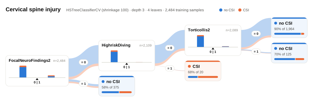
Install with pip install imodels (see here for help).
🗂️ Docs 📄 Research paper 🔗 Reference code implementation
| Model | Reference | Description |
|---|---|---|
| Rulefit rule set | 🗂️, 📄, 🔗 | Fits a sparse linear model on rules extracted from decision trees |
| Skope rule set | 🗂️, 🔗 | Extracts rules from gradient-boosted trees, deduplicates them, then linearly combines them based on their OOB precision |
| Boosted rule set | 🗂️, 📄, 🔗 | Sequentially fits a set of rules with Adaboost |
| Slipper rule set | 🗂️, 📄 | Sequentially learns a set of rules with SLIPPER |
| Bayesian rule set | 🗂️, 📄, 🔗 | Finds concise rule set with Bayesian sampling (slow) |
| Bayesian rule list | 🗂️, 📄, 🔗 | Fits compact rule list distribution with Bayesian sampling (slow) |
| Greedy rule list | 🗂️, 🔗 | Uses CART to fit a list (only a single path), rather than a tree |
| FFTree rule list | 🗂️ 🔗 | Heuristic for fitting fast and frugal rule lists |
| OneR rule list | 🗂️, 📄 | Fits rule list restricted to only one feature |
| Greedy rule tree | 🗂️, 📄, 🔗 | Greedily fits tree using CART |
| C4.5 rule tree | 🗂️, 📄, 🔗 | Greedily fits tree using C4.5 |
| Fast small tree | 🗂️,ㅤ📄 | Fast implementation of optimal tree for a given penalty per leaf |
| TAO rule tree | 🗂️, 📄 | Fits tree using alternating optimization |
| Iterative random forest | 🗂️, 📄, 🔗 | Repeatedly fit random forest, giving features with high importance a higher chance of being selected |
| Sparse integer linear model | 🗂️, 📄 | Sparse linear model with integer coefficients |
| Fast risk score | 🗂️,ㅤ📄 | Sparse integer risk score (a few features, small integer points), fit fast |
| Tree GAM | 🗂️, 📄, 🔗 | Generalized additive model fit with short boosted trees |
| GP GAM | 🗂️,ㅤ📄 | Adaptive GAM based on Gaussian processes |
| Greedy tree sums (FIGS) | 🗂️,ㅤ📄 | Sum of small trees with very few total rules (FIGS) |
| Hierarchical shrinkage wrapper | 🗂️, 📄 | Improve a decision tree, random forest, or gradient-boosting ensemble with ultra-fast, post-hoc regularization |
| RF+ (MDI+) | 🗂️, 📄 | Flexible random forest-based feature importance |
| Distillation wrapper | 🗂️ | Train a black-box model, then distill it into an interpretable model |
| AutoML wrapper | 🗂️ | Automatically fit and select an interpretable model |
| More models | ⌛ | (Coming soon!) Lightweight Rule Induction, MLRules, <Your model!> |
Demos are contained in the notebooks folder
imodels for deriving a clinical decision rule
The final form of the above models takes one of the following forms, which aim to be simultaneously simple to understand and highly predictive:
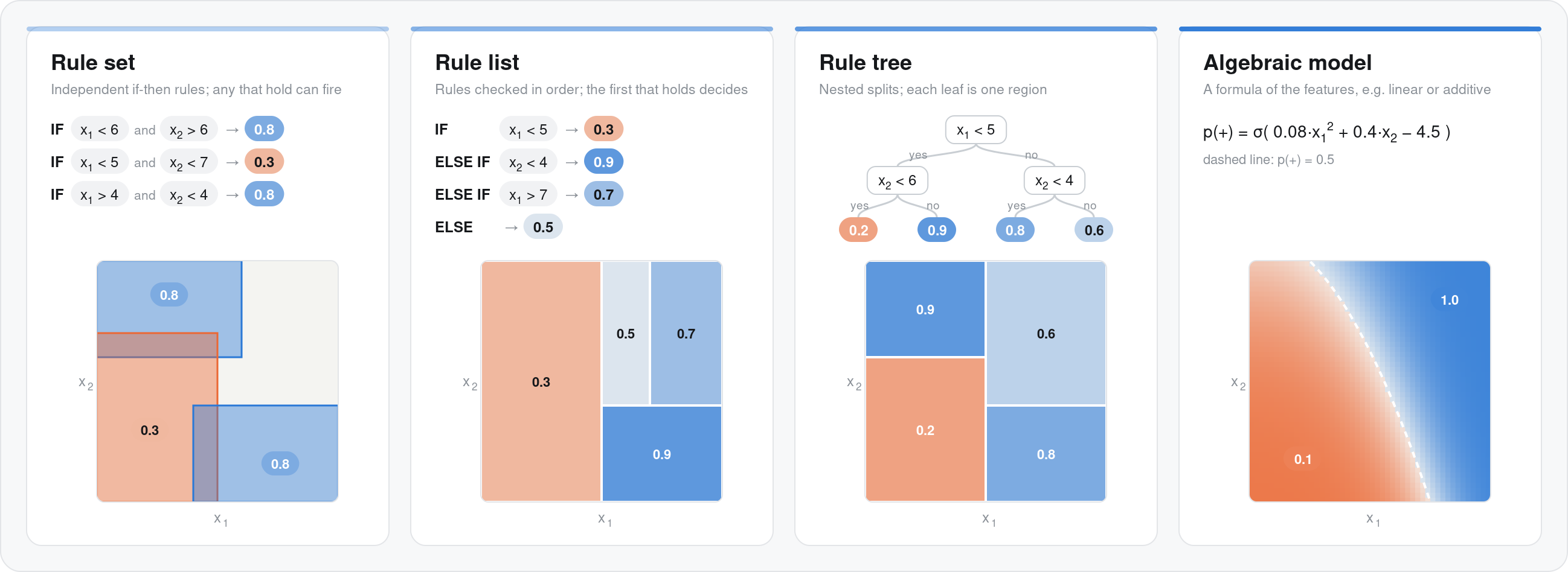
Different models support different machine-learning tasks. Current support for different models is given below (each of these models can be imported directly from imodels (e.g. from imodels import RuleFitClassifier):
All of these models follow the standard sklearn estimator API, which is checked for every model in tests/model_api_test.py: fit returns the estimator, predict returns labels drawn from classes_ (strings included), predict_proba returns an (n_samples, n_classes) matrix whose rows sum to 1, DataFrame input sets feature_names_in_,, models can be cloned and configured with get_params/set_params, and every model works inside sklearn pipelines and grid searches.
| Model | Binary classification | Regression | Notes |
|---|---|---|---|
| Rulefit rule set | RuleFitClassifier | RuleFitRegressor | |
| Skope rule set | SkopeRulesClassifier | ||
| FPSkope rule set | FPSkopeClassifier | Like Skope, but generates candidate rules with FPGrowth; requires discretized features | |
| Rulefit rule set (XGBoost) | pass tree_generator=XGBClassifier(...) to RuleFitClassifier | pass tree_generator=XGBRegressor(...) to RuleFitRegressor | Requires xgboost |
| FPLasso rule set | FPLassoClassifier | FPLassoRegressor | Lasso over rules mined with FPGrowth; requires discretized features |
| Boosted rule set | BoostedRulesClassifier | BoostedRulesRegressor | |
| SLIPPER rule set | SlipperClassifier | ||
| Bayesian rule set | BayesianRuleSetClassifier | Fails for large problems | |
| Bayesian rule list | BayesianRuleListClassifier | ||
| Greedy rule list | GreedyRuleListClassifier | ||
| OneR rule list | OneRClassifier | ||
| Greedy rule tree (CART) | GreedyTreeClassifier | GreedyTreeRegressor | |
| C4.5 rule tree | C45TreeClassifier | ||
| Optimal rule tree | FastSmallTreeClassifier | Certifiably optimal rather than greedy; needs numba | |
| CCP-pruned rule tree | DecisionTreeCCPClassifier | DecisionTreeCCPRegressor | Prunes a tree to a target complexity via cost-complexity pruning |
| TAO rule tree | TaoTreeClassifier | TaoTreeRegressor | |
| Iterative random forest | IRFClassifier | IRFRegressor | Usage and interaction stability |
| Sparse integer linear model | SLIMClassifier | SLIMRegressor | Requires extra dependencies for speed |
| Sparse integer risk score | FastRiskScoreClassifier | Binary targets; binarizes features itself; needs numba | |
| Tree GAM | TreeGAMClassifier | TreeGAMRegressor | |
| GP GAM | GPGamRegressor | GAM with pairwise interactions; nothing to tune, and deterministic | |
| Greedy tree sums (FIGS) | FIGSClassifier | FIGSRegressor | |
| Hierarchical shrinkage | HSTreeClassifierCV | HSTreeRegressorCV | Wraps any sklearn tree-based model |
| Marginal shrinkage linear model | MarginalShrinkageLinearRegressor | Linear model shrunk towards its marginal effects | |
| BART | BART | Bayesian additive regression trees (slow) | |
| Distillation | DistilledRegressor | Wraps any sklearn-compatible models | |
| AutoML model | AutoInterpretableClassifier️ | AutoInterpretableRegressor️ |
Feature scaling. Most models here work on raw features. SLIMClassifier and
SLIMRegressor are the exception: their coefficients are integers, so features
on very different scales collapse to zero when rounded. Standardize X before
fitting them (they warn if rounding has removed most of the model).
Multiclass. These classifiers handle more than two classes: FIGSClassifier,
GreedyTreeClassifier, HSTreeClassifier, TaoTreeClassifier,
BoostedRulesClassifier, SLIMClassifier, C45TreeClassifier,
DecisionTreeCCPClassifier, FastSmallTreeClassifier, IRFClassifier and the CV variants. The rule-set and rule-list models, and
FastRiskScoreClassifier, are binary-only and raise a
clear error if given a multiclass target, rather than silently treating it as
binary.
Categorical features. FIGS takes them directly — pass the column names and
it one-hot encodes them internally, remembering them for predict:
model = FIGSClassifier().fit(X, y, categorical_features=['pet', 'city'])
model.predict(X)
Other models expect numeric input, so encode categorical columns first (e.g. with
sklearn.preprocessing.OneHotEncoder, or one of the
discretizers for numeric
columns that a rule model needs binarized).
Tree-based models can be drawn with dtreeviz.
shadow_tree builds the ShadowDecTree it needs from any imodels tree model:
import dtreeviz
from imodels import FIGSClassifier, shadow_tree

model = FIGSClassifier(max_rules=6).fit(X, y)
viz = dtreeviz.trees.DTreeVizAPI(shadow_tree(model, X, y))
viz.view()
For a model made of several trees (FIGS, boosted rules), pass tree_num to pick
one. Feature and class names default to those the model was fitted with.
dtreeviz is not a dependency and is imported only when this is called.
Every rule-based model exposes its rules the same way, as a pandas DataFrame with
one row per rule, via get_rules():
from imodels import FIGSClassifier

model = FIGSClassifier(max_rules=4).fit(X_train, y_train, feature_names=feature_names)
model.get_rules()
                                               rule  prediction  tree
0                        FocalNeuroFindings2 <= 0.5       0.117     0
1                         FocalNeuroFindings2 > 0.5       0.427     0
2                             HighriskDiving <= 0.5      -0.008     1
3                              HighriskDiving > 0.5       0.550     1
4  PainNeck2 <= 0.5 and AlteredMentalStatus2 <= 0.5      -0.083     2
5   PainNeck2 <= 0.5 and AlteredMentalStatus2 > 0.5       0.048     2
6                                   PainNeck2 > 0.5       0.058     2
Two columns are always present: rule, the condition as a string, and prediction,
what that rule predicts. Models add their own columns on top — coef, support and
importance for RuleFit, tree for models made of several trees, and weight for
boosted ensembles, which combine their trees by weighted vote. Where a model is
additive, as FIGS is, prediction is that tree's contribution, so the contributions
of the matching rules sum to the model's output.
This works across rule sets, rule lists and tree-based models (RuleFit, SkopeRules,
SLIPPER, greedy and Bayesian rule lists, FIGS, CART, C4.5, TAO, boosted rules, and
hierarchical shrinkage, including the CV variants). It is also available as a
function, imodels.get_rules(model), and takes an optional feature_names argument
to rename the features. Models that aren't rule-based raise a clear error.
Tree-based models expose feature_importances_ (mean decrease in impurity), the
same measure sklearn's tree models report, so they can be compared directly.
Tree-based models also expose apply(X), which reports which leaf each sample
falls into, using the same node numbering as scikit-learn. A single tree returns
one index per sample; a model made of several trees (FIGS, boosted rules) returns
one column per tree, like RandomForest.apply.
After developing and playing with imodels, we developed a few new models to overcome limitations of existing interpretable models.
Fast Interpretable Greedy-Tree Sums (FIGS) is an algorithm for fitting concise rule-based models. Specifically, FIGS generalizes CART to simultaneously grow a flexible number of trees in a summation. The total number of splits across all the trees can be restricted by a pre-specified threshold, keeping the model interpretable. Experiments across a wide array of real-world datasets show that FIGS achieves state-of-the-art prediction performance when restricted to just a few splits (e.g. less than 20).
FastRiskScore fits a risk score: at most k conditions, each worth a few integer points, with a calibrated risk for every total. It came out of an autoresearch loop that started from FasterRisk, and adds a local search over the integer points to FasterRisk's beam search. Numeric columns are split at quantiles (n_thresholds, default 9), and the search needs numba (compiled once per machine, in about two minutes).
On 27 held-out TabArena datasets it fits about 225× faster than FasterRisk with a lower training loss, and on small problems it finds the best possible score in 49 of 50 cases (FasterRisk: 28).
GPGam fits a generalized additive model with pairwise interactions, in which every shape function is a Gaussian process over the quantile bins of its feature. Binning reduces the exact likelihood to a few sums over the data, so the likelihood alone picks the smoothness, drops irrelevant features and chooses the interactions: there is nothing to tune, fits are deterministic, and every curve comes with a posterior band.
It is the strongest interpretable model on our development suite (65 datasets) and on held-out TabArena and OpenML-CTR23 datasets.
FastSmallTree fits the decision tree that minimizes error plus a penalty per leaf over all trees on the binarized features, and certifies that no other tree scores better (the objective of GOSDT and STreeD). It came out of an autoresearch loop and compiles its branch-and-bound search with numba (about 20 seconds once per machine). regularization is the only hyperparameter.
On held-out TabArena benchmarks it matches the trees of existing optimal-tree packages while running faster, sometimes by more than 20×.
📄 Paper (ICML 2022), 🔗 Post, 📌 Citation
Hierarchical shrinkage is an extremely fast post-hoc regularization method which works on any decision tree (or tree-based ensemble, such as Random Forest). It does not modify the tree structure, and instead regularizes the tree by shrinking the prediction over each node towards the sample means of its ancestors (using a single regularization parameter). Experiments over a wide variety of datasets show that hierarchical shrinkage substantially increases the predictive performance of individual decision trees and decision-tree ensembles.
MDI+ is a novel feature importance framework, which generalizes the popular mean decrease in impurity (MDI) importance score for random forests. At its core, MDI+ expands upon a recently discovered connection between linear regression and decision trees. In doing so, MDI+ enables practitioners to (1) tailor the feature importance computation to the data/problem structure and (2) incorporate additional features or knowledge to mitigate known biases of decision trees. In both real data case studies and extensive real-data-inspired simulations, MDI+ outperforms commonly used feature importance measures (e.g., MDI, permutation-based scores, and TreeSHAP) by substantional margins.
Please cite the package if you use it in an academic work :)
@software{
	singh2021imodels,
	title        = {imodels: a python package for fitting interpretable models},
	journal      = {Journal of Open Source Software},
	publisher    = {The Open Journal},
	year         = {2021},
	author       = {Singh, Chandan and Nasseri, Keyan and Tan, Yan Shuo and Tang, Tiffany and Yu, Bin},
	volume       = {6},
	number       = {61},
	pages        = {3192},
	doi          = {10.21105/joss.03192},
	url          = {https://doi.org/10.21105/joss.03192},
}
Overall
Maintained
Code review
PyPI
Latest release
Releases this year
283 followers · starred Feb 2021
2,848 followers · starred Feb 2022
1,118 followers · starred Nov 2022
31 followers · starred Oct 2023
Interpretable ML package 🔍 for concise, transparent, and accurate predictive modeling (sklearn-compatible).
See the code
Python package for concise, transparent, and accurate predictive modeling.
All sklearn-compatible and easy to use.
Check out our new packages! Interpretability in text: imodelsX, interpretability tools for tabular data with agents: agentic-imodels
Modern machine-learning models are increasingly complex, often making them difficult to interpret. This package provides a simple interface for fitting and using state-of-the-art interpretable models, all compatible with scikit-learn. These models can often replace black-box models (e.g. random forests) with simpler models (e.g. rule lists) while improving interpretability and computational efficiency, all without sacrificing predictive accuracy! Simply import a classifier or regressor and use the fit and predict methods, same as standard scikit-learn models.
from imodels import get_clean_dataset, viz, HSTreeClassifierCV # import any imodels model here
from sklearn.model_selection import train_test_split

# prepare data (a sample clinical dataset)
X, y, feature_names = get_clean_dataset('csi_pecarn_pred')
X_train, X_test, y_train, y_test = train_test_split(
    X, y, random_state=42)

# fit the model
model = HSTreeClassifierCV(max_leaf_nodes=4)  # initialize a tree model and specify only 4 leaf nodes
model.fit(X_train, y_train, feature_names=feature_names)   # fit model
preds = model.predict(X_test) # discrete predictions: shape is (n_test, 1)
preds_proba = model.predict_proba(X_test) # predicted probabilities: shape is (n_test, n_classes)
viz.draw(model, X_train, y_train, feature_names=feature_names, class_names=["no CSI", "CSI"],
         title="Cervical spine injury", orientation="LR").save("model.svg")  # draw the model (or print(model) for text, viz.interactive(model) for interaction)
Install with pip install imodels (see here for help).
🗂️ Docs 📄 Research paper 🔗 Reference code implementation
| Model | Reference | Description |
|---|---|---|
| Rulefit rule set | 🗂️, 📄, 🔗 | Fits a sparse linear model on rules extracted from decision trees |
| Skope rule set | 🗂️, 🔗 | Extracts rules from gradient-boosted trees, deduplicates them, then linearly combines them based on their OOB precision |
| Boosted rule set | 🗂️, 📄, 🔗 | Sequentially fits a set of rules with Adaboost |
| Slipper rule set | 🗂️, 📄 | Sequentially learns a set of rules with SLIPPER |
| Bayesian rule set | 🗂️, 📄, 🔗 | Finds concise rule set with Bayesian sampling (slow) |
| Bayesian rule list | 🗂️, 📄, 🔗 | Fits compact rule list distribution with Bayesian sampling (slow) |
| Greedy rule list | 🗂️, 🔗 | Uses CART to fit a list (only a single path), rather than a tree |
| FFTree rule list | 🗂️ 🔗 | Heuristic for fitting fast and frugal rule lists |
| OneR rule list | 🗂️, 📄 | Fits rule list restricted to only one feature |
| Greedy rule tree | 🗂️, 📄, 🔗 | Greedily fits tree using CART |
| C4.5 rule tree | 🗂️, 📄, 🔗 | Greedily fits tree using C4.5 |
| Fast small tree | 🗂️,ㅤ📄 | Fast implementation of optimal tree for a given penalty per leaf |
| TAO rule tree | 🗂️, 📄 | Fits tree using alternating optimization |
| Iterative random forest | 🗂️, 📄, 🔗 | Repeatedly fit random forest, giving features with high importance a higher chance of being selected |
| Sparse integer linear model | 🗂️, 📄 | Sparse linear model with integer coefficients |
| Fast risk score | 🗂️,ㅤ📄 | Sparse integer risk score (a few features, small integer points), fit fast |
| Tree GAM | 🗂️, 📄, 🔗 | Generalized additive model fit with short boosted trees |
| GP GAM | 🗂️,ㅤ📄 | Adaptive GAM based on Gaussian processes |
| Greedy tree sums (FIGS) | 🗂️,ㅤ📄 | Sum of small trees with very few total rules (FIGS) |
| Hierarchical shrinkage wrapper | 🗂️, 📄 | Improve a decision tree, random forest, or gradient-boosting ensemble with ultra-fast, post-hoc regularization |
| RF+ (MDI+) | 🗂️, 📄 | Flexible random forest-based feature importance |
| Distillation wrapper | 🗂️ | Train a black-box model, then distill it into an interpretable model |
| AutoML wrapper | 🗂️ | Automatically fit and select an interpretable model |
| More models | ⌛ | (Coming soon!) Lightweight Rule Induction, MLRules, <Your model!> |
Demos are contained in the notebooks folder
imodels for deriving a clinical decision rule
The final form of the above models takes one of the following forms, which aim to be simultaneously simple to understand and highly predictive:
Different models support different machine-learning tasks. Current support for different models is given below (each of these models can be imported directly from imodels (e.g. from imodels import RuleFitClassifier):
All of these models follow the standard sklearn estimator API, which is checked for every model in tests/model_api_test.py: fit returns the estimator, predict returns labels drawn from classes_ (strings included), predict_proba returns an (n_samples, n_classes) matrix whose rows sum to 1, DataFrame input sets feature_names_in_,, models can be cloned and configured with get_params/set_params, and every model works inside sklearn pipelines and grid searches.
| Model | Binary classification | Regression | Notes |
|---|---|---|---|
| Rulefit rule set | RuleFitClassifier | RuleFitRegressor | |
| Skope rule set | SkopeRulesClassifier | ||
| FPSkope rule set | FPSkopeClassifier | Like Skope, but generates candidate rules with FPGrowth; requires discretized features | |
| Rulefit rule set (XGBoost) | pass tree_generator=XGBClassifier(...) to RuleFitClassifier | pass tree_generator=XGBRegressor(...) to RuleFitRegressor | Requires xgboost |
| FPLasso rule set | FPLassoClassifier | FPLassoRegressor | Lasso over rules mined with FPGrowth; requires discretized features |
| Boosted rule set | BoostedRulesClassifier | BoostedRulesRegressor | |
| SLIPPER rule set | SlipperClassifier | ||
| Bayesian rule set | BayesianRuleSetClassifier | Fails for large problems | |
| Bayesian rule list | BayesianRuleListClassifier | ||
| Greedy rule list | GreedyRuleListClassifier | ||
| OneR rule list | OneRClassifier | ||
| Greedy rule tree (CART) | GreedyTreeClassifier | GreedyTreeRegressor | |
| C4.5 rule tree | C45TreeClassifier | ||
| Optimal rule tree | FastSmallTreeClassifier | Certifiably optimal rather than greedy; needs numba | |
| CCP-pruned rule tree | DecisionTreeCCPClassifier | DecisionTreeCCPRegressor | Prunes a tree to a target complexity via cost-complexity pruning |
| TAO rule tree | TaoTreeClassifier | TaoTreeRegressor | |
| Iterative random forest | IRFClassifier | IRFRegressor | Usage and interaction stability |
| Sparse integer linear model | SLIMClassifier | SLIMRegressor | Requires extra dependencies for speed |
| Sparse integer risk score | FastRiskScoreClassifier | Binary targets; binarizes features itself; needs numba | |
| Tree GAM | TreeGAMClassifier | TreeGAMRegressor | |
| GP GAM | GPGamRegressor | GAM with pairwise interactions; nothing to tune, and deterministic | |
| Greedy tree sums (FIGS) | FIGSClassifier | FIGSRegressor | |
| Hierarchical shrinkage | HSTreeClassifierCV | HSTreeRegressorCV | Wraps any sklearn tree-based model |
| Marginal shrinkage linear model | MarginalShrinkageLinearRegressor | Linear model shrunk towards its marginal effects | |
| BART | BART | Bayesian additive regression trees (slow) | |
| Distillation | DistilledRegressor | Wraps any sklearn-compatible models | |
| AutoML model | AutoInterpretableClassifier️ | AutoInterpretableRegressor️ |
Feature scaling. Most models here work on raw features. SLIMClassifier and
SLIMRegressor are the exception: their coefficients are integers, so features
on very different scales collapse to zero when rounded. Standardize X before
fitting them (they warn if rounding has removed most of the model).
Multiclass. These classifiers handle more than two classes: FIGSClassifier,
GreedyTreeClassifier, HSTreeClassifier, TaoTreeClassifier,
BoostedRulesClassifier, SLIMClassifier, C45TreeClassifier,
DecisionTreeCCPClassifier, FastSmallTreeClassifier, IRFClassifier and the CV variants. The rule-set and rule-list models, and
FastRiskScoreClassifier, are binary-only and raise a
clear error if given a multiclass target, rather than silently treating it as
binary.
Categorical features. FIGS takes them directly — pass the column names and
it one-hot encodes them internally, remembering them for predict:
model = FIGSClassifier().fit(X, y, categorical_features=['pet', 'city'])
model.predict(X)
Other models expect numeric input, so encode categorical columns first (e.g. with
sklearn.preprocessing.OneHotEncoder, or one of the
discretizers for numeric
columns that a rule model needs binarized).
Tree-based models can be drawn with dtreeviz.
shadow_tree builds the ShadowDecTree it needs from any imodels tree model:
import dtreeviz
from imodels import FIGSClassifier, shadow_tree

model = FIGSClassifier(max_rules=6).fit(X, y)
viz = dtreeviz.trees.DTreeVizAPI(shadow_tree(model, X, y))
viz.view()
For a model made of several trees (FIGS, boosted rules), pass tree_num to pick
one. Feature and class names default to those the model was fitted with.
dtreeviz is not a dependency and is imported only when this is called.
Every rule-based model exposes its rules the same way, as a pandas DataFrame with
one row per rule, via get_rules():
from imodels import FIGSClassifier

model = FIGSClassifier(max_rules=4).fit(X_train, y_train, feature_names=feature_names)
model.get_rules()
                                               rule  prediction  tree
0                        FocalNeuroFindings2 <= 0.5       0.117     0
1                         FocalNeuroFindings2 > 0.5       0.427     0
2                             HighriskDiving <= 0.5      -0.008     1
3                              HighriskDiving > 0.5       0.550     1
4  PainNeck2 <= 0.5 and AlteredMentalStatus2 <= 0.5      -0.083     2
5   PainNeck2 <= 0.5 and AlteredMentalStatus2 > 0.5       0.048     2
6                                   PainNeck2 > 0.5       0.058     2
Two columns are always present: rule, the condition as a string, and prediction,
what that rule predicts. Models add their own columns on top — coef, support and
importance for RuleFit, tree for models made of several trees, and weight for
boosted ensembles, which combine their trees by weighted vote. Where a model is
additive, as FIGS is, prediction is that tree's contribution, so the contributions
of the matching rules sum to the model's output.
This works across rule sets, rule lists and tree-based models (RuleFit, SkopeRules,
SLIPPER, greedy and Bayesian rule lists, FIGS, CART, C4.5, TAO, boosted rules, and
hierarchical shrinkage, including the CV variants). It is also available as a
function, imodels.get_rules(model), and takes an optional feature_names argument
to rename the features. Models that aren't rule-based raise a clear error.
Tree-based models expose feature_importances_ (mean decrease in impurity), the
same measure sklearn's tree models report, so they can be compared directly.
Tree-based models also expose apply(X), which reports which leaf each sample
falls into, using the same node numbering as scikit-learn. A single tree returns
one index per sample; a model made of several trees (FIGS, boosted rules) returns
one column per tree, like RandomForest.apply.
After developing and playing with imodels, we developed a few new models to overcome limitations of existing interpretable models.
Fast Interpretable Greedy-Tree Sums (FIGS) is an algorithm for fitting concise rule-based models. Specifically, FIGS generalizes CART to simultaneously grow a flexible number of trees in a summation. The total number of splits across all the trees can be restricted by a pre-specified threshold, keeping the model interpretable. Experiments across a wide array of real-world datasets show that FIGS achieves state-of-the-art prediction performance when restricted to just a few splits (e.g. less than 20).
FastRiskScore fits a risk score: at most k conditions, each worth a few integer points, with a calibrated risk for every total. It came out of an autoresearch loop that started from FasterRisk, and adds a local search over the integer points to FasterRisk's beam search. Numeric columns are split at quantiles (n_thresholds, default 9), and the search needs numba (compiled once per machine, in about two minutes).
On 27 held-out TabArena datasets it fits about 225× faster than FasterRisk with a lower training loss, and on small problems it finds the best possible score in 49 of 50 cases (FasterRisk: 28).
GPGam fits a generalized additive model with pairwise interactions, in which every shape function is a Gaussian process over the quantile bins of its feature. Binning reduces the exact likelihood to a few sums over the data, so the likelihood alone picks the smoothness, drops irrelevant features and chooses the interactions: there is nothing to tune, fits are deterministic, and every curve comes with a posterior band.
It is the strongest interpretable model on our development suite (65 datasets) and on held-out TabArena and OpenML-CTR23 datasets.
FastSmallTree fits the decision tree that minimizes error plus a penalty per leaf over all trees on the binarized features, and certifies that no other tree scores better (the objective of GOSDT and STreeD). It came out of an autoresearch loop and compiles its branch-and-bound search with numba (about 20 seconds once per machine). regularization is the only hyperparameter.
On held-out TabArena benchmarks it matches the trees of existing optimal-tree packages while running faster, sometimes by more than 20×.
📄 Paper (ICML 2022), 🔗 Post, 📌 Citation
Hierarchical shrinkage is an extremely fast post-hoc regularization method which works on any decision tree (or tree-based ensemble, such as Random Forest). It does not modify the tree structure, and instead regularizes the tree by shrinking the prediction over each node towards the sample means of its ancestors (using a single regularization parameter). Experiments over a wide variety of datasets show that hierarchical shrinkage substantially increases the predictive performance of individual decision trees and decision-tree ensembles.
MDI+ is a novel feature importance framework, which generalizes the popular mean decrease in impurity (MDI) importance score for random forests. At its core, MDI+ expands upon a recently discovered connection between linear regression and decision trees. In doing so, MDI+ enables practitioners to (1) tailor the feature importance computation to the data/problem structure and (2) incorporate additional features or knowledge to mitigate known biases of decision trees. In both real data case studies and extensive real-data-inspired simulations, MDI+ outperforms commonly used feature importance measures (e.g., MDI, permutation-based scores, and TreeSHAP) by substantional margins.
Please cite the package if you use it in an academic work :)
@software{
	singh2021imodels,
	title        = {imodels: a python package for fitting interpretable models},
	journal      = {Journal of Open Source Software},
	publisher    = {The Open Journal},
	year         = {2021},
	author       = {Singh, Chandan and Nasseri, Keyan and Tan, Yan Shuo and Tang, Tiffany and Yu, Bin},
	volume       = {6},
	number       = {61},
	pages        = {3192},
	doi          = {10.21105/joss.03192},
	url          = {https://doi.org/10.21105/joss.03192},
}
Overall
Maintained
Code review
PyPI
Latest release
Releases this year
283 followers · starred Feb 2021
2,848 followers · starred Feb 2022
1,118 followers · starred Nov 2022
31 followers · starred Oct 2023