The well-known Quicksort is a O(n log n) algorithm that uses O(n) partitioning to sort data. Such partitioning schemes are easily done in-place (O(1) extra space) but are not stable, or do not preserve the order of equal elements. Stable Quicksorts can also be done in O(n log n) time, but they use an extra O(n) space for stable partitioning and are no longer in-place.
Logsort is a novel practical O(n log n) quicksort that is both in-place and stable. The algorithm stably partitions data in O(n) time using O(log n) space, hence the name, which many already consider to be in-place despite not being the optimal O(1). Unlike well-known in-place stable sorts which are O(n log² n), such as std::stable_sort, Logsort is asymptotically optimal.
To see Logsort's practical performance, jump to Results.
[!NOTE] Usage: define
VARelement type andCMPcomparison function.
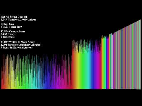
(Youtube) Logsort visualized on N = 2049 with 9 extra space allocated.
O(n log n) in-place stable sorting is hard to achieve for sorting algorithms. Bubble Sort and Insertion Sort are stable and in-place but suboptimal. Efficient sorts, such as Quicksort and Heapsort, are in-place and O(n log n) but unstable.
One class of sorting algorithms that achieve both in-place, stability, and O(n log n) time is Block Sort (a.k.a. Block Merge Sorts), such as Wikisort and Grailsort, which are in-place merge sorts. However, they are incredibly complicated and hard to implement. In addition, in-place stable partitioning is a rather obscure problem in sorting. Katajainen & Pasanen 1992 describes an O(1) space O(n) time partitioning algorithm, but it's only of theoretical interest and not practical.
Logsort is a new sorting algorithm that aims to provide a simple and practical O(n log n) in-place stable sort implementation like alternatives such as Block Sort. The algorithm uses a novel O(n) in-place stable partitioning algorithm different than Katajainen & Pasanen 1992 and borrows ideas from Aeos Quicksort (stable quicksort with O(sqrt n) size blocking). By sorting recursively using this partition, we get an O(n log n) sorting algorithm.
Partitioning is analogous to sorting an array of 0's and 1's, where elements smaller than the pivot are 0 and elements larger are 1. (Munro et al. 1990) Logsort sorts 0's and 1's stably in O(n) time and O(log n) space via its partition.
In brief, Logsort groups 0's and 1's elements into blocks of size O(log n) using its available space. By swapping elements among the 0 and 1 blocks, each block is assigned a unique index with O(log n) bits. An LL block swap partition is performed on the blocks which preserves the order of one partition but not the other. Using the assigned indices from earlier, the order of the blocks in the scrambled partition are restored. Lastly, the leftover 0's not divisible by the block length are shifted into place, and the Logsort partition is completed in O(n) time and O(log n) space.
The four phases of the partition algorithm in more detail along with proofs:
The entire partition is implemented in about 100 lines of C code: logPartition.c
Given an unordered list of 0's and 1's, we group them into blocks of a fixed size where each block contains either only 0's or 1's. Given two buckets of B extra space, one can easily group blocks of size B (Katajainen & Pasanen 1992):
Grouping blocks of size 2:

        ↓ move to ones bucket
array: [1, 0, 1, 1, 0, 0, 1, 1]
zeros: [ ,  ]
 ones: [ ,  ]

           ↓ move to zeros bucket
array: [ , 0, 1, 1, 0, 0, 1, 1]
zeros: [ ,  ]
 ones: [1,  ]

              ↓ move to ones bucket
array: [ ,  , 1, 1, 0, 0, 1, 1]
zeros: [0,  ]
 ones: [1,  ]

array: [ ,  ,  , 1, 0, 0, 1, 1]
zeros: [0,  ]
 ones: [1, 1] ← ones bucket full: output back into array

        ↓  ↓ first block created: continue looping
array: [1, 1,  , 1, 0, 0, 1, 1]
zeros: [0,  ]
 ones: [ ,  ]
It's almost guaranteed we end up with partially filled buckets at the end of this phase. In that case, we output the 0 elements followed by the 1's at the end of the array.
                          ↓ output zeros
array: [1, 1, 0, 0, 1, 1,  ,  ]
zeros: [0,  ]
 ones: [1,  ]

                             ↓ output ones
array: [1, 1, 0, 0, 1, 1, 0,  ]
zeros: [ ,  ]
 ones: [1,  ]


array: [1, 1, 0, 0, 1, 1, 0, 1]

       ┌──── blocks ────┐ ↓ leftover zeros
       [1, 1][0, 0][1, 1][0][1]
At the end of the phase, we are left with some leftover zeros that don't make a complete block. We handle them in the very last step of the partition.
Logsort's O(log n) space usage comes from grouping blocks of size O(log n), and this will be important in the encoding phase. In the actual implementation, a space optimization from Aeos Quicksort is used which only needs one bucket instead of two. (Anonymous0726 2021) Like Wikisort and Grailsort, Logsort's external buffer size can be configured, given it's at least Ω(log n).
Since each element is moved a constant number of times, once to the bucket and once back to the array, the grouping phase is O(n) regardless of block size but requires O(block size) extra space.
0's and 1's can also be concatenated to make binary numbers, so we can encode numbers in blocks by swapping elements between 0 blocks and 1 blocks. Decoding a number in a block requires a scan of the block which costs O(log n) comparisons. Since Logsort's blocks are O(log n) in size, there are enough bits to assign a unique index to each block.
There are at most O(n/log n) encodable blocks which require log(n/log n) = O(log n) bits to represent a number range from 0 to O(n/log n).
Encode decimal number 13 = 0b1101:

[0, 0, 0, 0, 0] [1, 1, 1, 1, 1]
 ↑  ↑     ↑      ↑  ↑     ↑
 1  2     3      1  2     3  ← swap the following

┌─── 13 ───┐    ┌── ~13 ───┐
[1, 1, 0, 1, 0] [0, 0, 1, 0, 1] ← the pair of blocks are now encoded with 13
             ↑               ↑
             last bit reserved to determine 0 or 1 block
Using this technique, pairs of 0 and 1 block are encoded with a unique index during the encoding phase. We maintain two iterators: one for 0 blocks and 1 blocks respectively:
Encode blocks:

 (0)  (0)
[ 0 ][ 1 ][ 1 ][ 1 ][ 0 ][ 1 ][ 0 ][ 1 ]
└───┘└───┘ encode 0

 (0)  (0)  (1)       (1)
[ 0 ][ 1 ][ 1 ][ 1 ][ 0 ][ 1 ][ 0 ][ 1 ]
          └───┘     └───┘ encode 1

 (0)  (0)  (1)  (2)  (1)       (2)
[ 0 ][ 1 ][ 1 ][ 1 ][ 0 ][ 1 ][ 0 ][ 1 ]
               └───┘          └───┘ encode 2 and finish
In this example, there were fewer 0 blocks, so all 0 blocks get encoded leaving some 1 blocks untouched. These leftover blocks will be handled in the swapping phase.
Encoding an index costs O(log n) swaps. Since each block is size O(log n), there are O(n/log n) blocks, so this phase is O(n/log n) * O(log n) = O(n).
Once the blocks are encoded, we swap the blocks belonging to the larger partition. In our example, there are more 1 blocks than 0 blocks so we scan the blocks' reserved bit and swap the 1 blocks to the right into their correct place:
Swap blocks:

 (0)   (0)   (1)   (2)   (1)         (2)
[ 0a ][ 1a ][ 1b ][ 1c ][ 0b ][ 1d ][ 0c ][ 1e ]
                              └────┘└────┘ block swap

 (0)   (0)   (1)   (2)   (1)   (2)
[ 0a ][ 1a ][ 1b ][ 1c ][ 0b ][ 0c ][ 1d ][ 1e ]
                  └────┘      └────┘ block swap

 (0)   (0)   (1)   (2)   (1)   (2)
[ 0a ][ 1a ][ 1b ][ 0c ][ 0b ][ 1c ][ 1d ][ 1e ]
            └────┘      └────┘ block swap

 (0)   (0)   (1)   (2)   (1)   (2)
[ 0a ][ 1a ][ 0b ][ 0c ][ 1b ][ 1c ][ 1d ][ 1e ]
      └────┘      └────┘ block swap

 (0)   (2)   (1)   (0)   (1)   (2)
[ 0a ][ 0c ][ 0b ][ 1a ][ 1b ][ 1c ][ 1d ][ 1e ]
                         (finished block swapping)
Swapping blocks in this fashion preserves the order of the 1 blocks. If there were more 0 blocks, we would swap them to the left. In this example, after swapping, the 1's partition is stably ordered. However, the order of the 0 blocks is now scrambled. Using the encoded indices in the 0 blocks, we can reorder them stably in the sorting phase.
Each block in the phase is swapped once. Since each block swap costs O(log n) swaps and there are at most O(n/log n) blocks swapped, the swapping phase is O(n/log n) * O(log n) = O(n).
Reordering the scrambled blocks is quite easy: simply iterate across the blocks. If the current block's index is not equal to the iterator, block swap the current block to the read index. Repeat this step until the current block's index matches the iterator and move on to the next block.
Sort blocks:

 (0)←  (2)   (1)   (0)   (1)   (2)
[ 0a ][ 0c ][ 0b ][ 1a ][ 1b ][ 1c ][ 1d ][ 1e ]
└────┘ 0th block == 0 ? -> Yes: go to next block

 (0)   (2)←  (1)   (0)   (1)   (2)
[ 0a ][ 0c ][ 0b ][ 1a ][ 1b ][ 1c ][ 1d ][ 1e ]
      └────┘ 1st block == 2 ? -> No: swap with 2nd block

 (0)   (1)   (2)   (0)   (1)   (2)
[ 0a ][ 0b ][ 0c ][ 1a ][ 1b ][ 1c ][ 1d ][ 1e ]
      └────┘└────┘

 (0)   (1)←  (2)   (0)   (1)   (2)
[ 0a ][ 0b ][ 0c ][ 1a ][ 1b ][ 1c ][ 1d ][ 1e ]
      └────┘ 1st block == 1 ? -> Yes: go to next block

 (0)   (1)   (2)←  (0)   (1)   (2)
[ 0a ][ 0b ][ 0c ][ 1a ][ 1b ][ 1c ][ 1d ][ 1e ]
            └────┘ 2nd block == 2 ? -> Yes: finish
In pseudocode:
for each index from 0 to blocks.count - 1:
	current = blocks[index].decode()
	while current != index:
		block swap blocks[current] and blocks[index]
		current = blocks[index].decode()
It's worth noting in our example we sorted the blocks belonging to the 0 partition. However, recall that the encoding of 1 blocks is the bit flip of 0 blocks, so we would need to bit flip the results of the decoding beforehand in the case of sorting 1 blocks.
Each time a block is swapped, it ends up in its final destination, therefore a block is swapped at most once. The blocks are also decoded at most twice: once per block swap and once per iterated block.
Combined, the operations on a block are O(log n). Since there are at most O(n/log n) scrambled blocks, the sorting phase is O(n/log n) * O(log n) = O(n).
After the sorting phase, the blocks are now partitioned stably in O(n) time. However, some elements between blocks are still swapped from the encoding phase, and we want to restore the original states of the blocks. Since both 0 blocks and 1 blocks are in order, we can easily reaccess the original encoded block pairs along with their indices in ascending order. We then can "uncode" them by applying the encode algorithm again with the same index. After iterating and uncoding the block pairs, we complete the partition on the blocks.
Uncode blocks:

 (0)   (1)   (2)   (0)   (1)   (2)
[ 0a ][ 0b ][ 0c ][ 1a ][ 1b ][ 1c ][ 1d ][ 1e ]
└────┘            └────┘ uncode 0 (encode 0)

       (1)   (2)         (1)   (2)
[ 0a ][ 0b ][ 0c ][ 1a ][ 1b ][ 1c ][ 1d ][ 1e ]
      └────┘            └────┘ uncode 1 (encode 1)

             (2)               (2)
[ 0a ][ 0b ][ 0c ][ 1a ][ 1b ][ 1c ][ 1d ][ 1e ]
            └────┘            └────┘ uncode 2 (encode 2)

[ 0a ][ 0b ][ 0c ][ 1a ][ 1b ][ 1c ][ 1d ][ 1e ]
[       0        ][             1              ]

blocks and underlying elements partitioned stably!
We are not done yet and still have a leftover chunk of 0's that did not make a complete block from the grouping phase. Simply copy the 0 leftovers, shift the 1's partition to the right, and copy the leftovers back:
Clean up:

[0 0 0 0 0][1 1 1 1 1 1 1 1 1 1 1 1][0 0 0][1 1 1]
                                    └─────┘ copy out

[0 0 0 0 0][1 1 1 1 1 1 1 1 1 1 1 1]       [1 1 1]
           └───────────────────────┘ shift --->

[0 0 0 0 0]       [1 1 1 1 1 1 1 1 1 1 1 1][1 1 1]
           └─────┘ copy in

[0 0 0 0 0][0 0 0][1 1 1 1 1 1 1 1 1 1 1 1][1 1 1]
└─────── 0 ──────┘└────────────── 1 ─────────────┘

partition complete!
Finally, we've stably partitioned the list in O(n) time and O(log n) space.
There are O(n/log n) pairs of blocks that need to be uncoded. Since each uncoding operation is O(log n), it costs O(n/log n) * O(log n) = O(n) operations.
Copying the leftovers and shifting the 1's partition is O(n) + O(log n) = O(n).
An O(n log n) in-place stable sort in theory sounds great, but how does it compare against existing sorts? In the following benchmarks, we test Logsort's practicality against four other stable sorting algorithms:
All sorts are compiled with gcc -O3 using GCC 11.4.0 and ran on Ubuntu 22.04 using WSL. The algorithms sort a random linear distribution of 32-bit integers containing N unique, √N unique, and 4 unique values respectively. The average time among 100 trials is recorded.


| Sort | List Size | Data Type | Best Time (µs) | Avg. Time (µs) | Trials | Distribution |
|---|---|---|---|---|---|---|
| Blitsort (512) | 16384 | 4 bytes | 71 | 84 | 100 | 4 unique |
| Sqrtsort (√N) | 16384 | 4 bytes | 482 | 509 | 100 | 4 unique |
| Octosort (512) | 16384 | 4 bytes | 437 | 463 | 100 | 4 unique |
| Grailsort (512) | 16384 | 4 bytes | 855 | 923 | 100 | 4 unique |
| Logsort (512) | 16384 | 4 bytes | 107 | 119 | 100 | 4 unique |
| Sort | List Size | Data Type | Best Time (µs) | Avg. Time (µs) | Trials | Distribution |
|---|---|---|---|---|---|---|
| Blitsort (512) | 16384 | 4 bytes | 211 | 227 | 100 | 128 unique |
| Sqrtsort (√N) | 16384 | 4 bytes | 764 | 791 | 100 | 128 unique |
| Octosort (512) | 16384 | 4 bytes | 844 | 872 | 100 | 128 unique |
| Grailsort (512) | 16384 | 4 bytes | 1533 | 1590 | 100 | 128 unique |
| Logsort (512) | 16384 | 4 bytes | 375 | 397 | 100 | 128 unique |
| Sort | List Size | Data Type | Best Time (µs) | Avg. Time (µs) | Trials | Distribution |
|---|---|---|---|---|---|---|
| Blitsort (512) | 16384 | 4 bytes | 416 | 435 | 100 | 16384 unique |
| Sqrtsort (√N) | 16384 | 4 bytes | 947 | 972 | 100 | 16384 unique |
| Octosort (512) | 16384 | 4 bytes | 989 | 1012 | 100 | 16384 unique |
| Grailsort (512) | 16384 | 4 bytes | 1036 | 1064 | 100 | 16384 unique |
| Logsort (512) | 16384 | 4 bytes | 402 | 424 | 100 | 16384 unique |
| Sort | List Size | Data Type | Best Time (µs) | Avg. Time (µs) | Trials | Distribution |
|---|---|---|---|---|---|---|
| Blitsort (512) | 1048576 | 4 bytes | 5171 | 5964 | 100 | 4 unique |
| Sqrtsort (√N) | 1048576 | 4 bytes | 37006 | 38549 | 100 | 4 unique |
| Octosort (512) | 1048576 | 4 bytes | 30248 | 32028 | 100 | 4 unique |
| Grailsort (512) | 1048576 | 4 bytes | 56563 | 58549 | 100 | 4 unique |
| Logsort (512) | 1048576 | 4 bytes | 7098 | 7527 | 100 | 4 unique |
| Sort | List Size | Data Type | Best Time (µs) | Avg. Time (µs) | Trials | Distribution |
|---|---|---|---|---|---|---|
| Blitsort (512) | 1048576 | 4 bytes | 20459 | 20896 | 100 | 1024 unique |
| Sqrtsort (√N) | 1048576 | 4 bytes | 66212 | 68995 | 100 | 1024 unique |
| Octosort (512) | 1048576 | 4 bytes | 75614 | 78219 | 100 | 1024 unique |
| Grailsort (512) | 1048576 | 4 bytes | 129576 | 133018 | 100 | 1024 unique |
| Logsort (512) | 1048576 | 4 bytes | 22834 | 23245 | 100 | 1024 unique |
| Sort | List Size | Data Type | Best Time (µs) | Avg. Time (µs) | Trials | Distribution |
|---|---|---|---|---|---|---|
| Blitsort (512) | 1048576 | 4 bytes | 37693 | 39161 | 100 | 1048576 unique |
| Sqrtsort (√N) | 1048576 | 4 bytes | 87581 | 90788 | 100 | 1048576 unique |
| Octosort (512) | 1048576 | 4 bytes | 96464 | 99214 | 100 | 1048576 unique |
| Grailsort (512) | 1048576 | 4 bytes | 92196 | 95436 | 100 | 1048576 unique |
| Logsort (512) | 1048576 | 4 bytes | 37343 | 38983 | 100 | 1048576 unique |
| Sort | List Size | Data Type | Best Time (µs) | Avg. Time (µs) | Trials | Distribution |
|---|---|---|---|---|---|---|
| Blitsort (512) | 16777216 | 4 bytes | 431614 | 462105 | 100 | 4 unique |
| Sqrtsort (√N) | 16777216 | 4 bytes | 885925 | 904531 | 100 | 4 unique |
| Octosort (512) | 16777216 | 4 bytes | 657904 | 671961 | 100 | 4 unique |
| Grailsort (512) | 16777216 | 4 bytes | 1059679 | 1126016 | 100 | 4 unique |
| Logsort (512) | 16777216 | 4 bytes | 149899 | 161879 | 100 | 4 unique |
| Sort | List Size | Data Type | Best Time (µs) | Avg. Time (µs) | Trials | Distribution |
|---|---|---|---|---|---|---|
| Blitsort (512) | 16777216 | 4 bytes | 854276 | 860791 | 100 | 4096 unique |
| Sqrtsort (√N) | 16777216 | 4 bytes | 1463341 | 1499482 | 100 | 4096 unique |
| Octosort (512) | 16777216 | 4 bytes | 1682796 | 1727569 | 100 | 4096 unique |
| Grailsort (512) | 16777216 | 4 bytes | 2744438 | 2954750 | 100 | 4096 unique |
| Logsort (512) | 16777216 | 4 bytes | 484517 | 490591 | 100 | 4096 unique |
| Sort | List Size | Data Type | Best Time (µs) | Avg. Time (µs) | Trials | Distribution |
|---|---|---|---|---|---|---|
| Blitsort (512) | 16777216 | 4 bytes | 1021487 | 1030391 | 100 | 16777216 unique |
| Sqrtsort (√N) | 16777216 | 4 bytes | 1873933 | 1988718 | 100 | 16777216 unique |
| Octosort (512) | 16777216 | 4 bytes | 2123259 | 2267619 | 100 | 16777216 unique |
| Grailsort (512) | 16777216 | 4 bytes | 1965213 | 2043090 | 100 | 16777216 unique |
| Logsort (512) | 16777216 | 4 bytes | 812568 | 851833 | 100 | 16777216 unique |
Grailsort, Octosort, and Sqrtsort used branched comparisons in merging. Logsort was optimized with branchless comparisons similar to Fluxsort which greatly improved its performance with a 40% increase in speed! The explanation of this speed boost seems to be similar in mechanism to that of Block Quicksort (Edelkamp & Weiss 2016). Since Logsort is a stable quicksort by nature, branchless comparisons were easier to implement contrary to a Block Merge Sort. To further increase the performance as well as simplify the pivot selection, Piposort was also used for small arrays.
Unlike Block Merge Sorts, Logsort relies on its bit encoding to store information rather than distinct values. This avoids any overhead in a key collection algorithm; we see this happening with Grailsort spending O(n log n) comparisons finding √N uniques.
Being a stable quicksort, Logsort naturally performs well on data with few uniques boasting a O(n log u) complexity. However, for smaller array sizes, Octosort and Blitsort beat Logsort on a data size of 16M with 4 uniques despite having a complexity of O(n log n log u). This is likely due to Logsort's poorer access patterns and overhead compared to simple merges with rotations.
Logsort's main rival, Blitsort, is an optimized Rotate Merge/Quick Sort which uses rotations to merge/partition but has a suboptimal O(n log² n) complexity. Despite this, Rotate Merge is known to beat the optimal Block Merge owing to its simplicity, good locality, and low overhead.
In the benchmarks, Logsort remained competitive with Blitsort on 2^14 to 2^20 integers and even beat Blitsort on 2^24 integers and beyond with its superior time complexity. Unlike Blitsort, however, Logsort is not optimized to be an adaptive sort, and this comparison is only on random data. A hybrid between a rotate partition and blocked partition is also a good idea, but such an optimization is left to the reader. To keep the codebase as simple as possible, there is no fallback algorithm when choosing a bad pivot, so it is highly advised to include one when using this algorithm in a practical setting.
With further improvements, it's likely that stable O(n log n) in-place sorting has practical application outside of theory. It's worth noting that Logsort's application is quite galactic, only seeing noticeable benefits on lengths in the tens of millions. However, despite Logsort's simplicity compared to Block Merge Sorts, these algorithms remain fairly complicated compared to their unstable counterparts.
The author would like to thank members of the Discord server "The Studio" (https://discord.gg/thestudio) particularly:
366 followers · starred Sep 2023
131 followers · starred Jan 2026
The well-known Quicksort is a O(n log n) algorithm that uses O(n) partitioning to sort data. Such partitioning schemes are easily done in-place (O(1) extra space) but are not stable, or do not preserve the order of equal elements. Stable Quicksorts can also be done in O(n log n) time, but they use an extra O(n) space for stable partitioning and are no longer in-place.
Logsort is a novel practical O(n log n) quicksort that is both in-place and stable. The algorithm stably partitions data in O(n) time using O(log n) space, hence the name, which many already consider to be in-place despite not being the optimal O(1). Unlike well-known in-place stable sorts which are O(n log² n), such as std::stable_sort, Logsort is asymptotically optimal.
To see Logsort's practical performance, jump to Results.
[!NOTE] Usage: define
VARelement type andCMPcomparison function.
(Youtube) Logsort visualized on N = 2049 with 9 extra space allocated.
O(n log n) in-place stable sorting is hard to achieve for sorting algorithms. Bubble Sort and Insertion Sort are stable and in-place but suboptimal. Efficient sorts, such as Quicksort and Heapsort, are in-place and O(n log n) but unstable.
One class of sorting algorithms that achieve both in-place, stability, and O(n log n) time is Block Sort (a.k.a. Block Merge Sorts), such as Wikisort and Grailsort, which are in-place merge sorts. However, they are incredibly complicated and hard to implement. In addition, in-place stable partitioning is a rather obscure problem in sorting. Katajainen & Pasanen 1992 describes an O(1) space O(n) time partitioning algorithm, but it's only of theoretical interest and not practical.
Logsort is a new sorting algorithm that aims to provide a simple and practical O(n log n) in-place stable sort implementation like alternatives such as Block Sort. The algorithm uses a novel O(n) in-place stable partitioning algorithm different than Katajainen & Pasanen 1992 and borrows ideas from Aeos Quicksort (stable quicksort with O(sqrt n) size blocking). By sorting recursively using this partition, we get an O(n log n) sorting algorithm.
Partitioning is analogous to sorting an array of 0's and 1's, where elements smaller than the pivot are 0 and elements larger are 1. (Munro et al. 1990) Logsort sorts 0's and 1's stably in O(n) time and O(log n) space via its partition.
In brief, Logsort groups 0's and 1's elements into blocks of size O(log n) using its available space. By swapping elements among the 0 and 1 blocks, each block is assigned a unique index with O(log n) bits. An LL block swap partition is performed on the blocks which preserves the order of one partition but not the other. Using the assigned indices from earlier, the order of the blocks in the scrambled partition are restored. Lastly, the leftover 0's not divisible by the block length are shifted into place, and the Logsort partition is completed in O(n) time and O(log n) space.
The four phases of the partition algorithm in more detail along with proofs:
The entire partition is implemented in about 100 lines of C code: logPartition.c
Given an unordered list of 0's and 1's, we group them into blocks of a fixed size where each block contains either only 0's or 1's. Given two buckets of B extra space, one can easily group blocks of size B (Katajainen & Pasanen 1992):
Grouping blocks of size 2:

        ↓ move to ones bucket
array: [1, 0, 1, 1, 0, 0, 1, 1]
zeros: [ ,  ]
 ones: [ ,  ]

           ↓ move to zeros bucket
array: [ , 0, 1, 1, 0, 0, 1, 1]
zeros: [ ,  ]
 ones: [1,  ]

              ↓ move to ones bucket
array: [ ,  , 1, 1, 0, 0, 1, 1]
zeros: [0,  ]
 ones: [1,  ]

array: [ ,  ,  , 1, 0, 0, 1, 1]
zeros: [0,  ]
 ones: [1, 1] ← ones bucket full: output back into array

        ↓  ↓ first block created: continue looping
array: [1, 1,  , 1, 0, 0, 1, 1]
zeros: [0,  ]
 ones: [ ,  ]
It's almost guaranteed we end up with partially filled buckets at the end of this phase. In that case, we output the 0 elements followed by the 1's at the end of the array.
                          ↓ output zeros
array: [1, 1, 0, 0, 1, 1,  ,  ]
zeros: [0,  ]
 ones: [1,  ]

                             ↓ output ones
array: [1, 1, 0, 0, 1, 1, 0,  ]
zeros: [ ,  ]
 ones: [1,  ]


array: [1, 1, 0, 0, 1, 1, 0, 1]

       ┌──── blocks ────┐ ↓ leftover zeros
       [1, 1][0, 0][1, 1][0][1]
At the end of the phase, we are left with some leftover zeros that don't make a complete block. We handle them in the very last step of the partition.
Logsort's O(log n) space usage comes from grouping blocks of size O(log n), and this will be important in the encoding phase. In the actual implementation, a space optimization from Aeos Quicksort is used which only needs one bucket instead of two. (Anonymous0726 2021) Like Wikisort and Grailsort, Logsort's external buffer size can be configured, given it's at least Ω(log n).
Since each element is moved a constant number of times, once to the bucket and once back to the array, the grouping phase is O(n) regardless of block size but requires O(block size) extra space.
0's and 1's can also be concatenated to make binary numbers, so we can encode numbers in blocks by swapping elements between 0 blocks and 1 blocks. Decoding a number in a block requires a scan of the block which costs O(log n) comparisons. Since Logsort's blocks are O(log n) in size, there are enough bits to assign a unique index to each block.
There are at most O(n/log n) encodable blocks which require log(n/log n) = O(log n) bits to represent a number range from 0 to O(n/log n).
Encode decimal number 13 = 0b1101:

[0, 0, 0, 0, 0] [1, 1, 1, 1, 1]
 ↑  ↑     ↑      ↑  ↑     ↑
 1  2     3      1  2     3  ← swap the following

┌─── 13 ───┐    ┌── ~13 ───┐
[1, 1, 0, 1, 0] [0, 0, 1, 0, 1] ← the pair of blocks are now encoded with 13
             ↑               ↑
             last bit reserved to determine 0 or 1 block
Using this technique, pairs of 0 and 1 block are encoded with a unique index during the encoding phase. We maintain two iterators: one for 0 blocks and 1 blocks respectively:
Encode blocks:

 (0)  (0)
[ 0 ][ 1 ][ 1 ][ 1 ][ 0 ][ 1 ][ 0 ][ 1 ]
└───┘└───┘ encode 0

 (0)  (0)  (1)       (1)
[ 0 ][ 1 ][ 1 ][ 1 ][ 0 ][ 1 ][ 0 ][ 1 ]
          └───┘     └───┘ encode 1

 (0)  (0)  (1)  (2)  (1)       (2)
[ 0 ][ 1 ][ 1 ][ 1 ][ 0 ][ 1 ][ 0 ][ 1 ]
               └───┘          └───┘ encode 2 and finish
In this example, there were fewer 0 blocks, so all 0 blocks get encoded leaving some 1 blocks untouched. These leftover blocks will be handled in the swapping phase.
Encoding an index costs O(log n) swaps. Since each block is size O(log n), there are O(n/log n) blocks, so this phase is O(n/log n) * O(log n) = O(n).
Once the blocks are encoded, we swap the blocks belonging to the larger partition. In our example, there are more 1 blocks than 0 blocks so we scan the blocks' reserved bit and swap the 1 blocks to the right into their correct place:
Swap blocks:

 (0)   (0)   (1)   (2)   (1)         (2)
[ 0a ][ 1a ][ 1b ][ 1c ][ 0b ][ 1d ][ 0c ][ 1e ]
                              └────┘└────┘ block swap

 (0)   (0)   (1)   (2)   (1)   (2)
[ 0a ][ 1a ][ 1b ][ 1c ][ 0b ][ 0c ][ 1d ][ 1e ]
                  └────┘      └────┘ block swap

 (0)   (0)   (1)   (2)   (1)   (2)
[ 0a ][ 1a ][ 1b ][ 0c ][ 0b ][ 1c ][ 1d ][ 1e ]
            └────┘      └────┘ block swap

 (0)   (0)   (1)   (2)   (1)   (2)
[ 0a ][ 1a ][ 0b ][ 0c ][ 1b ][ 1c ][ 1d ][ 1e ]
      └────┘      └────┘ block swap

 (0)   (2)   (1)   (0)   (1)   (2)
[ 0a ][ 0c ][ 0b ][ 1a ][ 1b ][ 1c ][ 1d ][ 1e ]
                         (finished block swapping)
Swapping blocks in this fashion preserves the order of the 1 blocks. If there were more 0 blocks, we would swap them to the left. In this example, after swapping, the 1's partition is stably ordered. However, the order of the 0 blocks is now scrambled. Using the encoded indices in the 0 blocks, we can reorder them stably in the sorting phase.
Each block in the phase is swapped once. Since each block swap costs O(log n) swaps and there are at most O(n/log n) blocks swapped, the swapping phase is O(n/log n) * O(log n) = O(n).
Reordering the scrambled blocks is quite easy: simply iterate across the blocks. If the current block's index is not equal to the iterator, block swap the current block to the read index. Repeat this step until the current block's index matches the iterator and move on to the next block.
Sort blocks:

 (0)←  (2)   (1)   (0)   (1)   (2)
[ 0a ][ 0c ][ 0b ][ 1a ][ 1b ][ 1c ][ 1d ][ 1e ]
└────┘ 0th block == 0 ? -> Yes: go to next block

 (0)   (2)←  (1)   (0)   (1)   (2)
[ 0a ][ 0c ][ 0b ][ 1a ][ 1b ][ 1c ][ 1d ][ 1e ]
      └────┘ 1st block == 2 ? -> No: swap with 2nd block

 (0)   (1)   (2)   (0)   (1)   (2)
[ 0a ][ 0b ][ 0c ][ 1a ][ 1b ][ 1c ][ 1d ][ 1e ]
      └────┘└────┘

 (0)   (1)←  (2)   (0)   (1)   (2)
[ 0a ][ 0b ][ 0c ][ 1a ][ 1b ][ 1c ][ 1d ][ 1e ]
      └────┘ 1st block == 1 ? -> Yes: go to next block

 (0)   (1)   (2)←  (0)   (1)   (2)
[ 0a ][ 0b ][ 0c ][ 1a ][ 1b ][ 1c ][ 1d ][ 1e ]
            └────┘ 2nd block == 2 ? -> Yes: finish
In pseudocode:
for each index from 0 to blocks.count - 1:
	current = blocks[index].decode()
	while current != index:
		block swap blocks[current] and blocks[index]
		current = blocks[index].decode()
It's worth noting in our example we sorted the blocks belonging to the 0 partition. However, recall that the encoding of 1 blocks is the bit flip of 0 blocks, so we would need to bit flip the results of the decoding beforehand in the case of sorting 1 blocks.
Each time a block is swapped, it ends up in its final destination, therefore a block is swapped at most once. The blocks are also decoded at most twice: once per block swap and once per iterated block.
Combined, the operations on a block are O(log n). Since there are at most O(n/log n) scrambled blocks, the sorting phase is O(n/log n) * O(log n) = O(n).
After the sorting phase, the blocks are now partitioned stably in O(n) time. However, some elements between blocks are still swapped from the encoding phase, and we want to restore the original states of the blocks. Since both 0 blocks and 1 blocks are in order, we can easily reaccess the original encoded block pairs along with their indices in ascending order. We then can "uncode" them by applying the encode algorithm again with the same index. After iterating and uncoding the block pairs, we complete the partition on the blocks.
Uncode blocks:

 (0)   (1)   (2)   (0)   (1)   (2)
[ 0a ][ 0b ][ 0c ][ 1a ][ 1b ][ 1c ][ 1d ][ 1e ]
└────┘            └────┘ uncode 0 (encode 0)

       (1)   (2)         (1)   (2)
[ 0a ][ 0b ][ 0c ][ 1a ][ 1b ][ 1c ][ 1d ][ 1e ]
      └────┘            └────┘ uncode 1 (encode 1)

             (2)               (2)
[ 0a ][ 0b ][ 0c ][ 1a ][ 1b ][ 1c ][ 1d ][ 1e ]
            └────┘            └────┘ uncode 2 (encode 2)

[ 0a ][ 0b ][ 0c ][ 1a ][ 1b ][ 1c ][ 1d ][ 1e ]
[       0        ][             1              ]

blocks and underlying elements partitioned stably!
We are not done yet and still have a leftover chunk of 0's that did not make a complete block from the grouping phase. Simply copy the 0 leftovers, shift the 1's partition to the right, and copy the leftovers back:
Clean up:

[0 0 0 0 0][1 1 1 1 1 1 1 1 1 1 1 1][0 0 0][1 1 1]
                                    └─────┘ copy out

[0 0 0 0 0][1 1 1 1 1 1 1 1 1 1 1 1]       [1 1 1]
           └───────────────────────┘ shift --->

[0 0 0 0 0]       [1 1 1 1 1 1 1 1 1 1 1 1][1 1 1]
           └─────┘ copy in

[0 0 0 0 0][0 0 0][1 1 1 1 1 1 1 1 1 1 1 1][1 1 1]
└─────── 0 ──────┘└────────────── 1 ─────────────┘

partition complete!
Finally, we've stably partitioned the list in O(n) time and O(log n) space.
There are O(n/log n) pairs of blocks that need to be uncoded. Since each uncoding operation is O(log n), it costs O(n/log n) * O(log n) = O(n) operations.
Copying the leftovers and shifting the 1's partition is O(n) + O(log n) = O(n).
An O(n log n) in-place stable sort in theory sounds great, but how does it compare against existing sorts? In the following benchmarks, we test Logsort's practicality against four other stable sorting algorithms:
All sorts are compiled with gcc -O3 using GCC 11.4.0 and ran on Ubuntu 22.04 using WSL. The algorithms sort a random linear distribution of 32-bit integers containing N unique, √N unique, and 4 unique values respectively. The average time among 100 trials is recorded.
| Sort | List Size | Data Type | Best Time (µs) | Avg. Time (µs) | Trials | Distribution |
|---|---|---|---|---|---|---|
| Blitsort (512) | 16384 | 4 bytes | 71 | 84 | 100 | 4 unique |
| Sqrtsort (√N) | 16384 | 4 bytes | 482 | 509 | 100 | 4 unique |
| Octosort (512) | 16384 | 4 bytes | 437 | 463 | 100 | 4 unique |
| Grailsort (512) | 16384 | 4 bytes | 855 | 923 | 100 | 4 unique |
| Logsort (512) | 16384 | 4 bytes | 107 | 119 | 100 | 4 unique |
| Sort | List Size | Data Type | Best Time (µs) | Avg. Time (µs) | Trials | Distribution |
|---|---|---|---|---|---|---|
| Blitsort (512) | 16384 | 4 bytes | 211 | 227 | 100 | 128 unique |
| Sqrtsort (√N) | 16384 | 4 bytes | 764 | 791 | 100 | 128 unique |
| Octosort (512) | 16384 | 4 bytes | 844 | 872 | 100 | 128 unique |
| Grailsort (512) | 16384 | 4 bytes | 1533 | 1590 | 100 | 128 unique |
| Logsort (512) | 16384 | 4 bytes | 375 | 397 | 100 | 128 unique |
| Sort | List Size | Data Type | Best Time (µs) | Avg. Time (µs) | Trials | Distribution |
|---|---|---|---|---|---|---|
| Blitsort (512) | 16384 | 4 bytes | 416 | 435 | 100 | 16384 unique |
| Sqrtsort (√N) | 16384 | 4 bytes | 947 | 972 | 100 | 16384 unique |
| Octosort (512) | 16384 | 4 bytes | 989 | 1012 | 100 | 16384 unique |
| Grailsort (512) | 16384 | 4 bytes | 1036 | 1064 | 100 | 16384 unique |
| Logsort (512) | 16384 | 4 bytes | 402 | 424 | 100 | 16384 unique |
| Sort | List Size | Data Type | Best Time (µs) | Avg. Time (µs) | Trials | Distribution |
|---|---|---|---|---|---|---|
| Blitsort (512) | 1048576 | 4 bytes | 5171 | 5964 | 100 | 4 unique |
| Sqrtsort (√N) | 1048576 | 4 bytes | 37006 | 38549 | 100 | 4 unique |
| Octosort (512) | 1048576 | 4 bytes | 30248 | 32028 | 100 | 4 unique |
| Grailsort (512) | 1048576 | 4 bytes | 56563 | 58549 | 100 | 4 unique |
| Logsort (512) | 1048576 | 4 bytes | 7098 | 7527 | 100 | 4 unique |
| Sort | List Size | Data Type | Best Time (µs) | Avg. Time (µs) | Trials | Distribution |
|---|---|---|---|---|---|---|
| Blitsort (512) | 1048576 | 4 bytes | 20459 | 20896 | 100 | 1024 unique |
| Sqrtsort (√N) | 1048576 | 4 bytes | 66212 | 68995 | 100 | 1024 unique |
| Octosort (512) | 1048576 | 4 bytes | 75614 | 78219 | 100 | 1024 unique |
| Grailsort (512) | 1048576 | 4 bytes | 129576 | 133018 | 100 | 1024 unique |
| Logsort (512) | 1048576 | 4 bytes | 22834 | 23245 | 100 | 1024 unique |
| Sort | List Size | Data Type | Best Time (µs) | Avg. Time (µs) | Trials | Distribution |
|---|---|---|---|---|---|---|
| Blitsort (512) | 1048576 | 4 bytes | 37693 | 39161 | 100 | 1048576 unique |
| Sqrtsort (√N) | 1048576 | 4 bytes | 87581 | 90788 | 100 | 1048576 unique |
| Octosort (512) | 1048576 | 4 bytes | 96464 | 99214 | 100 | 1048576 unique |
| Grailsort (512) | 1048576 | 4 bytes | 92196 | 95436 | 100 | 1048576 unique |
| Logsort (512) | 1048576 | 4 bytes | 37343 | 38983 | 100 | 1048576 unique |
| Sort | List Size | Data Type | Best Time (µs) | Avg. Time (µs) | Trials | Distribution |
|---|---|---|---|---|---|---|
| Blitsort (512) | 16777216 | 4 bytes | 431614 | 462105 | 100 | 4 unique |
| Sqrtsort (√N) | 16777216 | 4 bytes | 885925 | 904531 | 100 | 4 unique |
| Octosort (512) | 16777216 | 4 bytes | 657904 | 671961 | 100 | 4 unique |
| Grailsort (512) | 16777216 | 4 bytes | 1059679 | 1126016 | 100 | 4 unique |
| Logsort (512) | 16777216 | 4 bytes | 149899 | 161879 | 100 | 4 unique |
| Sort | List Size | Data Type | Best Time (µs) | Avg. Time (µs) | Trials | Distribution |
|---|---|---|---|---|---|---|
| Blitsort (512) | 16777216 | 4 bytes | 854276 | 860791 | 100 | 4096 unique |
| Sqrtsort (√N) | 16777216 | 4 bytes | 1463341 | 1499482 | 100 | 4096 unique |
| Octosort (512) | 16777216 | 4 bytes | 1682796 | 1727569 | 100 | 4096 unique |
| Grailsort (512) | 16777216 | 4 bytes | 2744438 | 2954750 | 100 | 4096 unique |
| Logsort (512) | 16777216 | 4 bytes | 484517 | 490591 | 100 | 4096 unique |
| Sort | List Size | Data Type | Best Time (µs) | Avg. Time (µs) | Trials | Distribution |
|---|---|---|---|---|---|---|
| Blitsort (512) | 16777216 | 4 bytes | 1021487 | 1030391 | 100 | 16777216 unique |
| Sqrtsort (√N) | 16777216 | 4 bytes | 1873933 | 1988718 | 100 | 16777216 unique |
| Octosort (512) | 16777216 | 4 bytes | 2123259 | 2267619 | 100 | 16777216 unique |
| Grailsort (512) | 16777216 | 4 bytes | 1965213 | 2043090 | 100 | 16777216 unique |
| Logsort (512) | 16777216 | 4 bytes | 812568 | 851833 | 100 | 16777216 unique |
Grailsort, Octosort, and Sqrtsort used branched comparisons in merging. Logsort was optimized with branchless comparisons similar to Fluxsort which greatly improved its performance with a 40% increase in speed! The explanation of this speed boost seems to be similar in mechanism to that of Block Quicksort (Edelkamp & Weiss 2016). Since Logsort is a stable quicksort by nature, branchless comparisons were easier to implement contrary to a Block Merge Sort. To further increase the performance as well as simplify the pivot selection, Piposort was also used for small arrays.
Unlike Block Merge Sorts, Logsort relies on its bit encoding to store information rather than distinct values. This avoids any overhead in a key collection algorithm; we see this happening with Grailsort spending O(n log n) comparisons finding √N uniques.
Being a stable quicksort, Logsort naturally performs well on data with few uniques boasting a O(n log u) complexity. However, for smaller array sizes, Octosort and Blitsort beat Logsort on a data size of 16M with 4 uniques despite having a complexity of O(n log n log u). This is likely due to Logsort's poorer access patterns and overhead compared to simple merges with rotations.
Logsort's main rival, Blitsort, is an optimized Rotate Merge/Quick Sort which uses rotations to merge/partition but has a suboptimal O(n log² n) complexity. Despite this, Rotate Merge is known to beat the optimal Block Merge owing to its simplicity, good locality, and low overhead.
In the benchmarks, Logsort remained competitive with Blitsort on 2^14 to 2^20 integers and even beat Blitsort on 2^24 integers and beyond with its superior time complexity. Unlike Blitsort, however, Logsort is not optimized to be an adaptive sort, and this comparison is only on random data. A hybrid between a rotate partition and blocked partition is also a good idea, but such an optimization is left to the reader. To keep the codebase as simple as possible, there is no fallback algorithm when choosing a bad pivot, so it is highly advised to include one when using this algorithm in a practical setting.
With further improvements, it's likely that stable O(n log n) in-place sorting has practical application outside of theory. It's worth noting that Logsort's application is quite galactic, only seeing noticeable benefits on lengths in the tens of millions. However, despite Logsort's simplicity compared to Block Merge Sorts, these algorithms remain fairly complicated compared to their unstable counterparts.
The author would like to thank members of the Discord server "The Studio" (https://discord.gg/thestudio) particularly:
366 followers · starred Sep 2023
131 followers · starred Jan 2026