Matplot++: A C++ Graphics Library for Data Visualization 📊🗾
See the codeA C++ Graphics Library for Data Visualization
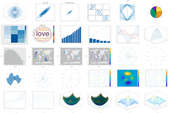
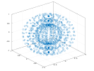
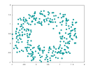
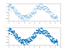
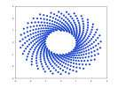
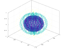
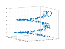
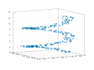
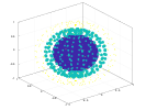
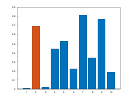
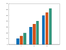
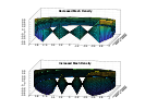
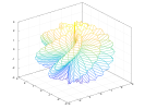
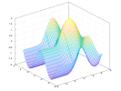
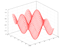
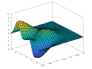
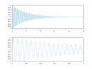
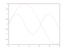
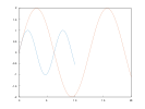
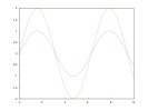
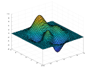
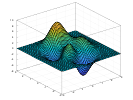
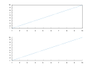
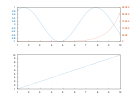
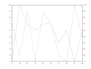
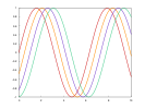
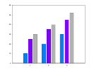
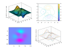
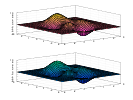
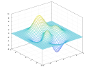
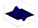
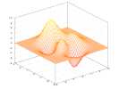
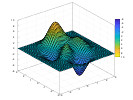
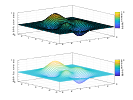
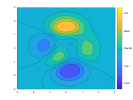
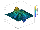
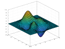
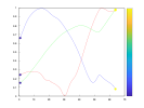
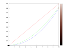
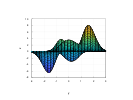
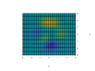
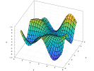
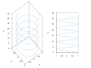
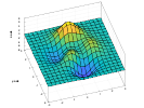
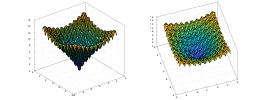
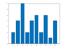
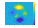
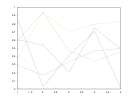
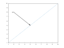
Data visualization can help programmers and scientists identify trends in their data and efficiently communicate these results with their peers. Modern C++ is being used for a variety of scientific applications, and this environment can benefit considerably from graphics libraries that attend the typical design goals toward scientific data visualization. Besides the option of exporting results to other environments, the customary alternatives in C++ are either non-dedicated libraries that depend on existing user interfaces or bindings to other languages. Matplot++ is a graphics library for data visualization that provides interactive plotting, means for exporting plots in high-quality formats for scientific publications, a compact syntax consistent with similar libraries, dozens of plot categories with specialized algorithms, multiple coding styles, and supports generic backends.













READ THE DOCUMENTATION FOR A QUICK START AND EXAMPLES































Vcpkg users can install Matplot++ with the matplotplusplus port:
vcpkg install matplotplusplus
This formula is a contribution to vcpkg by @myd7349.
Mac users can install Matplot++ with Homebrew:
brew install matplotplusplus
This formula is a contribution to Homebrew by Andrew Kane.
Matplot++ is available in the Arch User Repository
(AUR) as
matplotplusplus.
Note you can manually install the package by following the instructions on the
Arch Wiki
or use an AUR helper like
yay
(recommended for ease of install).
yay -S matplotplusplus
To discuss any issues related to this package refer to the comments section on
the AUR page of matplotplusplus here.
You can use Matplot++ directly in CMake projects as a subproject, without installing it. This is convenient if you are experimenting with this library for the first time or don't expect your users to have Matplot++ installed on their systems.
Check if you have Cmake 3.14+ installed:
cmake --version
Clone the whole project
git clone https://github.com/alandefreitas/matplotplusplus/
and add the subdirectory to your CMake project:
add_subdirectory(matplotplusplus)
When creating your executable, link the library to the targets you want:
add_executable(my_target main.cpp)
target_link_libraries(my_target PUBLIC matplot)
Add this header to your source files:
#include <matplot/matplot.h>
However, in larger projects, it's always recommended to look for Matplot++ with find_package before including it as a subdirectory to avoid ODR errors.
If you have CMake 3.21 or greater, you can use the system build preset to
build the package system-wide:
cmake --preset=system
cmake --build --preset=system
sudo cmake --install build/system
Alternatively, if the CMAKE_PREFIX_PATH environment variable is set to
$HOME/.local, then you can install it locally. This can be set in /etc/profile
or your shell config. This will not affect discovery of packages installed
system-wide.
export CMAKE_PREFIX_PATH="$HOME/.local"
This has the advantage of not
requiring sudo, and matplotplusplus will be installed in $HOME/.local.
cmake --preset=local
cmake --build --preset=local
cmake --install build/local
You can now use it from CMake with find_package:
find_package(Matplot++ REQUIRED)

target_link_libraries(<your target> Matplot++::matplot)
If you're using a version of CMake too old to support presets, then building with the system preset is equivilant to:
cmake -B build/system         \
    -DMATPLOTPP_BUILD_EXAMPLES=OFF      \
    -DMATPLOTPP_BUILD_SHARED_LIBS=ON    \
    -DMATPLOTPP_BUILD_TESTS=OFF         \
    -DCMAKE_BUILD_TYPE=Release \
    -DCMAKE_INTERPROCEDURAL_OPTIMIZATION=ON

cmake --build build/system
While building with the local preset is equivilant to:
cmake -B build/local                      \
    -DMATPLOTPP_BUILD_EXAMPLES=OFF                  \
    -DMATPLOTPP_BUILD_SHARED_LIBS=ON                \
    -DMATPLOTPP_BUILD_TESTS=OFF                     \
    -DCMAKE_BUILD_TYPE=Release            \
    -DCMAKE_INSTALL_PREFIX="$HOME/.local" \
    -DCMAKE_INTERPROCEDURAL_OPTIMIZATION=ON

cmake --build build/local
FetchContent is a CMake command that can automatically download the Matplot++ repository. Check if you have Cmake 3.14+ installed:
cmake --version
Include FetchContent in your CMake build script:
include(FetchContent)
Declare the source for the contents:
FetchContent_Declare(matplotplusplus
        GIT_REPOSITORY https://github.com/alandefreitas/matplotplusplus
        GIT_TAG origin/master) # or whatever tag you want
Let CMake download the repository and include it as a subdirectory.
FetchContent_GetProperties(matplotplusplus)
if(NOT matplotplusplus_POPULATED)
    FetchContent_Populate(matplotplusplus)
    add_subdirectory(${matplotplusplus_SOURCE_DIR} ${matplotplusplus_BINARY_DIR} EXCLUDE_FROM_ALL)
endif()
When creating your executable, link the library to the targets you want:
add_executable(my_target main.cpp)
target_link_libraries(my_target PUBLIC matplot)
Then add this header to your source files:
#include <matplot/matplot.h>
However, in larger projects, it's always recommended to look for Matplot++ with find_package before including it as a subdirectory to avoid ODR errors.
CPM.cmake is a nice wrapper around the CMake FetchContent function.
Check if you have Cmake 3.14+ installed:
cmake --version
Install CPM.cmake and then use this command to add Matplot++ to your build script:
CPMAddPackage(
    NAME matplotplusplus
    GITHUB_REPOSITORY alandefreitas/matplotplusplus
    GIT_TAG origin/master # or whatever tag you want
)
# ...
target_link_libraries(my_target PUBLIC matplot)
Then add this header to your source files:
#include <matplot/matplot.h>
However, in larger projects, it's always recommended to look for Matplot++ with find_package before including it as a subdirectory to avoid ODR errors.
You can use:
option(CPM_USE_LOCAL_PACKAGES "Try `find_package` before downloading dependencies" ON)
in your build script to let CPM.cmake do that for you.
If you have the library installed on your system, you can call find_package() from your CMake build script.
find_package(Matplot++ REQUIRED)
When creating your executable, link the library to the targets you want:
add_executable(my_target main.cpp)
target_link_libraries(my_target PUBLIC Matplot++::matplot)
Then add this header to your source files:
#include <matplot/matplot.h>
You can see a complete example in test/integration/CMakeLists.txt.
CMake should be able to locate the Matplot++Config.cmake script automatically if you installed the library under /usr/local/ (Linux / Mac OS). Unfortunately, there is no easy default directory for find_package on Windows.
!!! warning "Default directories"
By default, the library is likely to be in `/usr/local/` (Linux / Mac OS) or `C:/Program Files/` (Windows). The installer will try to find the directory where you usually keep your libraries but that's not always perfect.
!!! warning "Finding packages on Windows"
Unfortunately, CMake does not have a single default directory for packages on Windows like `/usr/local/lib`. If CMake cannot find Matplot++ on Windows or if you installed the library outside the default directory on Linux/Mac OS, there are a few [options](https://stackoverflow.com/questions/21314893/what-is-the-default-search-path-for-find-package-in-windows-using-cmake):

* **Environment Variables**: The most reliable way to set this default directory is through environment variables. You can create an environment variable `MATPLOTPP_DIR` and then add `$ENV{MATPLOTPP_DIR}` to the `HINTS` section of the `find_package` command. This tends to be more convenient than requiring the path on the command line every time. Starting with version 3.12, CMake now implicitly considers the `<PackageName>_Root` environment variable a HINT for every `find_package` call.
* **Package Registry**: CMake offers the [Package Registry](https://cmake.org/cmake/help/v3.5/manual/cmake-packages.7.html#package-registry) as an alternative mechanism for finding package locations. CMake maintains a list of package information in the Windows registry under `HKEY_CURRENT_USER\Software\Kitware\CMake\Packages\`.
* **Append CMAKE_MODULE_PATH**: You can append more directories to [`CMAKE_MODULE_PATH`](https://cmake.org/cmake/help/latest/variable/CMAKE_MODULE_PATH.html) with something like `list(APPEND CMAKE_MODULE_PATH "C:\\Program Files\\matplotplusplus 1.0.1")`. `CMAKE_MODULE_PATH` is a list of search paths for CMake modules to be loaded by the `include()` or `find_package()` commands.
* **Set the DIR variable directly**: Directly set the `Matplot++_DIR` variable with something like `set(Matplot++_DIR "C:\\Program Files\\matplotplusplus 1.0.1\\lib\\cmake\\Matplot++")`. This might be good enough for small local projects but it is hard-coding the directory in your build script. When your library gets out of your local environment, you need to choose one of the other options above (better) or make this variable an option and require the user to provide the directory on the command line every time (worse).
It's often useful to let your build script download Matplot++ when find_package fails. If using CPM.cmake, you can set the CPM_USE_LOCAL_PACKAGES option to try to find_package(Matplot++) before download Matplot++.
If using FetchContent, you can use the following pattern:
find_package(Matplot++ QUIET)
if(NOT Matplot++_FOUND)
    # Put your FetchContent or CPM.cmake script here
endif()
Get the binary package from the release section. These binaries refer to the last release version of Matplot++.
If you need a more recent version of Matplot++, you can download the binary packages from the CI artifacts or build the library from the source files.
C++17
Make sure your C++ compiler supports C++17:
=== "Ubuntu + GCC"
g++ --version
=== "Mac Os + Clang"
clang --version
=== "Windows + MSVC"
!!! warning ""
    * Visit the [Visual Studio](https://visualstudio.microsoft.com) website
    * Download Git from [https://git-scm.com/download/win](https://git-scm.com/download/win) and install it
The output should be something like:
=== "Ubuntu + GCC"
g++-8 (Ubuntu 8.4.0-1ubuntu1~18.04) 8.4.0
=== "Mac Os + Clang"
Apple clang version 11.0.0 (clang-1100.0.33.8)
=== "Windows + MSVC"
!!! warning ""
    * Visit the [Visual Studio](https://visualstudio.microsoft.com) website
    * Download Git from [https://git-scm.com/download/win](https://git-scm.com/download/win) and install it
If you need to update your compiler:
=== "Ubuntu + GCC"
# install GCC-8
sudo apt update
sudo apt install gcc-8
sudo apt install g++-8
To update to any other version, like GCC-9 or GCC-10:
sudo apt install build-essential
sudo add-apt-repository ppa:ubuntu-toolchain-r/test
sudo apt-get update
sudo apt install g++-10
Once you installed a newer version of GCC, you can link it to update-alternatives. For instance, if you have GCC-7 and GCC-10, you can link them with:
sudo update-alternatives --install /usr/bin/gcc gcc /usr/bin/gcc-7 7
sudo update-alternatives --install /usr/bin/g++ g++ /usr/bin/g++-7 7
sudo update-alternatives --install /usr/bin/gcc gcc /usr/bin/gcc-10 10
sudo update-alternatives --install /usr/bin/g++ g++ /usr/bin/g++-10 10
You can now use update-alternatives to set your default gcc and g++ to a more recent version:
update-alternatives --config g++
update-alternatives --config gcc
=== "Mac Os + Clang"
# download clang
curl --output clang.tar.xz -L https://github.com/llvm/llvm-project/releases/download/llvmorg-11.0.0/clang+llvm-11.0.0-x86_64-apple-darwin.tar.xz
mkdir clang
tar -xvJf clang.tar.xz -C clang

# copy files to /usr/local
cd clang/clang+llvm-11.0.0-x86_64-apple-darwin
sudo cp -R * /usr/local/

# update default compiler
export CXX=/usr/local/bin/clang++
=== "Windows + MSVC"
!!! warning ""
    * Visit the [Visual Studio](https://visualstudio.microsoft.com) website
    * Download Git from [https://git-scm.com/download/win](https://git-scm.com/download/win) and install it
CMake 3.14+
Also check your CMake version is at least 3.14+:
=== "Ubuntu + GCC"
cmake --version
=== "Mac Os + Clang"
cmake --version
=== "Windows + MSVC"
cmake --version
If CMake is not installed or its version is older than CMake 3.14, update it with
=== "Ubuntu + GCC"
sudo apt upgrade cmake
!!! warning ""
    Alternatively, download the most recent version from [cmake.org](https://cmake.org/).
=== "Mac Os + Clang"
brew upgrade cmake
!!! warning "Homebrew"
    If this command fails because you don't have [Homebrew](https://brew.sh) on your computer, you can install it with
/bin/bash -c "$(curl -fsSL https://raw.githubusercontent.com/Homebrew/install/master/install.sh)"
    or you can follow the instructions in [https://brew.sh](https://brew.sh).


!!! warning ""
    Alternatively, download the most recent version from [cmake.org](https://cmake.org/).
=== "Windows + MSVC"
!!! warning ""
    Download the most recent version from [cmake.org](https://cmake.org/).
Gnuplot 5.2.6+
Install Gnuplot 5.2.6+ (Required at runtime)
=== "Ubuntu + GCC"
sudo apt update
sudo apt install gnuplot
!!! note ""
    Or download the latest version from [www.gnuplot.info](http://www.gnuplot.info). If you're using an installer, make sure you mark the option "Add application directory to your PATH environment variable".
=== "Mac Os + Clang"
brew install gnuplot
!!! note ""
    Or download the latest version from [www.gnuplot.info](http://www.gnuplot.info). If you're using an installer, make sure you mark the option "Add application directory to your PATH environment variable".
=== "Windows + MSVC"
!!! warning ""
    Download Gnuplot from [www.gnuplot.info](http://www.gnuplot.info) and install it.

    If you're using the Gnuplot installer, make sure you mark the option "Add application directory to your PATH environment variable"

!!! warning "Windows Gnuplot Terminals"

    If the Matplot++ examples don't display without console errors and gnuplot running, try to re-install Gnuplot with the wxt terminal.
Optional Dependencies
The build script will also look for these optional dependencies for manipulating images:
Embedded Dependencies
There are two dependencies in source/3rd_party. These dependencies are bundled, so you don't have to worry about them:
You can define MATPLOTPP_WITH_SYSTEM_NODESOUP=ON or MATPLOTPP_WITH_SYSTEM_CIMG=ON in the cmake command line to use a system-provided version of these dependencies.
OpenGL Dependencies
There's an extra target matplot_opengl with the experimental OpenGL backend. You need to define MATPLOTPP_BUILD_EXPERIMENTAL_OPENGL_BACKEND=ON in the CMake command line to build that target. In that case, the build script will also look for these extra dependencies:
If these dependencies are not found, the build script will download them. In any case, you can install these dependencies with:
=== "Ubuntu + GCC"
sudo apt-get install libglfw3-dev
=== "Mac Os + Clang"
!!! note ""
    Download GLFW3 from https://www.glfw.org
=== "Windows + MSVC"
!!! note ""
    Download GLFW3 from https://www.glfw.org
You can also see all dependencies in source/3rd_party/CMakeLists.txt.
Building Examples
This will build the examples in the build/examples directory:
=== "Ubuntu + GCC"
mkdir build
cd build
cmake .. -DCMAKE_BUILD_TYPE=Release -DCMAKE_CXX_FLAGS="-O2"
sudo cmake --build . --parallel 2 --config Release
=== "Mac Os + Clang"
mkdir build
cd build
cmake .. -DCMAKE_BUILD_TYPE=Release -DCMAKE_CXX_FLAGS="-O2"
cmake --build . --parallel 2 --config Release
=== "Windows + MSVC"
mkdir build
cd build
cmake .. -DCMAKE_BUILD_TYPE=Release -DCMAKE_CXX_FLAGS="/O2"
cmake --build . --parallel 2 --config Release
!!! hint "Parallel Build"
Replace --parallel 2 with --parallel <number of cores in your machine>
!!! note "Setting C++ Compiler"
If your C++ compiler that supports C++17 is not your default compiler, make sure you provide CMake with the compiler location with the DCMAKE_C_COMPILER and DCMAKE_CXX_COMPILER options. For instance:
cmake .. -DCMAKE_BUILD_TYPE=Release -DCMAKE_CXX_FLAGS="-O2" -DCMAKE_C_COMPILER=/usr/bin/gcc-8 -DCMAKE_CXX_COMPILER=/usr/bin/g++-8
Installing
You can 1) use -DMATPLOTPP_BUILD_EXAMPLES=OFF -DMATPLOTPP_BUILD_TESTS=OFF to bypass the examples and tests, and then 2) cmake --install . to install Matplot++ on your system:
=== "Ubuntu + GCC"
mkdir build
cd build
cmake .. -DCMAKE_BUILD_TYPE=Release -DCMAKE_CXX_FLAGS="-O2" -DMATPLOTPP_BUILD_EXAMPLES=OFF -DMATPLOTPP_BUILD_TESTS=OFF
sudo cmake --build . --parallel 2 --config Release
sudo cmake --install .
=== "Mac Os + Clang"
mkdir build
cd build
cmake .. -DCMAKE_BUILD_TYPE=Release -DCMAKE_CXX_FLAGS="-O2" -DMATPLOTPP_BUILD_EXAMPLES=OFF -DMATPLOTPP_BUILD_TESTS=OFF
cmake --build . --parallel 2 --config Release
cmake --install .
=== "Windows + MSVC"
mkdir build
cd build
cmake .. -DCMAKE_BUILD_TYPE=Release -DCMAKE_CXX_FLAGS="/O2" -DMATPLOTPP_BUILD_EXAMPLES=OFF -DMATPLOTPP_BUILD_TESTS=OFF
cmake --build . --parallel 2 --config Release
cmake --install .
!!! hint "Parallel Build"
Replace --parallel 2 with --parallel <number of cores in your machine>
Create Packages
You can also create the binary packages to install Matplot++ on other systems:
=== "Ubuntu + GCC"
sudo cpack .
=== "Mac Os + Clang"
cpack .
=== "Windows + MSVC"
cpack .
Line Plot | Line Plot 3D | Stairs | Error Bars | Area | Loglog Plot | Semilogx Plot | Semilogy Plot | Function Plot | Function Plot 3D | Implicit function
!!! tip Use these examples to understand how to quickly use the library for data visualization. If you are interested in understanding how the library works, you can later read the details in the complete article.
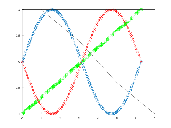
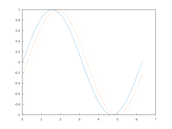
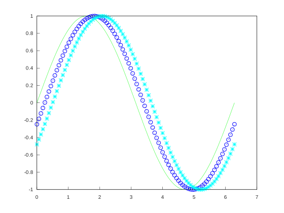
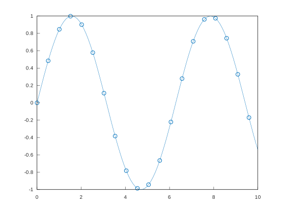
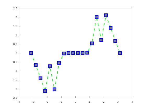
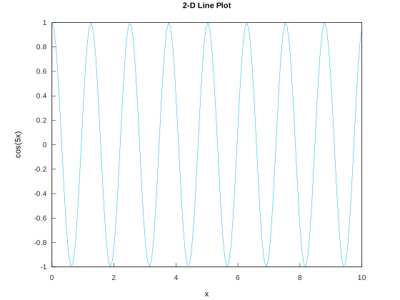
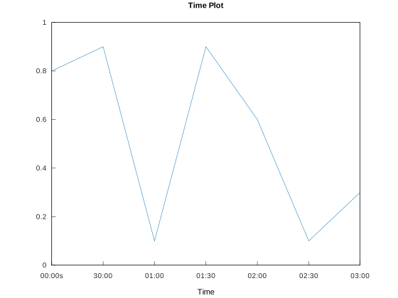
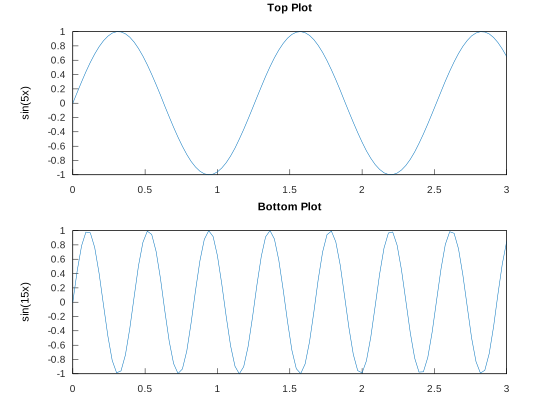
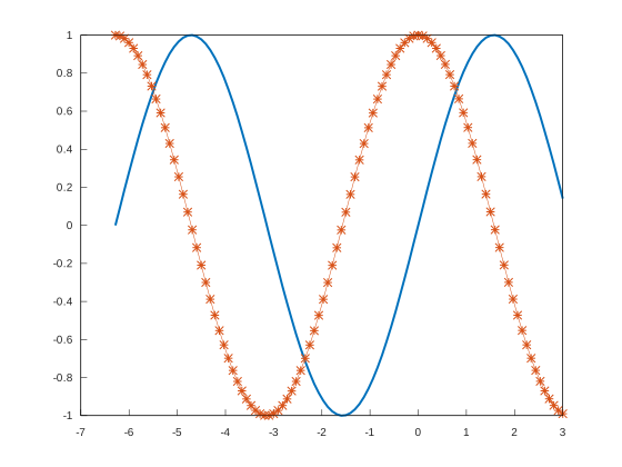
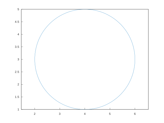
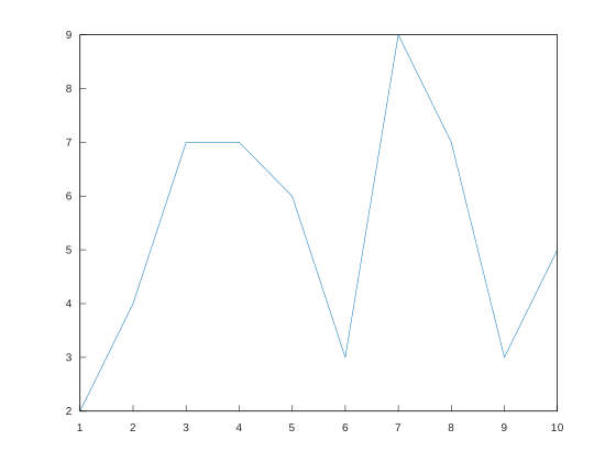
plot(x,y);
Where x and y are are any value ranges.
READ THE DOCUMENTATION TO SEE THESE EXAMPLES WITH THE IMAGES
=== "Plot"
=== "C++"
--8<-- "examples/line_plot/plot/plot_1.cpp"
!!! tip
Setters return a reference to *this to allow method chaining:
plot(x,y)->line_width(2).color("red");
!!! tip These examples use free-standing functions to create plots. You can also use a object-oriented style for plots. We discuss these coding styles in the Section Coding Styles.
More Examples:
===! "Plot"
=== "C++"
--8<-- "examples/line_plot/plot/plot_2.cpp"
===! "Plot"
=== "C++"
--8<-- "examples/line_plot/plot/plot_3.cpp"
===! "Plot"
=== "C++"
--8<-- "examples/line_plot/plot/plot_4.cpp"
===! "Plot"
=== "C++"
--8<-- "examples/line_plot/plot/plot_5.cpp"
===! "Plot"
=== "C++"
--8<-- "examples/line_plot/plot/plot_6.cpp"
===! "Plot"
=== "C++"
--8<-- "examples/line_plot/plot/plot_7.cpp"
===! "Plot"
=== "C++"
--8<-- "examples/line_plot/plot/plot_8.cpp"
===! "Plot"
=== "C++"
--8<-- "examples/line_plot/plot/plot_9.cpp"
===! "Plot"
=== "C++"
--8<-- "examples/line_plot/plot/plot_10.cpp"
===! "Plot"
=== "C++"
--8<-- "examples/line_plot/plot/plot_11.cpp"
===! "Plot"
=== "C++"
--8<-- "examples/line_plot/plot/plot_12.cpp"
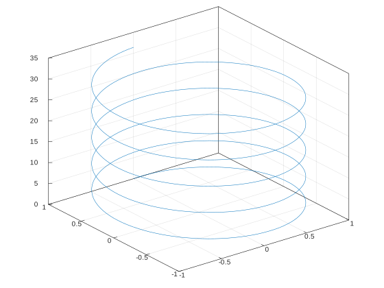
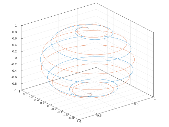
plot3(x,y);
=== "Plot"
=== "C++"
--8<-- "examples/line_plot/plot3/plot3_1.cpp"
!!! tip With method chaining:
plot3(x,y)->line_width(2).color("red");
More Examples:
===! "Plot"
=== "C++"
--8<-- "examples/line_plot/plot3/plot3_2.cpp"
===! "Plot"
=== "C++"
--8<-- "examples/line_plot/plot3/plot3_3.cpp"
===! "Plot"
=== "C++"
--8<-- "examples/line_plot/plot3/plot3_4.cpp"
===! "Plot"
=== "C++"
--8<-- "examples/line_plot/plot3/plot3_5.cpp"
===! "Plot"
=== "C++"
--8<-- "examples/line_plot/plot3/plot3_7.cpp"
===! "Plot"
=== "C++"
--8<-- "examples/line_plot/plot3/plot3_8.cpp"
===! "Plot"
=== "C++"
--8<-- "examples/line_plot/plot3/plot3_9.cpp"
===! "Plot"
=== "C++"
--8<-- "examples/line_plot/plot3/plot3_10.cpp"
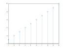
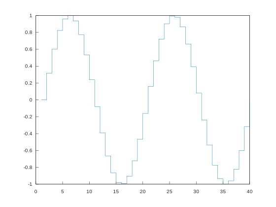
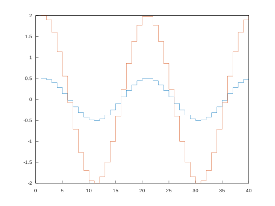
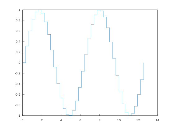
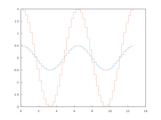
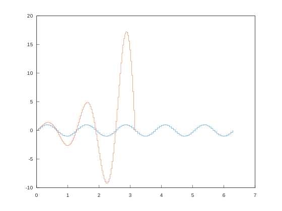
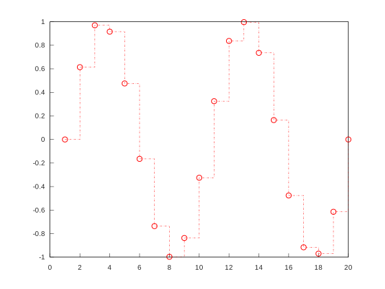
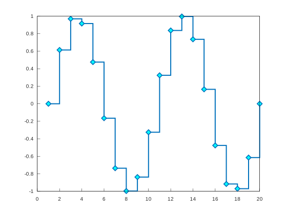
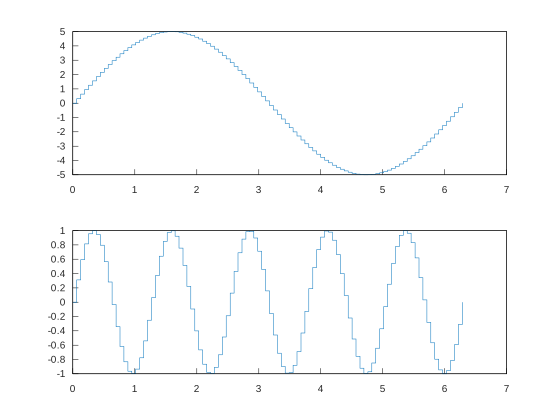
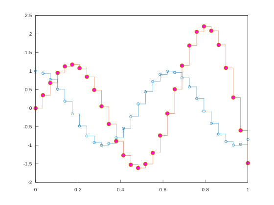
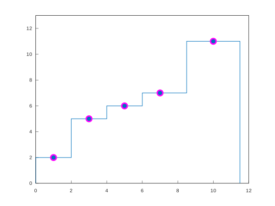
stairs(x,y);
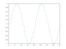
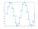
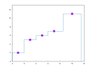
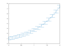
The stair object renders the line with stairs between data points to denote discrete data.
More Examples:
===! "Plot"
=== "C++"
--8<-- "examples/line_plot/stairs/stairs_2.cpp"
More Examples:
===! "Plot"
=== "C++"
--8<-- "examples/line_plot/stairs/stairs_3.cpp"
===! "Plot"
=== "C++"
--8<-- "examples/line_plot/stairs/stairs_4.cpp"
===! "Plot"
=== "C++"
--8<-- "examples/line_plot/stairs/stairs_5.cpp"
===! "Plot"
=== "C++"
--8<-- "examples/line_plot/stairs/stairs_6.cpp"
===! "Plot"
=== "C++"
--8<-- "examples/line_plot/stairs/stairs_7.cpp"
===! "Plot"
=== "C++"
--8<-- "examples/line_plot/stairs/stairs_8.cpp"
===! "Plot"
=== "C++"
--8<-- "examples/line_plot/stairs/stairs_9.cpp"
===! "Plot"
=== "C++"
--8<-- "examples/line_plot/stairs/stairs_10.cpp"
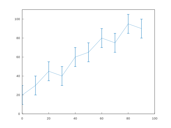
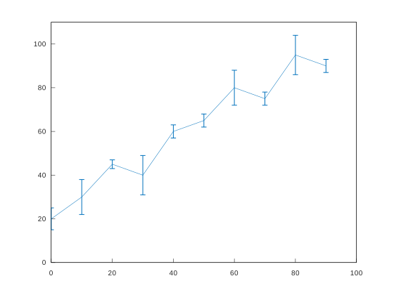
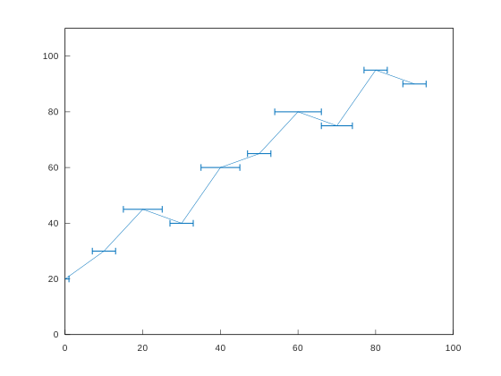
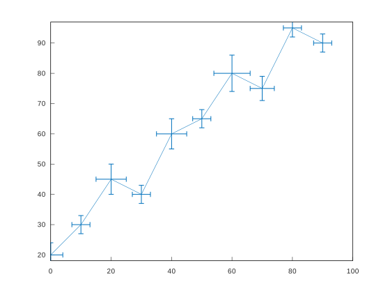
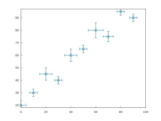
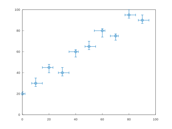
errorbar(x,y,err);
More Examples:
===! "Plot"
=== "C++"
--8<-- "examples/line_plot/errorbar/errorbar_1.cpp"
More Examples:
===! "Plot"
=== "C++"
--8<-- "examples/line_plot/errorbar/errorbar_2.cpp"
===! "Plot"
=== "C++"
--8<-- "examples/line_plot/errorbar/errorbar_3.cpp"
===! "Plot"
=== "C++"
--8<-- "examples/line_plot/errorbar/errorbar_4.cpp"
===! "Plot"
=== "C++"
--8<-- "examples/line_plot/errorbar/errorbar_5.cpp"
===! "Plot"
=== "C++"
--8<-- "examples/line_plot/errorbar/errorbar_6.cpp"
===! "Plot"
=== "C++"
--8<-- "examples/line_plot/errorbar/errorbar_7.cpp"
===! "Plot"
=== "C++"
--8<-- "examples/line_plot/errorbar/errorbar_8.cpp"
===! "Plot"
=== "C++"
--8<-- "examples/line_plot/errorbar/errorbar_9.cpp"
===! "Plot"
=== "C++"
--8<-- "examples/line_plot/errorbar/errorbar_10.cpp"
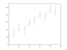
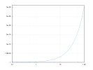
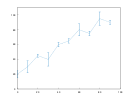
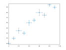
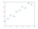
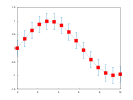
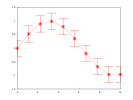
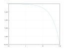
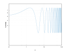
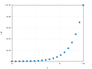
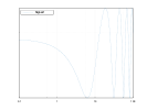
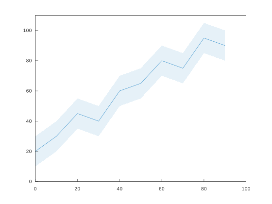
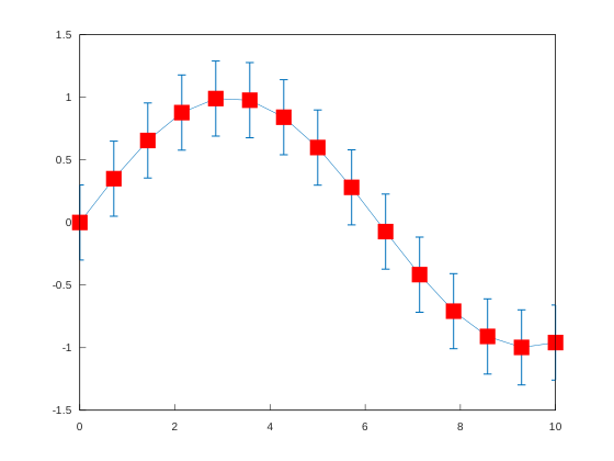
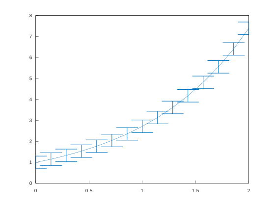
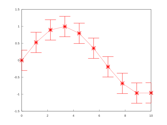
The error bar object includes extra lines to represent error around data points. Log plots are utility functions that adjust the x or y axes to a logarithmic scale.
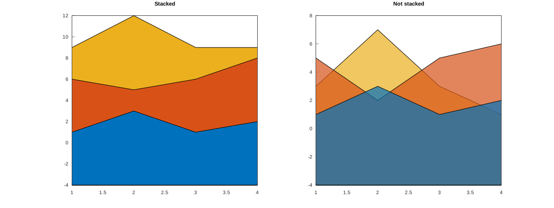
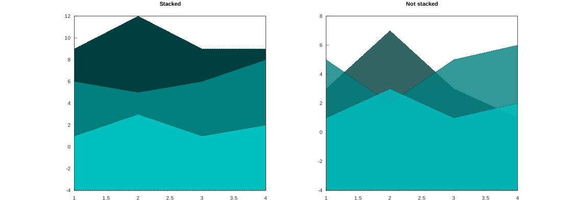
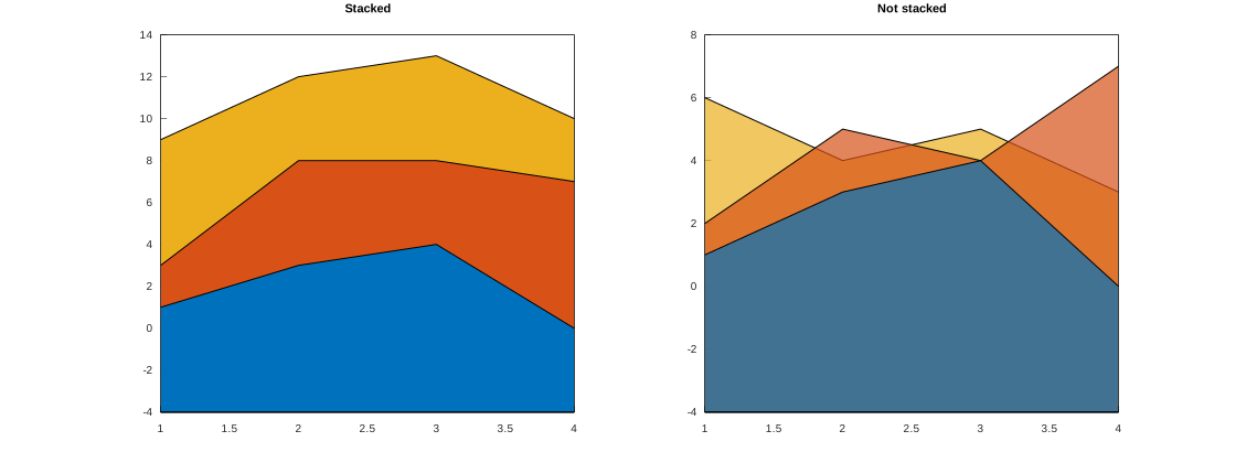
area(Y);
More Examples:
===! "Plot"
=== "C++"
--8<-- "examples/line_plot/area/area_1.cpp"
More Examples:
===! "Plot"
=== "C++"
--8<-- "examples/line_plot/area/area_2.cpp"
===! "Plot"
=== "C++"
--8<-- "examples/line_plot/area/area_3.cpp"
===! "Plot"
=== "C++"
--8<-- "examples/line_plot/area/area_4.cpp"
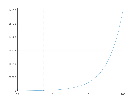
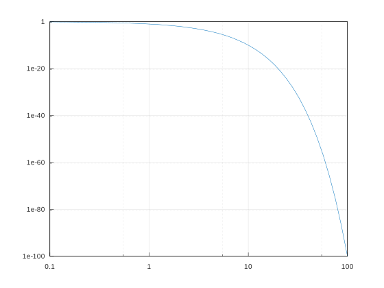
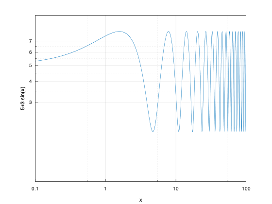
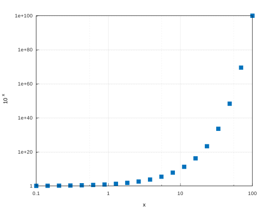
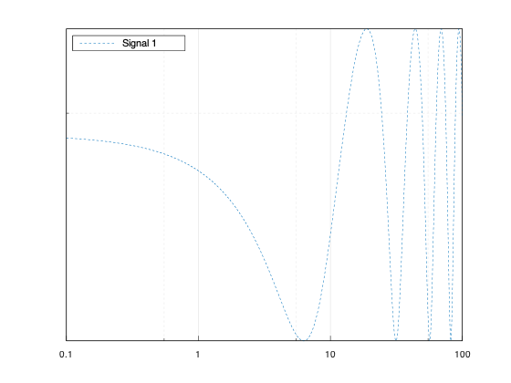
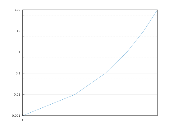
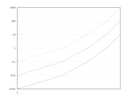
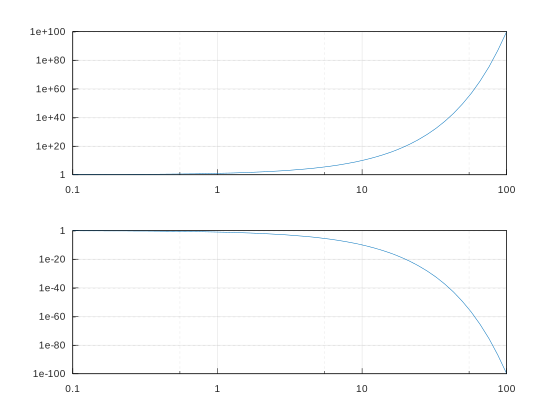
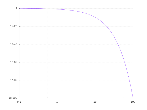
loglog(x,y);
More Examples:
===! "Plot"
=== "C++"
--8<-- "examples/line_plot/loglog/loglog_1.cpp"
More Examples:
===! "Plot"
=== "C++"
--8<-- "examples/line_plot/loglog/loglog_2.cpp"
===! "Plot"
=== "C++"
--8<-- "examples/line_plot/loglog/loglog_3.cpp"
===! "Plot"
=== "C++"
--8<-- "examples/line_plot/loglog/loglog_4.cpp"
===! "Plot"
=== "C++"
--8<-- "examples/line_plot/loglog/loglog_5.cpp"
===! "Plot"
=== "C++"
--8<-- "examples/line_plot/loglog/loglog_6.cpp"
===! "Plot"
=== "C++"
--8<-- "examples/line_plot/loglog/loglog_7.cpp"
===! "Plot"
=== "C++"
--8<-- "examples/line_plot/loglog/loglog_8.cpp"
===! "Plot"
=== "C++"
--8<-- "examples/line_plot/loglog/loglog_9.cpp"
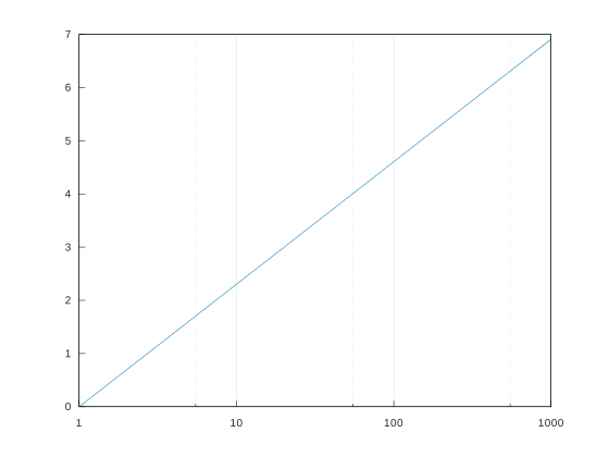
semilogx(x,y);
===! "Plot"
=== "C++"
```cpp
--8<-- "examples/line_plot/semilogx/semilogx_1.cpp"
```
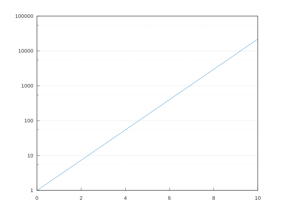
semilogy(x,y);
===! "Plot"
=== "C++"
--8<-- "examples/line_plot/semilogy/semilogy_1.cpp"
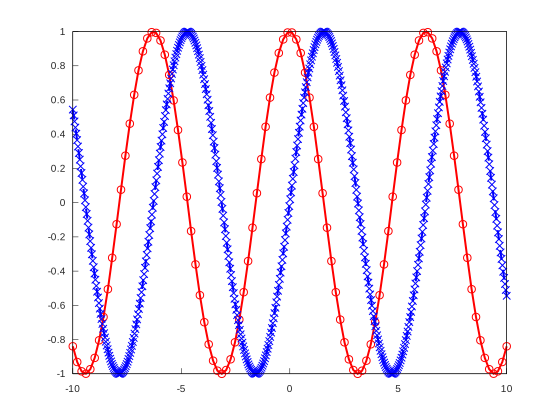
fplot(fx);
More Examples:
===! "Plot"
=== "C++"
--8<-- "examples/line_plot/fplot/fplot_1.cpp"
More Examples:
===! "Plot"
=== "C++"
--8<-- "examples/line_plot/fplot/fplot_2.cpp"
===! "Plot"
=== "C++"
--8<-- "examples/line_plot/fplot/fplot_3.cpp"
===! "Plot"
=== "C++"
--8<-- "examples/line_plot/fplot/fplot_4.cpp"
===! "Plot"
=== "C++"
```cpp
--8<-- "examples/line_plot/fplot/fplot_5.cpp"
```
===! "Plot"
=== "C++"
```cpp
--8<-- "examples/line_plot/fplot/fplot_6.cpp"
```
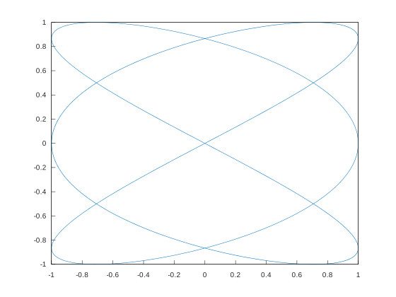
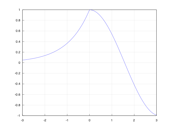
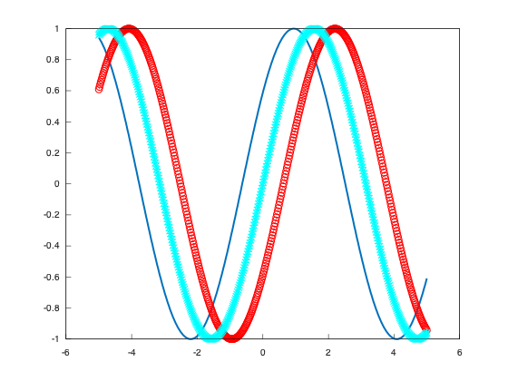
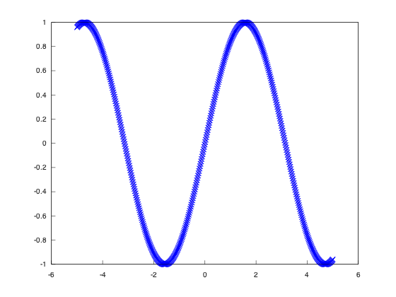
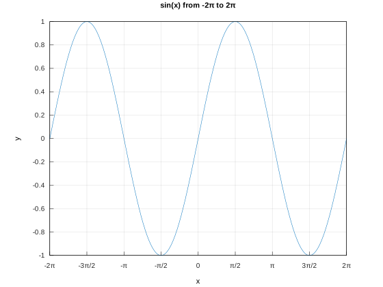
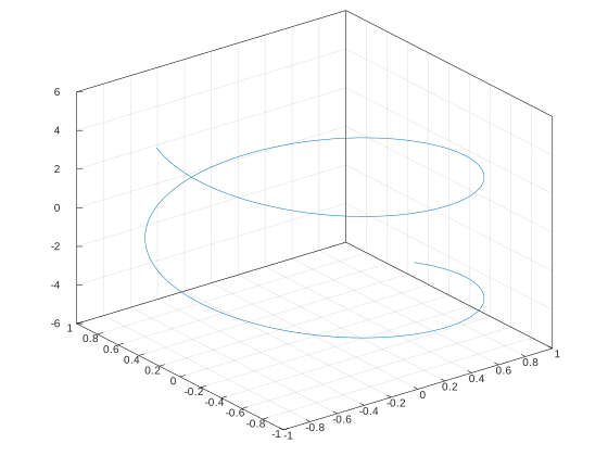
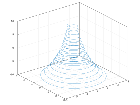
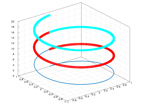
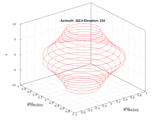
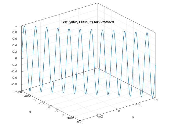
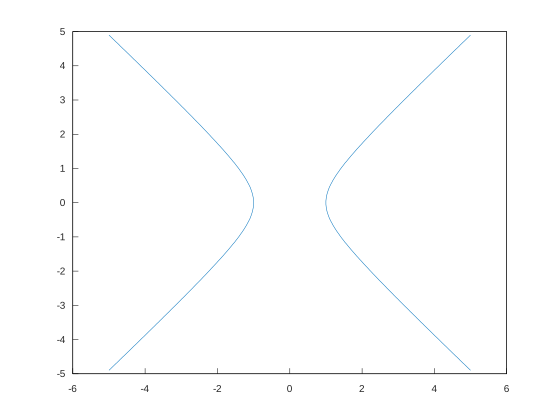
Instead of storing data points, the objects function line and string function store a function as a lambda function or as a string with an expression. These objects use lazy evaluation to generate absolute data points. The data is generated only when the draw function is called.
fplot(fxy);
More Examples:
===! "Plot"
=== "C++"
```cpp
--8<-- "examples/line_plot/fplot3/fplot3_1.cpp"
`````
More Examples:
===! "Plot"
=== "C++"
```cpp
--8<-- "examples/line_plot/fplot3/fplot3_2.cpp"
```
===! "Plot"
=== "C++"
```cpp
--8<-- "examples/line_plot/fplot3/fplot3_3.cpp"
```
===! "Plot"
=== "C++"
```cpp
--8<-- "examples/line_plot/fplot3/fplot3_4.cpp"
```
===! "Plot"
=== "C++"
```cpp
--8<-- "examples/line_plot/fplot3/fplot3_5.cpp"
```
fplot(fxy);
More Examples:
===! "Plot"
=== "C++"
```cpp
--8<-- "examples/line_plot/fimplicit/fimplicit_1.cpp"
```
More Examples:
===! "Plot"
=== "C++"
```cpp
--8<-- "examples/line_plot/fimplicit/fimplicit_2.cpp"
```
===! "Plot"
=== "C++"
```cpp
--8<-- "examples/line_plot/fimplicit/fimplicit_3.cpp"
```
===! "Plot"
=== "C++"
```cpp
--8<-- "examples/line_plot/fimplicit/fimplicit_4.cpp"
```
Histogram | Boxplot | Scatter Plot | Scatter Plot 3D | Binned Scatter Plots | Plot Matrix | Parallel Coordinates | Pie Chart | Heatmap | Word Cloud
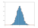
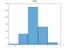
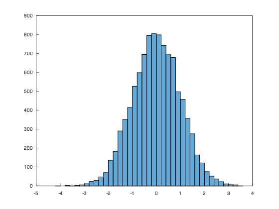
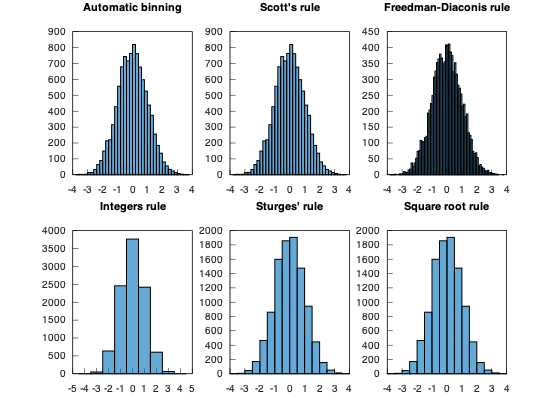
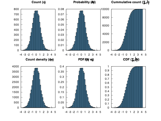
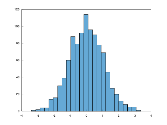
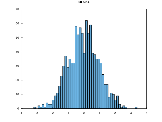
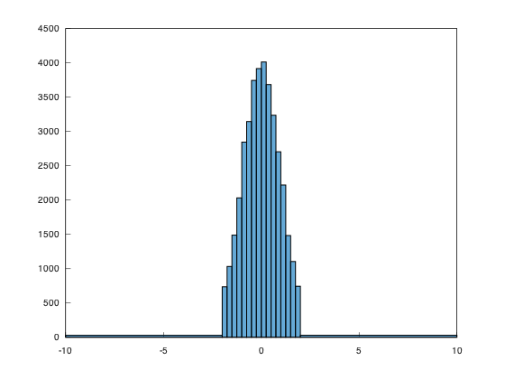
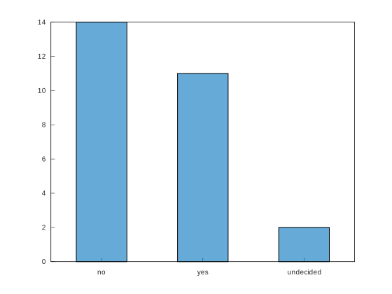
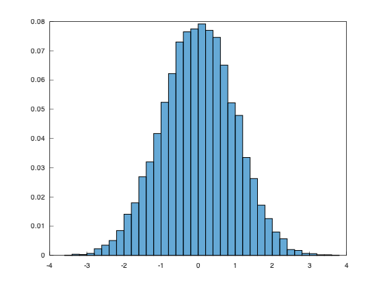
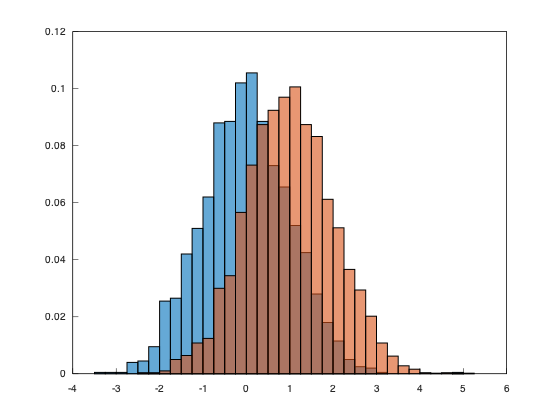
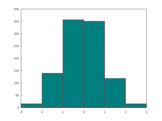
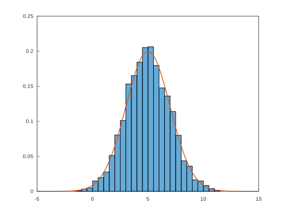
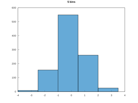
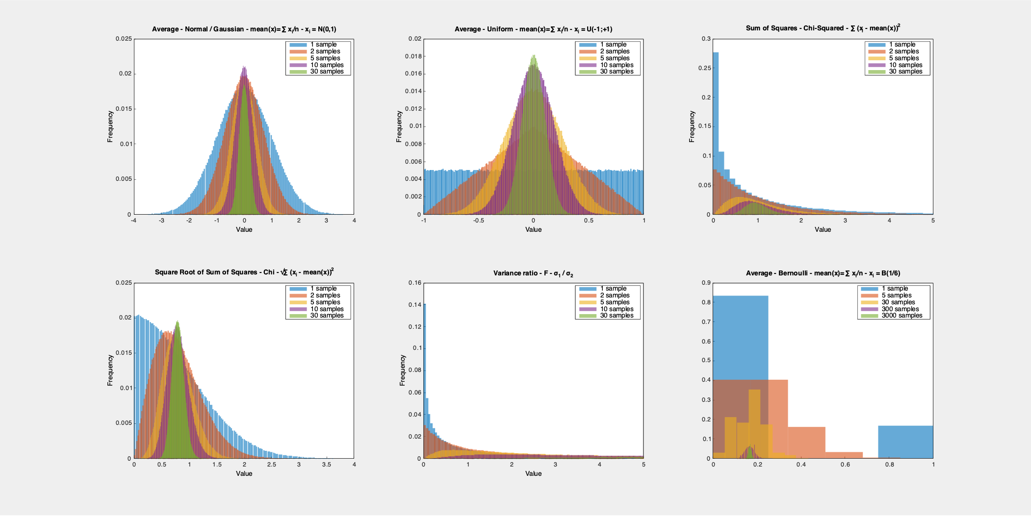
The histogram object creates the histogram edges and bins when the draw function is called for the first time with lazy evaluation. Lazy evaluation avoids calculating edges unnecessarily in case the user changes the object parameters before calling draw. This object includes several algorithms for automatically delimiting the edges and bins for the histograms.
hist(data);
More Examples:
===! "Plot"
=== "C++"
```cpp
--8<-- "examples/data_distribution/histogram/histogram_1.cpp"
```
More Examples:
===! "Plot"
=== "C++"
```cpp
--8<-- "examples/data_distribution/histogram/histogram_2.cpp"
```
===! "Plot"
=== "C++"
```cpp
--8<-- "examples/data_distribution/histogram/histogram_3.cpp"
```
===! "Plot"
=== "C++"
```cpp
--8<-- "examples/data_distribution/histogram/histogram_4.cpp"
```
===! "Plot"
=== "C++"
```cpp
--8<-- "examples/data_distribution/histogram/histogram_5.cpp"
```
===! "Plot"
=== "C++"
```cpp
--8<-- "examples/data_distribution/histogram/histogram_6.cpp"
```
===! "Plot"
=== "C++"
```cpp
--8<-- "examples/data_distribution/histogram/histogram_7.cpp"
```
===! "Plot"
=== "C++"
```cpp
--8<-- "examples/data_distribution/histogram/histogram_8.cpp"
```
===! "Plot"
=== "C++"
```cpp
--8<-- "examples/data_distribution/histogram/histogram_9.cpp"
```
===! "Plot"
=== "C++"
```cpp
--8<-- "examples/data_distribution/histogram/histogram_10.cpp"
```
===! "Plot"
=== "C++"
```cpp
--8<-- "examples/data_distribution/histogram/histogram_11.cpp"
```
===! "Plot"
=== "C++"
```cpp
--8<-- "examples/data_distribution/histogram/histogram_12.cpp"
```
===! "Plot"
=== "C++"
```cpp
--8<-- "examples/data_distribution/histogram/histogram_14.cpp"
```
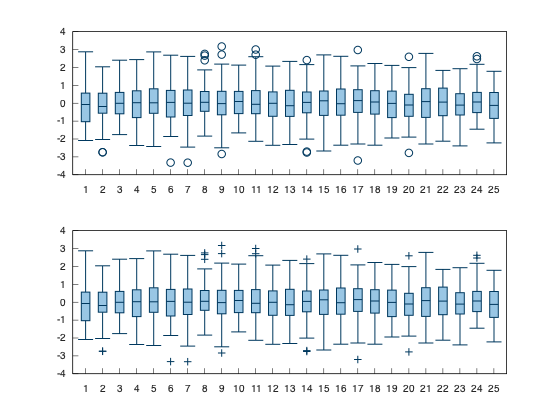
boxplot(data);
More Examples:
===! "Plot"
=== "C++"
```cpp
--8<-- "examples/data_distribution/boxplot/boxplot_1.cpp"
```
More Examples:
===! "Plot"
=== "C++"
```cpp
--8<-- "examples/data_distribution/boxplot/boxplot_2.cpp"
```
===! "Plot"
=== "C++"
```cpp
--8<-- "examples/data_distribution/boxplot/boxplot_3.cpp"
```
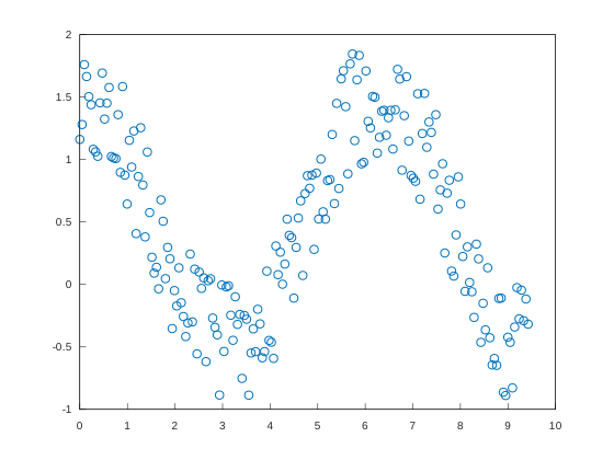
scatter(x,y);
More Examples:
===! "Plot"
=== "C++"
```cpp
--8<-- "examples/data_distribution/scatter/scatter_1.cpp"
```
More Examples:
===! "Plot"
=== "C++"
```cpp
--8<-- "examples/data_distribution/scatter/scatter_2.cpp"
```
===! "Plot"
=== "C++"
```cpp
--8<-- "examples/data_distribution/scatter/scatter_3.cpp"
```
===! "Plot"
=== "C++"
```cpp
--8<-- "examples/data_distribution/scatter/scatter_4.cpp"
```
===! "Plot"
=== "C++"
```cpp
--8<-- "examples/data_distribution/scatter/scatter_5.cpp"
```
===! "Plot"
=== "C++"
```cpp
--8<-- "examples/data_distribution/scatter/scatter_6.cpp"
```
===! "Plot"
=== "C++"
```cpp
--8<-- "examples/data_distribution/scatter/scatter_7.cpp"
```
===! "Plot"
=== "C++"
```cpp
--8<-- "examples/data_distribution/scatter/scatter_8.cpp"
```
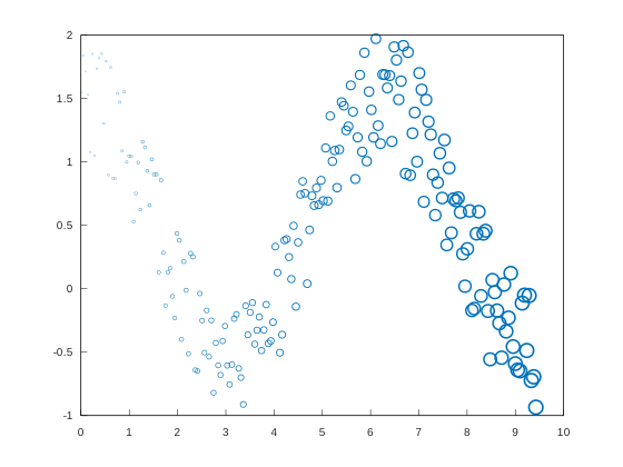
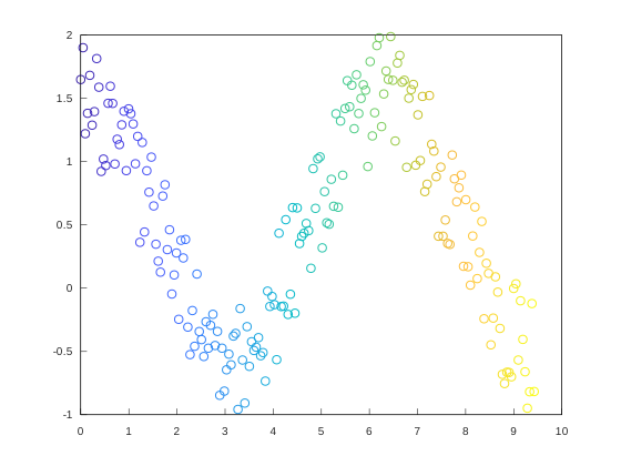
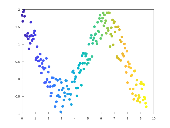
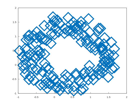
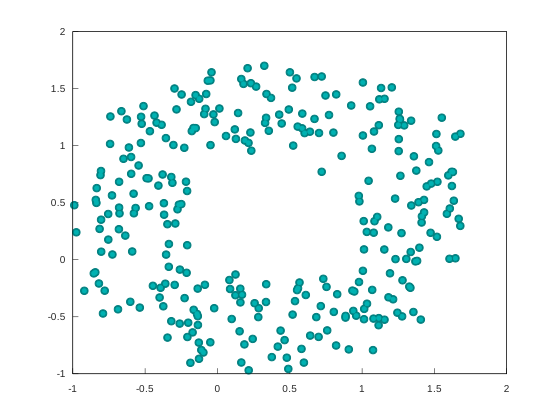
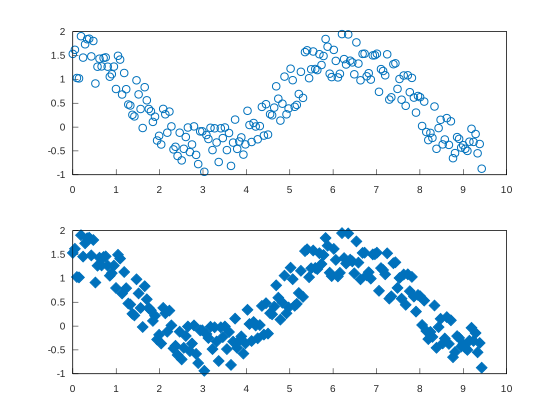
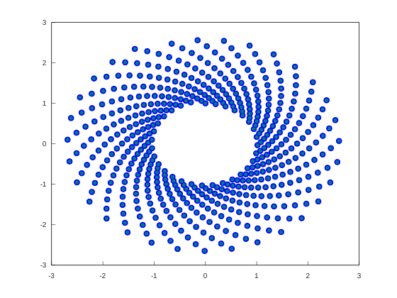
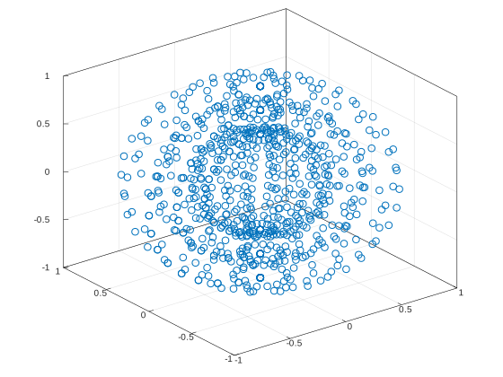
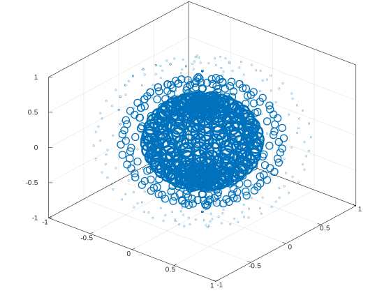
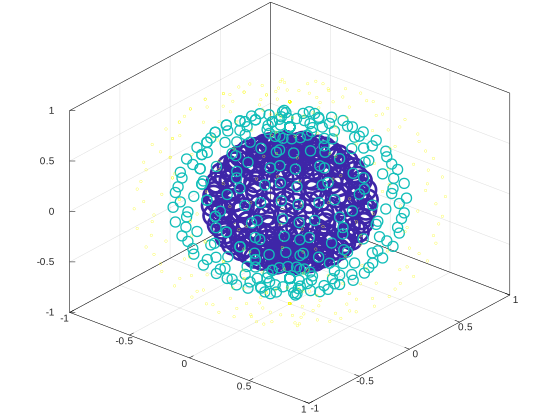
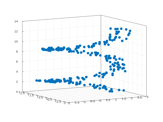
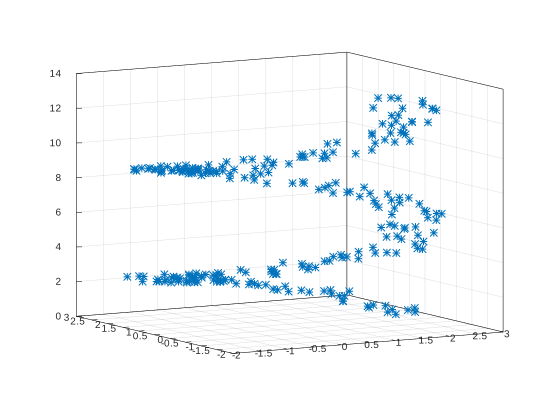
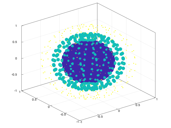
Scatter plots also depend on the line object. As the line object can represent lines with markers, the scatter function simply creates markers without the lines.
scatter(x,y,z);
More Examples:
===! "Plot"
=== "C++"
```cpp
--8<-- "examples/data_distribution/scatter3/scatter3_1.cpp"
```
More Examples:
===! "Plot"
=== "C++"
```cpp
--8<-- "examples/data_distribution/scatter3/scatter3_2.cpp"
```
===! "Plot"
=== "C++"
```cpp
--8<-- "examples/data_distribution/scatter3/scatter3_3.cpp"
```
===! "Plot"
=== "C++"
```cpp
--8<-- "examples/data_distribution/scatter3/scatter3_4.cpp"
```
===! "Plot"
=== "C++"
```cpp
--8<-- "examples/data_distribution/scatter3/scatter3_5.cpp"
```
===! "Plot"
=== "C++"
```cpp
--8<-- "examples/data_distribution/scatter3/scatter3_6.cpp"
```
binscatter(x,y);
More Examples:
===! "Plot"
=== "C++"
```cpp
--8<-- "examples/data_distribution/binscatter/binscatter_1.cpp"
```
More Examples:
===! "Plot"
=== "C++"
```cpp
--8<-- "examples/data_distribution/binscatter/binscatter_2.cpp"
```
===! "Plot"
=== "C++"
```cpp
--8<-- "examples/data_distribution/binscatter/binscatter_3.cpp"
```
===! "Plot"
=== "C++"
```cpp
--8<-- "examples/data_distribution/binscatter/binscatter_4.cpp"
```
===! "Plot"
=== "C++"
```cpp
--8<-- "examples/data_distribution/binscatter/binscatter_5.cpp"
```
===! "Plot"
=== "C++"
```cpp
--8<-- "examples/data_distribution/binscatter/binscatter_6.cpp"
```
===! "Plot"
=== "C++"
```cpp
--8<-- "examples/data_distribution/binscatter/binscatter_7.cpp"
```
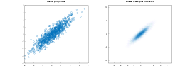
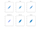
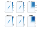
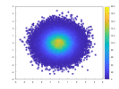
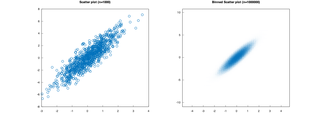
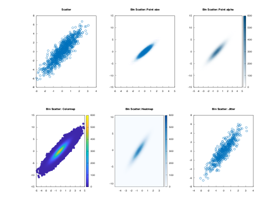
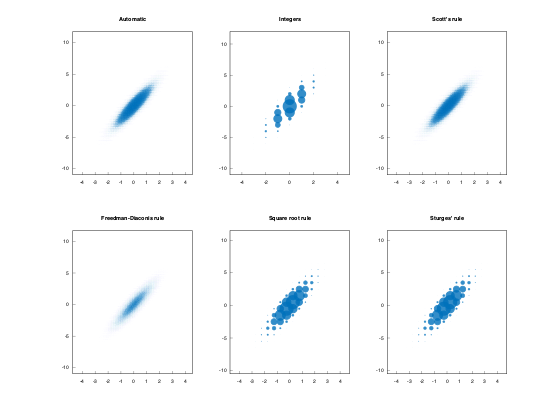
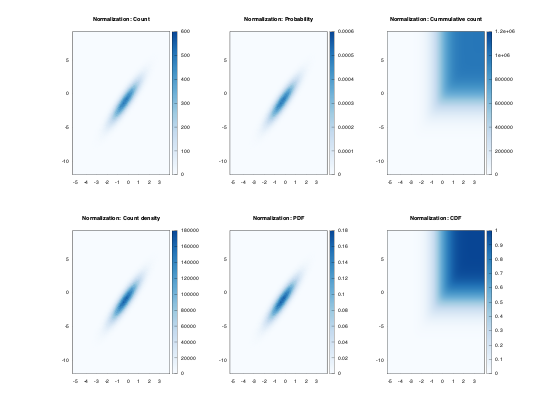
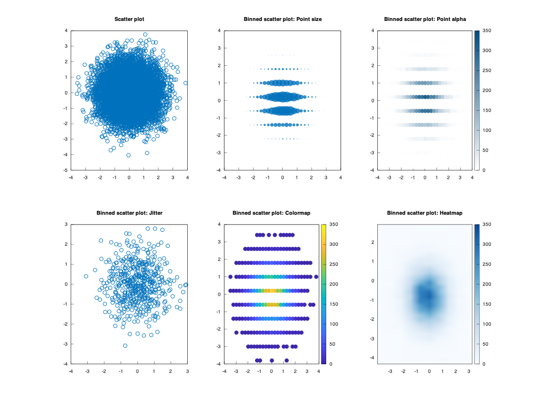
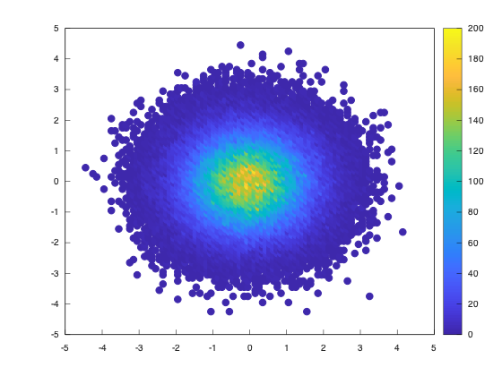
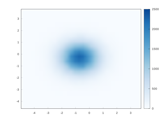
Binned scatter plots use variations of the histogram algorithms of the previous section as an extra step to place all the data into two-dimensional bins that can be represented with varying colors or sizes. This is useful when there are so many data points that a scatter plot would be impractical for visualizing the data.
plotmatrix(X);
More Examples:
===! "Plot"
=== "C++"
```cpp
--8<-- "examples/data_distribution/plotmatrix/plotmatrix_1.cpp"
```
More Examples:
===! "Plot"
=== "C++"
```cpp
--8<-- "examples/data_distribution/plotmatrix/plotmatrix_2.cpp"
```
===! "Plot"
=== "C++"
```cpp
--8<-- "examples/data_distribution/plotmatrix/plotmatrix_3.cpp"
```
===! "Plot"
=== "C++"
```cpp
--8<-- "examples/data_distribution/plotmatrix/plotmatrix_4.cpp"
```
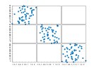
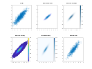
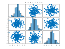
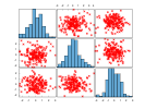
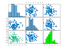
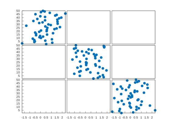
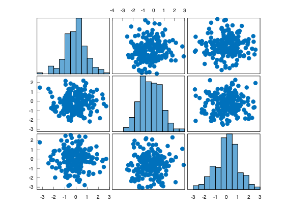
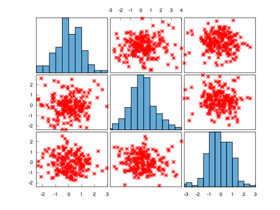
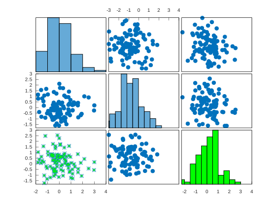
The Plot Matrix subcategory is a combination of histograms and scatter plots. It creates a matrix of axes objects on the figure and creates a scatter plot for each pair of data sets.
parallelplot(X);
More Examples:
===! "Plot"
=== "C++"
```cpp
--8<-- "examples/data_distribution/parallelplot/parallelplot_1.cpp"
```
More Examples:
===! "Plot"
=== "C++"
```cpp
--8<-- "examples/data_distribution/parallelplot/parallelplot_2.cpp"
```
===! "Plot"
=== "C++"
```cpp
--8<-- "examples/data_distribution/parallelplot/parallelplot_3.cpp"
```
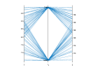
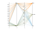
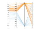
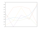
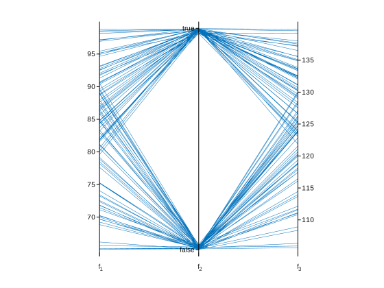
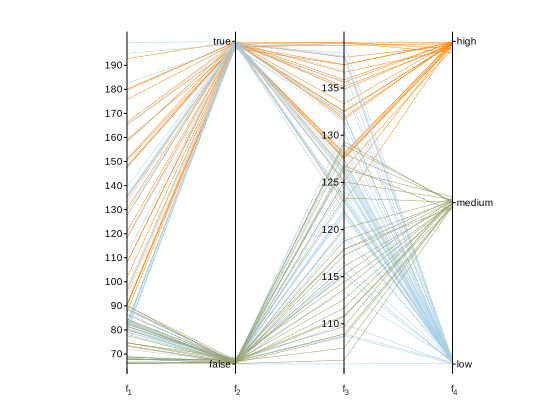
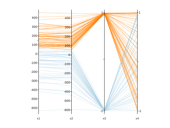
The function parallelplot creates a plot with Parallel Coordinates. In this type of plot, a parallel lines object stores an arbitrary set of axis objects to represent multi-dimensional data.
pie(x);
More Examples:
===! "Plot"
=== "C++"
```cpp
--8<-- "examples/data_distribution/pie/pie_1.cpp"
```
More Examples:
===! "Plot"
=== "C++"
```cpp
--8<-- "examples/data_distribution/pie/pie_2.cpp"
```
===! "Plot"
=== "C++"
```cpp
--8<-- "examples/data_distribution/pie/pie_3.cpp"
```
===! "Plot"
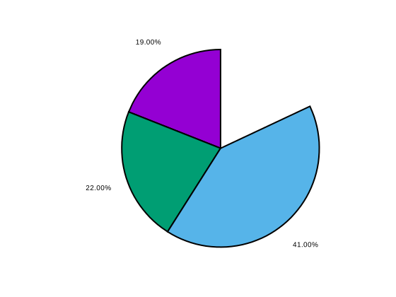
=== "C++"
```cpp
--8<-- "examples/data_distribution/pie/pie_4.cpp"
```
===! "Plot"
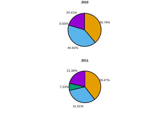
=== "C++"
```cpp
--8<-- "examples/data_distribution/pie/pie_5.cpp"
```
===! "Plot"
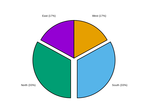
=== "C++"
```cpp
--8<-- "examples/data_distribution/pie/pie_6.cpp"
```
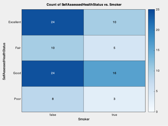
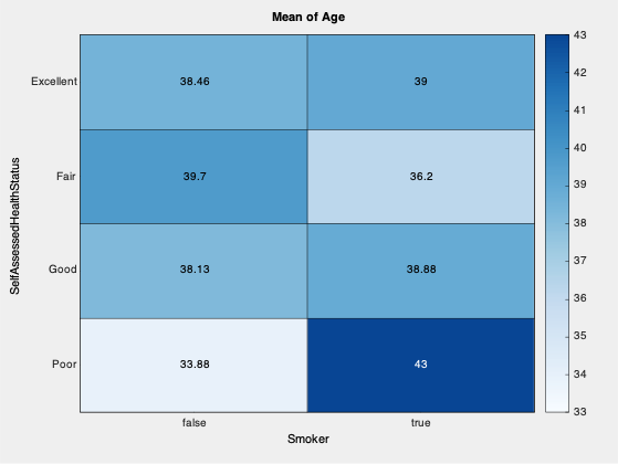
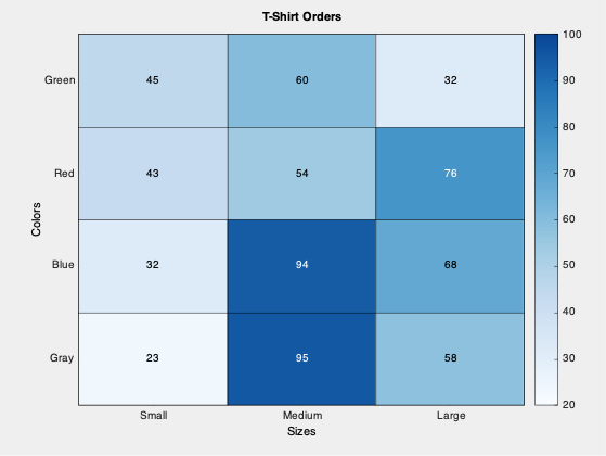
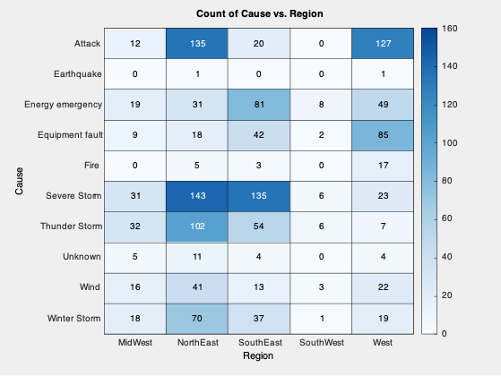
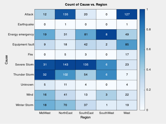
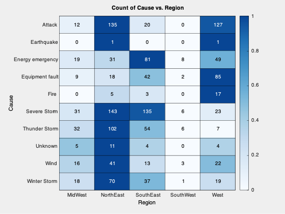
heatmap(data);
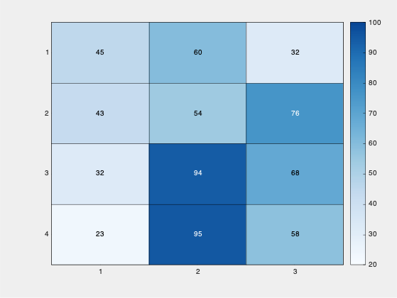
More Examples:
===! "Plot"
=== "C++"
```cpp
--8<-- "examples/data_distribution/heatmap/heatmap_1.cpp"
```
More Examples:
===! "Plot"
=== "C++"
```cpp
--8<-- "examples/data_distribution/heatmap/heatmap_2.cpp"
```
===! "Plot"
=== "C++"
```cpp
--8<-- "examples/data_distribution/heatmap/heatmap_3.cpp"
```
===! "Plot"
=== "C++"
```cpp
--8<-- "examples/data_distribution/heatmap/heatmap_4.cpp"
```
===! "Plot"
=== "C++"
```cpp
--8<-- "examples/data_distribution/heatmap/heatmap_5.cpp"
```
===! "Plot"
=== "C++"
```cpp
--8<-- "examples/data_distribution/heatmap/heatmap_6.cpp"
```
===! "Plot"
=== "C++"
```cpp
--8<-- "examples/data_distribution/heatmap/heatmap_7.cpp"
```
wordcloud(text, black_list);

More Examples:
===! "Plot"
=== "C++"
```cpp
--8<-- "examples/data_distribution/wordcloud/wordcloud_1.cpp"
```
More Examples:
===! "Plot"

=== "C++"
```cpp
--8<-- "examples/data_distribution/wordcloud/wordcloud_3.cpp"
```
===! "Plot"

=== "C++"
```cpp
--8<-- "examples/data_distribution/wordcloud/wordcloud_4.cpp"
```
===! "Plot"
=== "C++"
```cpp
--8<-- "examples/data_distribution/wordcloud/wordcloud_4.cpp"
```
Word clouds are generated from text or pairs of words and their frequency. After attributing a size proportional to each word frequency, the algorithm to position the labels iterates words from the largest to the smallest. For each word, it spins the word in polar coordinates converted to Cartesian coordinates until it does not overlap with any other word.
By default, the colors and the sizes depend on the word frequencies. We can customize the colors by passing a third parameter to the wordcloud function.
Bar Plot | Pareto Chart | Stem Plot | Stem Plot 3D
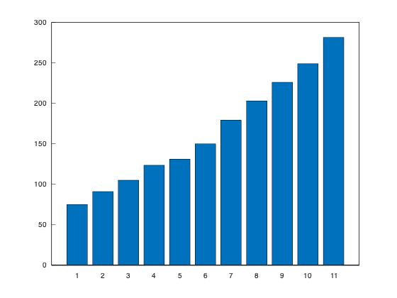
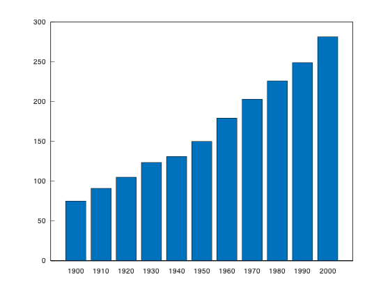
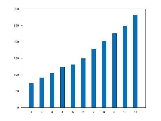
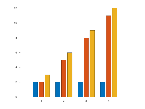
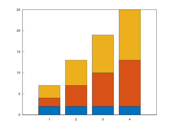
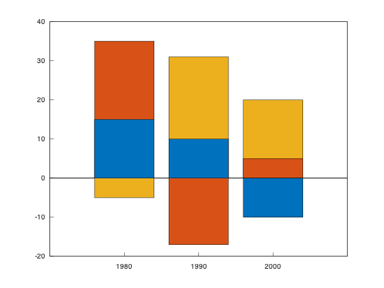
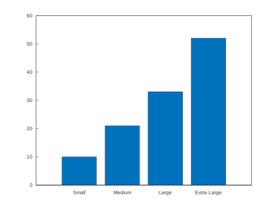
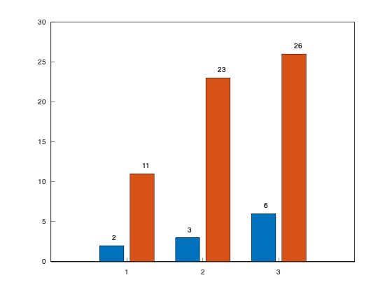
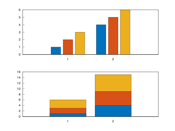
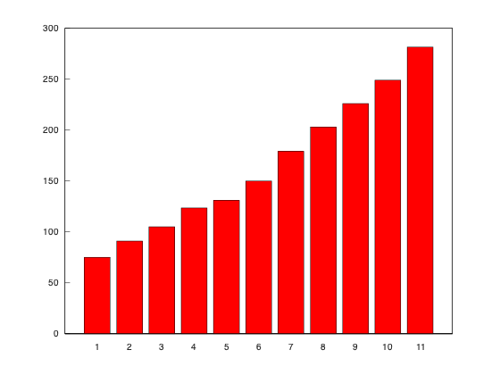
bar(y);
More Examples:
===! "Plot"
=== "C++"
```cpp
--8<-- "examples/discrete_data/bar/bar_1.cpp"
```
More Examples:
===! "Plot"
=== "C++"
```cpp
--8<-- "examples/discrete_data/bar/bar_2.cpp"
```
===! "Plot"
=== "C++"
```cpp
--8<-- "examples/discrete_data/bar/bar_3.cpp"
```
===! "Plot"
=== "C++"
```cpp
--8<-- "examples/discrete_data/bar/bar_4.cpp"
```
===! "Plot"
=== "C++"
```cpp
--8<-- "examples/discrete_data/bar/bar_5.cpp"
```
===! "Plot"
=== "C++"
```cpp
--8<-- "examples/discrete_data/bar/bar_6.cpp"
```
===! "Plot"
=== "C++"
```cpp
--8<-- "examples/discrete_data/bar/bar_7.cpp"
```
===! "Plot"
=== "C++"
```cpp
--8<-- "examples/discrete_data/bar/bar_8.cpp"
```
===! "Plot"
=== "C++"
```cpp
--8<-- "examples/discrete_data/bar/bar_9.cpp"
```
===! "Plot"
=== "C++"
```cpp
--8<-- "examples/discrete_data/bar/bar_10.cpp"
```
===! "Plot"
=== "C++"
```cpp
--8<-- "examples/discrete_data/bar/bar_11.cpp"
```
===! "Plot"
=== "C++"
```cpp
--8<-- "examples/discrete_data/bar/bar_12.cpp"
```
===! "Plot"
=== "C++"
```cpp
--8<-- "examples/discrete_data/bar/bar_13.cpp"
```
pareto(y);
More Examples:
===! "Plot"
=== "C++"
```cpp
--8<-- "examples/discrete_data/pareto/pareto_1.cpp"
```
More Examples:
===! "Plot"
=== "C++"
```cpp
--8<-- "examples/discrete_data/pareto/pareto_2.cpp"
```
===! "Plot"
=== "C++"
```cpp
--8<-- "examples/discrete_data/pareto/pareto_3.cpp"
```
===! "Plot"
=== "C++"
```cpp
--8<-- "examples/discrete_data/pareto/pareto_4.cpp"
```
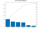
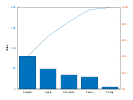
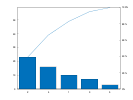
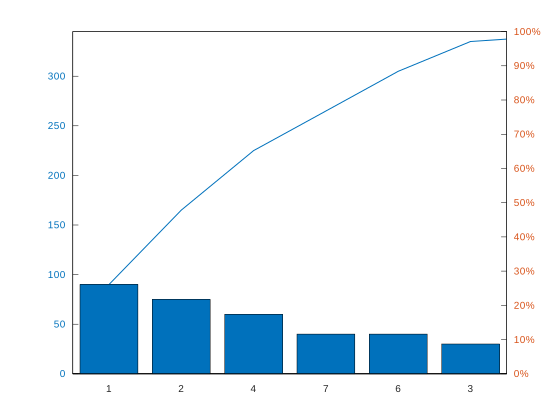
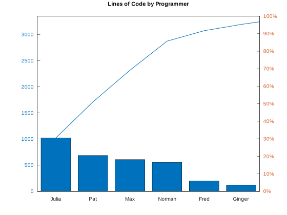
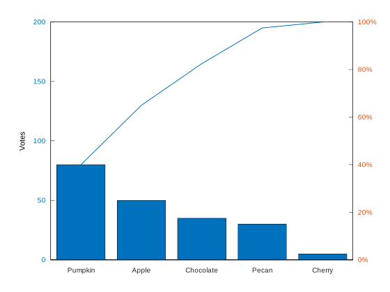
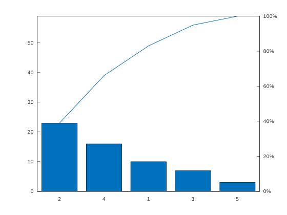
Pareto Charts are a type of chart that uses both axes. The
axis is used to represent bars with the data values in descending order. The
axis is used to represent the cumulative distribution function of the data in the
axis. By default, a Pareto Chart includes up to 10 items or as many items as needed to represent 95% of the cumulative distribution.
If you need Pareto fronts rather than Pareto charts, we refer to Scatter Plots for two-dimensional fronts, Plot matrices for three-dimensional fronts, or Parallel Coordinate Plots for many-objective fronts. These plot subcategories are described in Section Data Distribution. If you also need a tool to calculate these fronts efficiently, we refer to the Pareto Front Library.
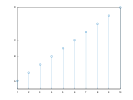
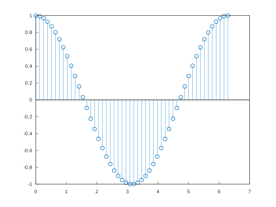
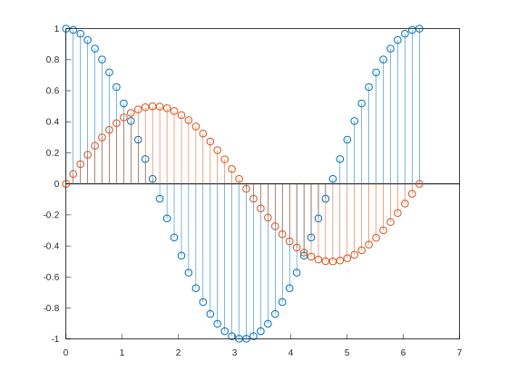
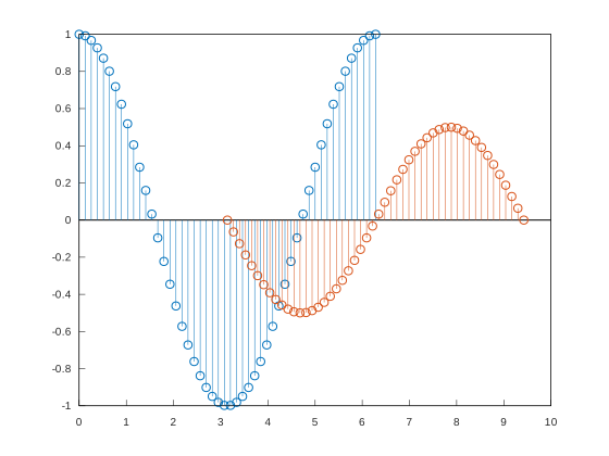
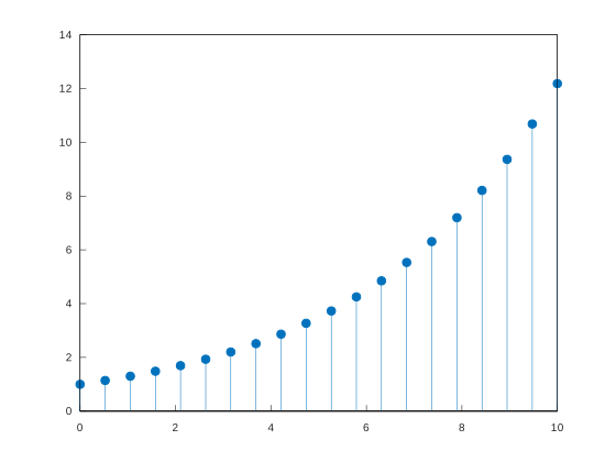
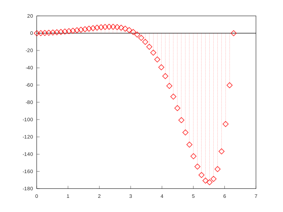
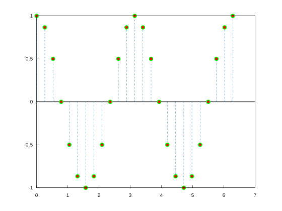
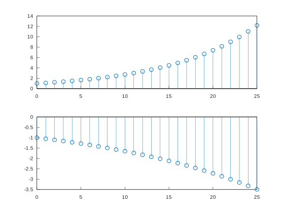
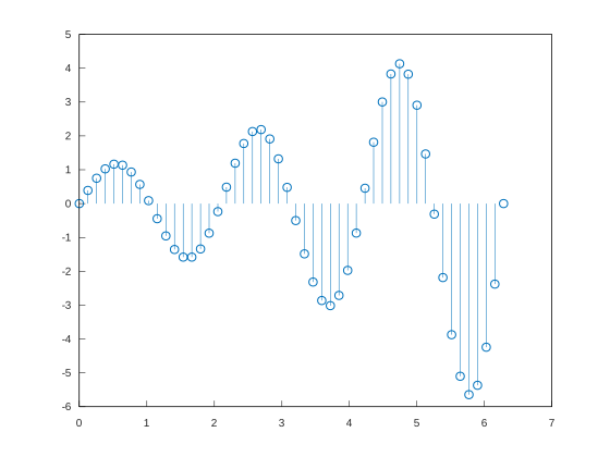
stem(Y);
More Examples:
===! "Plot"
=== "C++"
```cpp
--8<-- "examples/discrete_data/stem/stem_1.cpp"
```
More Examples:
===! "Plot"
=== "C++"
```cpp
--8<-- "examples/discrete_data/stem/stem_2.cpp"
```
===! "Plot"
=== "C++"
```cpp
--8<-- "examples/discrete_data/stem/stem_3.cpp"
```
===! "Plot"
=== "C++"
```cpp
--8<-- "examples/discrete_data/stem/stem_4.cpp"
```
===! "Plot"
=== "C++"
```cpp
--8<-- "examples/discrete_data/stem/stem_5.cpp"
```
===! "Plot"
=== "C++"
```cpp
--8<-- "examples/discrete_data/stem/stem_6.cpp"
```
===! "Plot"
=== "C++"
```cpp
--8<-- "examples/discrete_data/stem/stem_7.cpp"
```
===! "Plot"
=== "C++"
```cpp
--8<-- "examples/discrete_data/stem/stem_8.cpp"
```
===! "Plot"
=== "C++"
```cpp
--8<-- "examples/discrete_data/stem/stem_9.cpp"
```
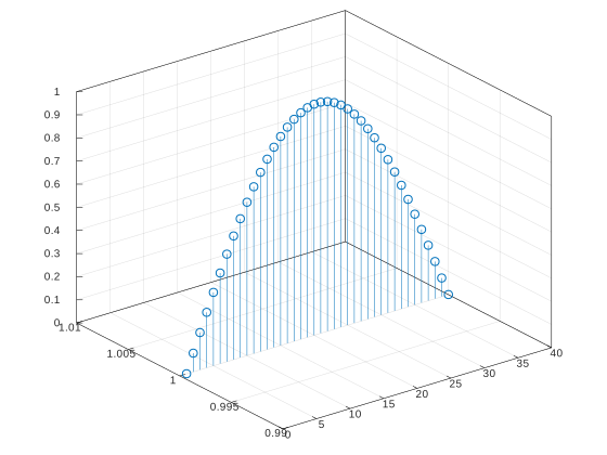
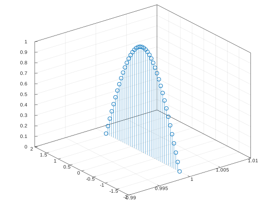
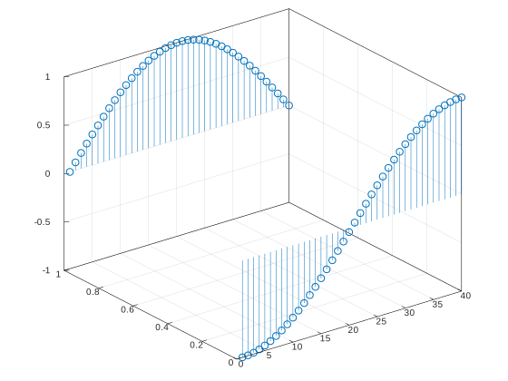
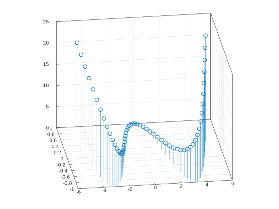
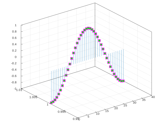
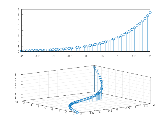
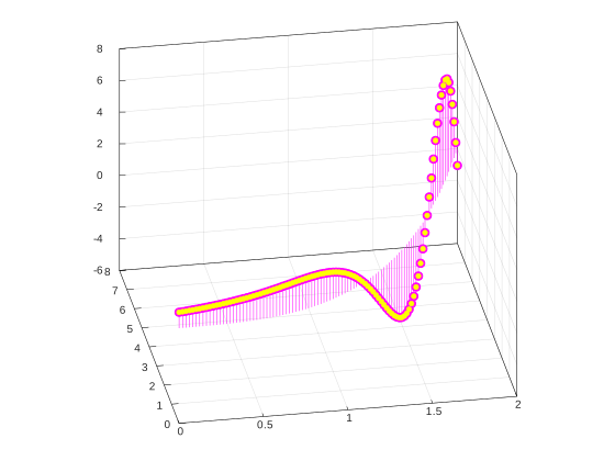
stem3(z);
More Examples:
===! "Plot"
=== "C++"
```cpp
--8<-- "examples/discrete_data/stem3/stem3_1.cpp"
```
More Examples:
===! "Plot"
=== "C++"
```cpp
--8<-- "examples/discrete_data/stem3/stem3_2.cpp"
```
===! "Plot"
=== "C++"
```cpp
--8<-- "examples/discrete_data/stem3/stem3_3.cpp"
```
===! "Plot"
=== "C++"
```cpp
--8<-- "examples/discrete_data/stem3/stem3_4.cpp"
```
===! "Plot"
=== "C++"
```cpp
--8<-- "examples/discrete_data/stem3/stem3_5.cpp"
```
===! "Plot"
=== "C++"
```cpp
--8<-- "examples/discrete_data/stem3/stem3_6.cpp"
```
===! "Plot"
=== "C++"
```cpp
--8<-- "examples/discrete_data/stem3/stem3_7.cpp"
```
===! "Plot"
=== "C++"
```cpp
--8<-- "examples/discrete_data/stem3/stem3_8.cpp"
```
===! "Plot"
=== "C++"
```cpp
--8<-- "examples/discrete_data/stem3/stem3_9.cpp"
```
===! "Plot"
=== "C++"
```cpp
--8<-- "examples/discrete_data/stem3/stem3_10.cpp"
```
===! "Plot"
=== "C++"
```cpp
--8<-- "examples/discrete_data/stem3/stem3_11.cpp"
```
Geoplot | Geoscatter Plot | Geobubble | Geodensity Plot
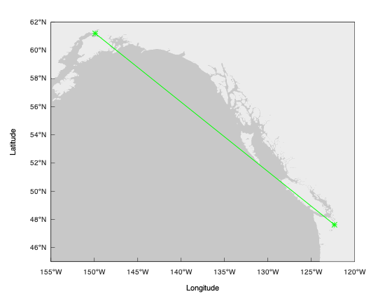
geoplot(lat,lon);
More Examples:
===! "Plot"
=== "C++"
```cpp
--8<-- "examples/geography/geoplot/geoplot_1.cpp"
```
More Examples:
===! "Plot"
=== "C++"
```cpp
--8<-- "examples/geography/geoplot/geoplot_2.cpp"
```
===! "Plot"
=== "C++"
```cpp
--8<-- "examples/geography/geoplot/geoplot_3.cpp"
```
===! "Plot"
=== "C++"
```cpp
--8<-- "examples/geography/geoplot/geoplot_4.cpp"
```
===! "Plot"
=== "C++"
```cpp
--8<-- "examples/geography/geoplot/geoplot_5.cpp"
```
===! "Plot"
=== "C++"
```cpp
--8<-- "examples/geography/geoplot/geoplot_6.cpp"
```
===! "Plot"
=== "C++"
```cpp
--8<-- "examples/geography/geoplot/geoplot_7.cpp"
```
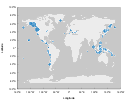
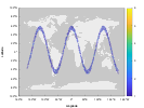
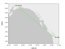
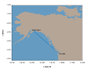
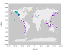
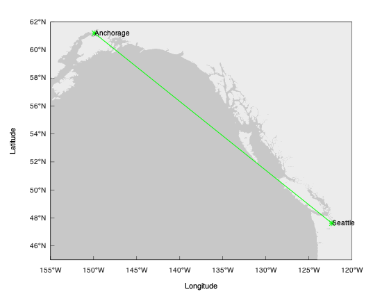
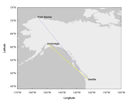
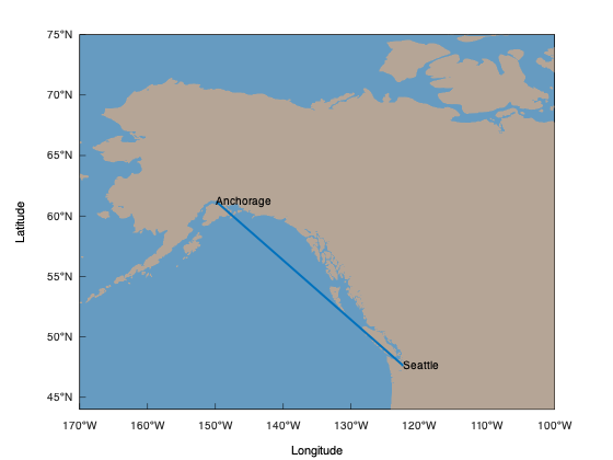
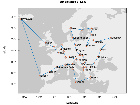
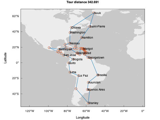
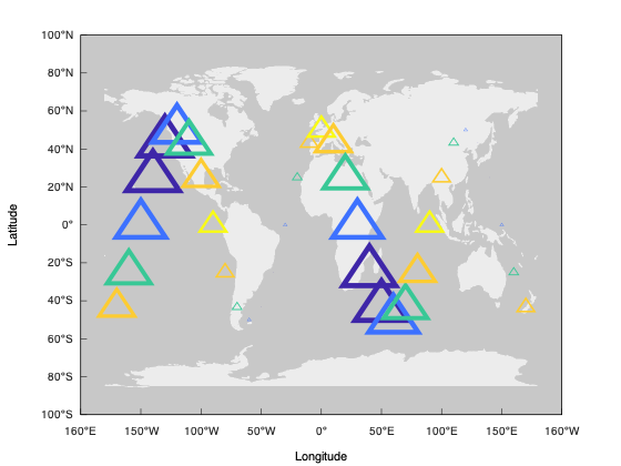
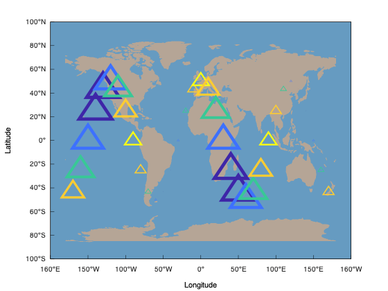
For the first geography plot, Matplot++ calls geoplot(), which creates a filled polygon with the world map. This first plot receives the tag "map" so that subsequent geography plots recognize there is no need to recreate this world map.
The data for the world map comes from Natural Earth. They provide data at 1:10m, 1:50m, and 1:110m scales. The geoplot function will initially use the data at the 1:110m scales. The geolimits function can be used to update the axis limits for geography plots. The difference between the usual functions for adjusting axis limits (xlim and ylim) and geolimits is that the latter will also update the map resolution according to the new limits for the and
axis.
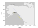
The geolimits function will query the figure size and, depending on the new limits for the axes, update the map to the 1:10m, or 1:50m scales if needed. Because it would be very inefficient to render the whole world map at a 1:10m or 1:50m scale only to display a region of this map, the geolimits function also crops the data pertinent to the new region being displayed.
Note that this does not only involve removing data points outside the new limits but it also needs to create new data points on the correct borders to create new polygons coherent with the map entry points in the region. For this reason, the algorithm needs to track all submaps represented as closed polygons in the original world map. If submaps are completely inside or outside the new ranges, we can respectively include or dismiss the data points. However, if the submap is only partially inside the new limits, to generate the correct borders for the polygons, we need to track all points outside the limits to classify the directions of these points outside the limits. We do that by only including points that change quadrants around the new limits so that the map entry points create polygons that look like they would if the complete world map were still being rendered outside these new limits.
If the you are not interested in geographic plots, the build script includes an option to remove the high-resolution maps at 1:10m and 1:50m scales from the library. In this case, the library will always use the map at a 1:110m scale no matter the axis limits.
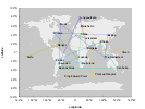
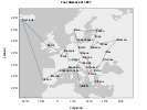
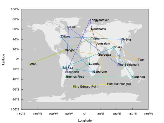
The function world_cities returns a list of major world cities. Its parameters define the minimum distances between cities in the and
axes. The
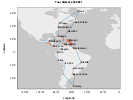
greedy_tsp function is a naive greedy algorithm to find a route between these cities as a Traveling Salesman Problem (TSP). We use the geoplot function to draw this route. Note that we use method chaining to define some further plot properties. Finally, the text function includes the city names in the map.
geoscatter(lat,lon);
More Examples:
===! "Plot"
=== "C++"
```cpp
--8<-- "examples/geography/geoscatter/geoscatter_1.cpp"
```
More Examples:
===! "Plot"
=== "C++"
```cpp
--8<-- "examples/geography/geoscatter/geoscatter_2.cpp"
```
geobubble(lat,lon,sizes);
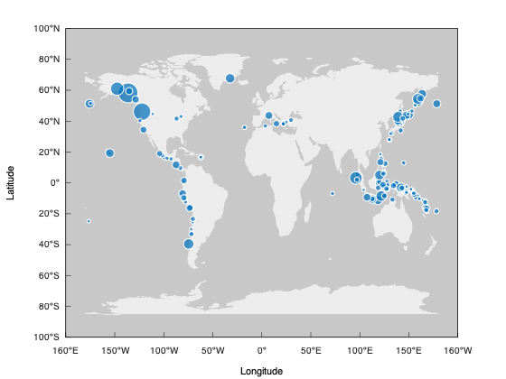
More Examples:
===! "Plot"
=== "C++"
```cpp
--8<-- "examples/geography/geobubble/geobubble_1.cpp"
```
More Examples:
===! "Plot"
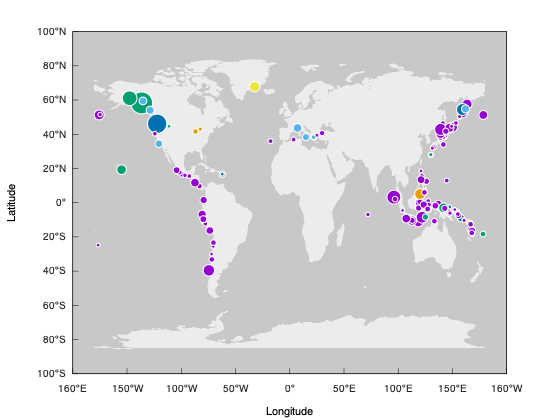
=== "C++"
```cpp
--8<-- "examples/geography/geobubble/geobubble_2.cpp"
```
geodensityplot(lat, lon);
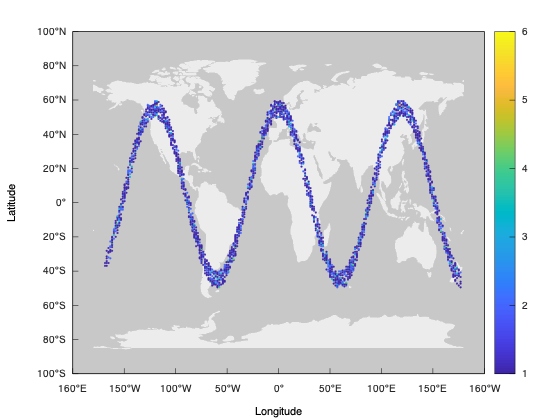
=== "Plot"
=== "C++"
```cpp
--8<-- "examples/geography/geodensityplot/geodensityplot_1.cpp"
```
Polar Line Plot | Polar Scatter Plot | Polar Histogram | Compass | Polar Function
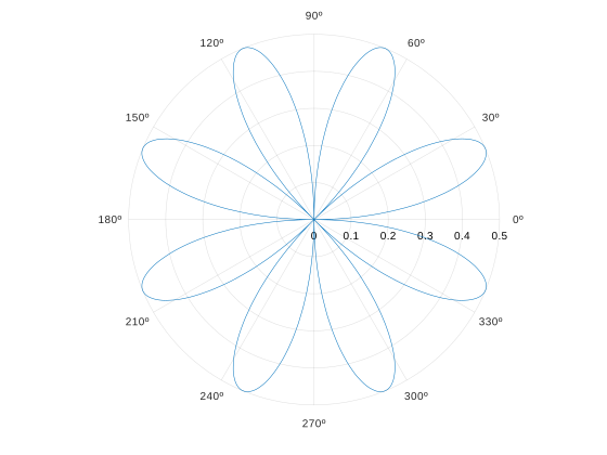
polarplot(theta, rho);
More Examples:
===! "Plot"
=== "C++"
```cpp
--8<-- "examples/polar_plots/polarplot/polarplot_1.cpp"
```
More Examples:
===! "Plot"
=== "C++"
```cpp
--8<-- "examples/polar_plots/polarplot/polarplot_2.cpp"
```
===! "Plot"
=== "C++"
```cpp
--8<-- "examples/polar_plots/polarplot/polarplot_3.cpp"
```
===! "Plot"
=== "C++"
```cpp
--8<-- "examples/polar_plots/polarplot/polarplot_4.cpp"
```
===! "Plot"
=== "C++"
```cpp
--8<-- "examples/polar_plots/polarplot/polarplot_5.cpp"
```
===! "Plot"
=== "C++"
```cpp
--8<-- "examples/polar_plots/polarplot/polarplot_6.cpp"
```
===! "Plot"
=== "C++"
```cpp
--8<-- "examples/polar_plots/polarplot/polarplot_7.cpp"
```
===! "Plot"
=== "C++"
```cpp
--8<-- "examples/polar_plots/polarplot/polarplot_8.cpp"
```
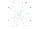
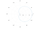
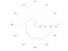
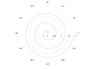
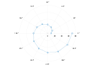
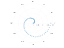
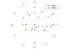
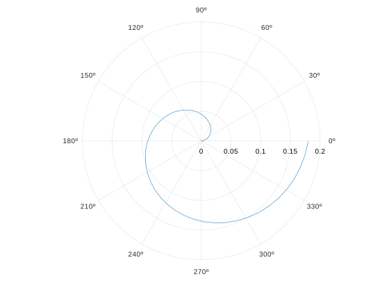
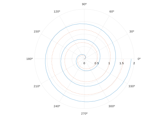
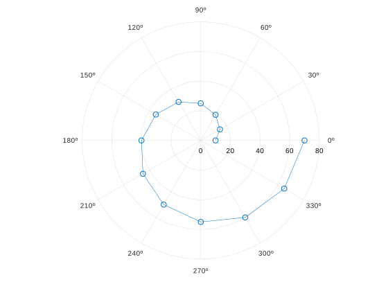
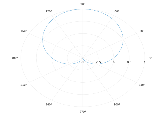
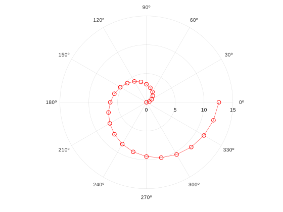
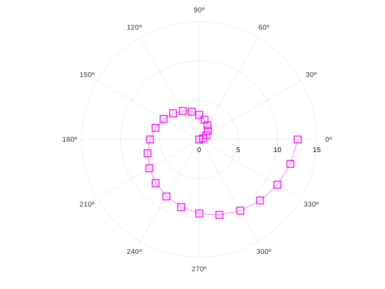
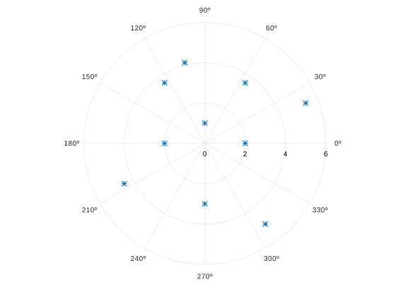
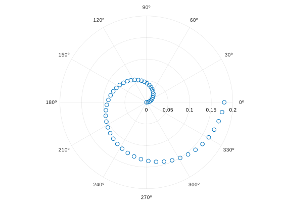
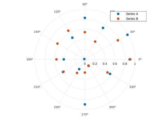
By emplacing a polar plot in the axes, the axes move to a polar mode, where we use the and
axis instead of the
and
axis.
From the backend point of view, these axes are an abstraction to the user. The data points in the and
axis are drawn by converting the positions from the polar coordinates
and
to the Cartesian coordinates
and
with the relationships
and
.
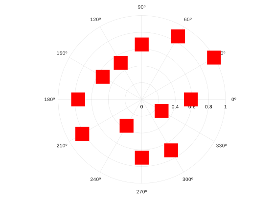
Aside from this conversion, these plot subcategories are analogous to line plots, scatter plots, histograms, quiver plots, and line functions.
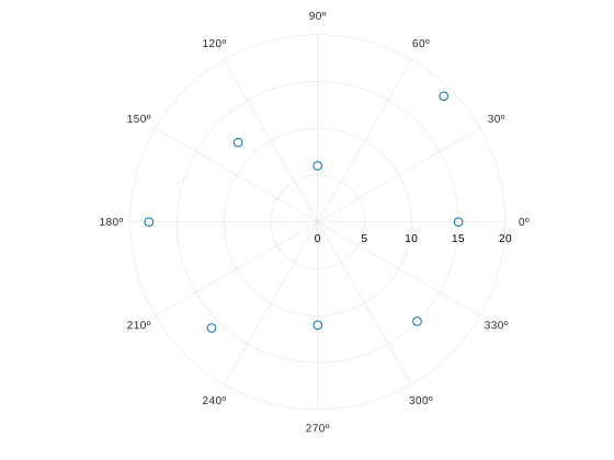
polarscatter(theta, rho);
More Examples:
===! "Plot"
=== "C++"
```cpp
--8<-- "examples/polar_plots/polarscatter/polarscatter_1.cpp"
```
More Examples:
===! "Plot"
=== "C++"
```cpp
--8<-- "examples/polar_plots/polarscatter/polarscatter_2.cpp"
```
===! "Plot"
=== "C++"
```cpp
--8<-- "examples/polar_plots/polarscatter/polarscatter_3.cpp"
```
===! "Plot"
=== "C++"
```cpp
--8<-- "examples/polar_plots/polarscatter/polarscatter_4.cpp"
```
===! "Plot"
=== "C++"
```cpp
--8<-- "examples/polar_plots/polarscatter/polarscatter_5.cpp"
```
===! "Plot"
=== "C++"
```cpp
--8<-- "examples/polar_plots/polarscatter/polarscatter_6.cpp"
```
polarhistogram(theta, 6);
More Examples:
===! "Plot"
=== "C++"
```cpp
--8<-- "examples/polar_plots/polarhistogram/polarhistogram_1.cpp"
```
More Examples:
===! "Plot"
=== "C++"
```cpp
--8<-- "examples/polar_plots/polarhistogram/polarhistogram_2.cpp"
```
===! "Plot"
=== "C++"
```cpp
--8<-- "examples/polar_plots/polarhistogram/polarhistogram_3.cpp"
```
===! "Plot"
=== "C++"
```cpp
--8<-- "examples/polar_plots/polarhistogram/polarhistogram_4.cpp"
```
===! "Plot"
=== "C++"
```cpp
--8<-- "examples/polar_plots/polarhistogram/polarhistogram_5.cpp"
```
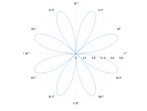
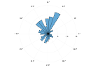
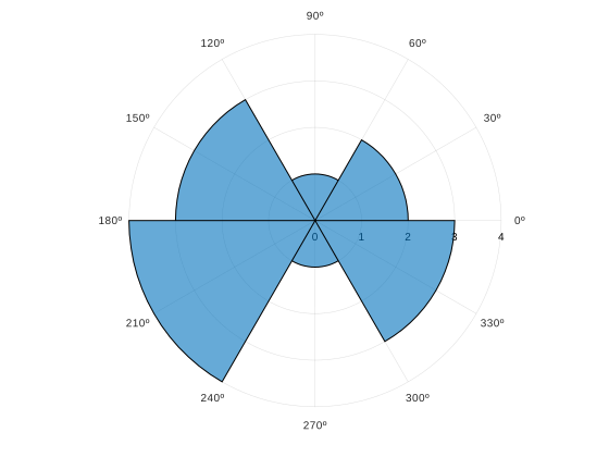
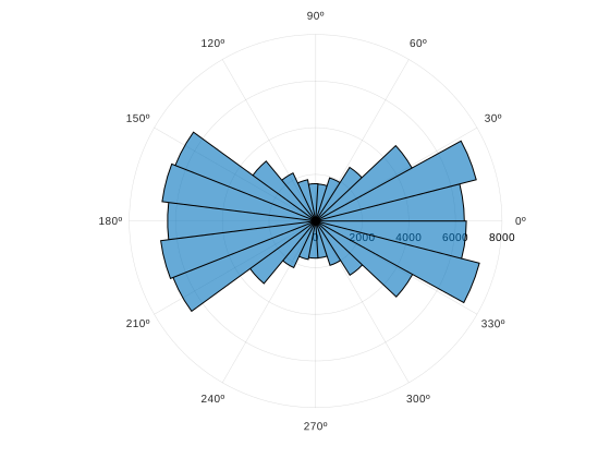
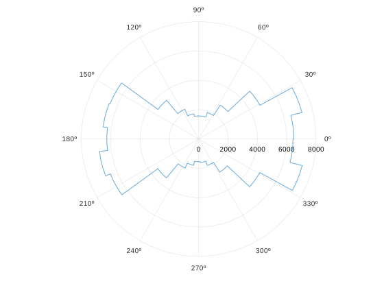
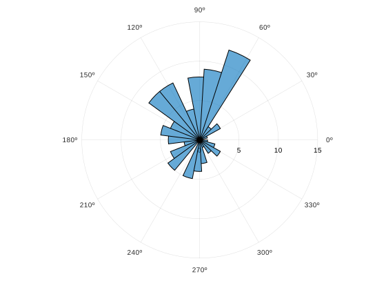
The function polarhistogram distributes the data into the number of bins provided as its second parameter.
compass(u, v);

More Examples:
===! "Plot"
=== "C++"
```cpp
--8<-- "examples/polar_plots/compass/compass_1.cpp"
```
More Examples:
===! "Plot"
=== "C++"
```cpp
--8<-- "examples/polar_plots/compass/compass_2.cpp"
```
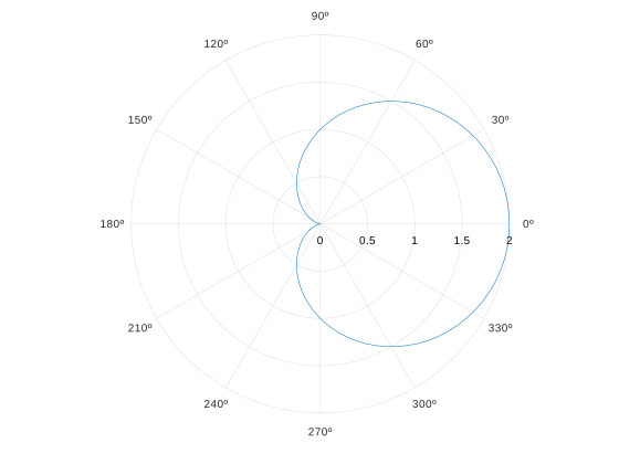
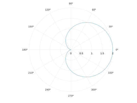
ezpolar(fn);
More Examples:
===! "Plot"
=== "C++"
```cpp
--8<-- "examples/polar_plots/ezpolar/ezpolar_1.cpp"
```
More Examples:
===! "Plot"
=== "C++"
```cpp
--8<-- "examples/polar_plots/ezpolar/ezpolar_2.cpp"
```
Contour | Filled Contour | Function Contour
contour(X, Y, Z);
More Examples:
===! "Plot"
=== "C++"
```cpp
--8<-- "examples/contour_plots/contour/contour_1.cpp"
```
More Examples:
===! "Plot"
=== "C++"
```cpp
--8<-- "examples/contour_plots/contour/contour_2.cpp"
```
===! "Plot"
=== "C++"
```cpp
--8<-- "examples/contour_plots/contour/contour_3.cpp"
```
===! "Plot"
=== "C++"
```cpp
--8<-- "examples/contour_plots/contour/contour_4.cpp"
```
===! "Plot"
=== "C++"
```cpp
--8<-- "examples/contour_plots/contour/contour_5.cpp"
```
===! "Plot"
=== "C++"
```cpp
--8<-- "examples/contour_plots/contour/contour_6.cpp"
```
===! "Plot"
=== "C++"
```cpp
--8<-- "examples/contour_plots/contour/contour_7.cpp"
```
===! "Plot"
=== "C++"
```cpp
--8<-- "examples/contour_plots/contour/contour_8.cpp"
```
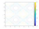
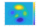
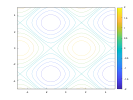
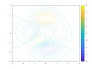
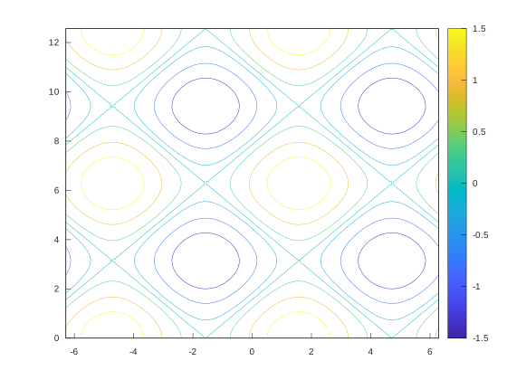
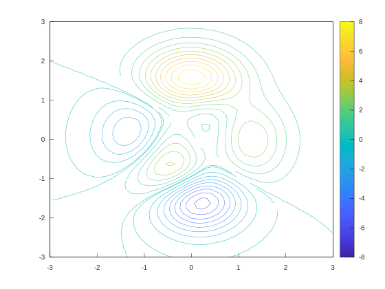
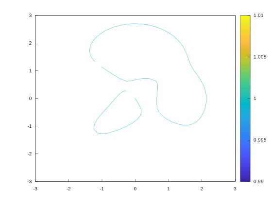
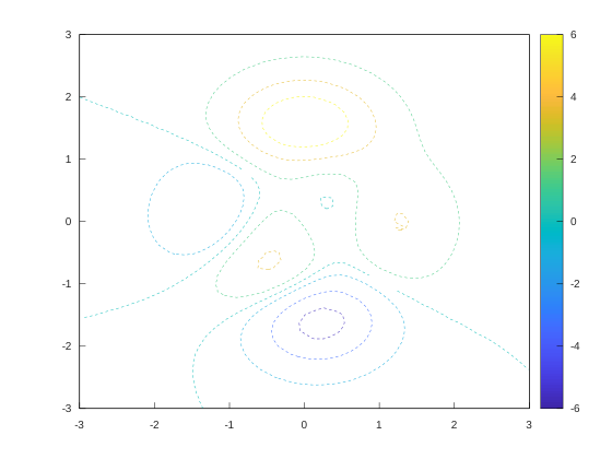
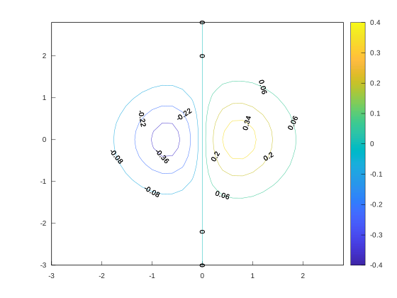
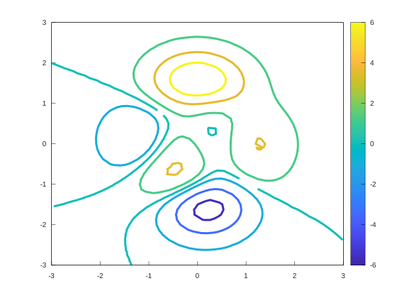
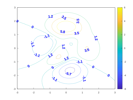
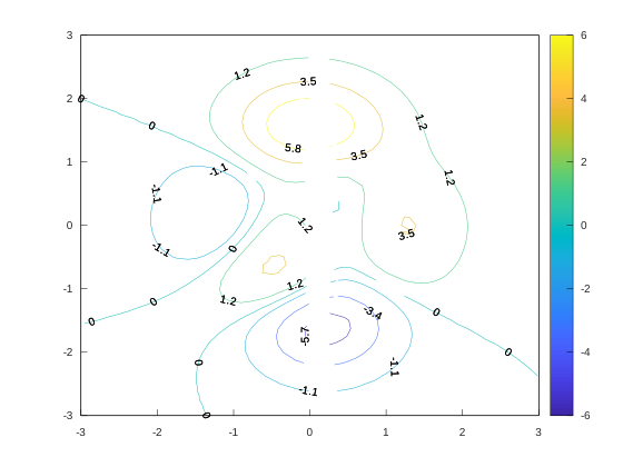
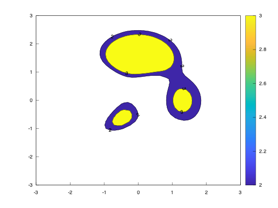
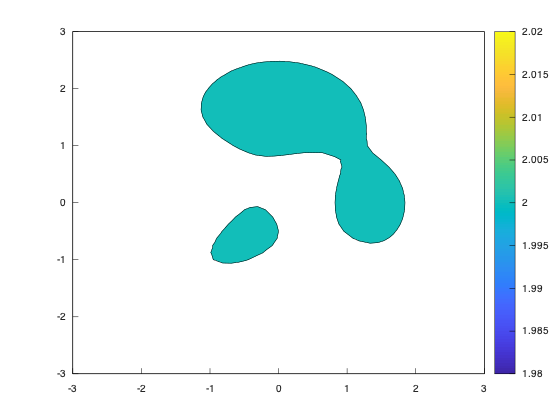
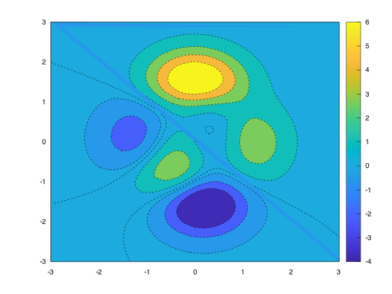
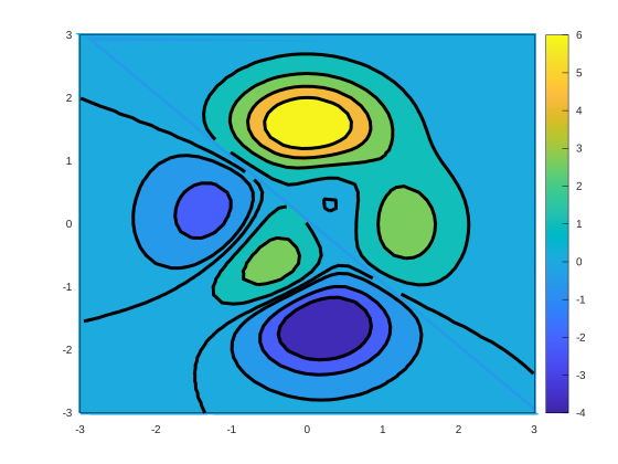
All these subcategories depend on the contours type. They also depend on lazy evaluation for generating the contour lines. When the function draw is called in the contours class, it preprocesses all contour lines for a three-dimensional function.
Although it is relatively simple to show a heatmap with the values for the -axis, calculating contour lines relative to the
-axis is more complex than it might seem at first. We provide the function
contourc for calculating contour lines. This function uses an adaptation of the algorithm adopted by Matplotlib.
The algorithm creates a quad grid defined by the and
values. It uses this grid to infer a contour line passing through positions with the same
value. The algorithm sweeps through the grid twice to generate these lines. The first sweep looks for lines that start on the boundaries. The second sweep looks for interior closed loops.
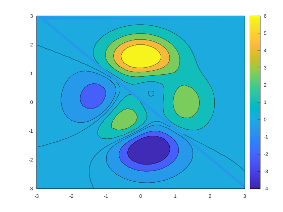
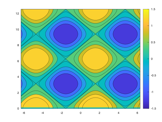
Filled contours are closed polygons for pairs of contour levels. Some polygons for filled contours might be holes inside other polygons. The algorithm needs to keep track of these relationships so that we can render the polygons in their accurate order. To avoid an extra step that identifies this relationship between the polygons, the sweeping algorithm already identifies which polygons are holes for each level.
Once we find the quads with the contour line, the line is generated by interpolating the values around that quad.
contourf(X, Y, Z);
More Examples:
===! "Plot"
=== "C++"
```cpp
--8<-- "examples/contour_plots/contourf/contourf_1.cpp"
```
More Examples:
===! "Plot"
=== "C++"
```cpp
--8<-- "examples/contour_plots/contourf/contourf_2.cpp"
```
===! "Plot"
=== "C++"
```cpp
--8<-- "examples/contour_plots/contourf/contourf_3.cpp"
```
===! "Plot"
=== "C++"
```cpp
--8<-- "examples/contour_plots/contourf/contourf_4.cpp"
```
===! "Plot"
=== "C++"
```cpp
--8<-- "examples/contour_plots/contourf/contourf_5.cpp"
```
===! "Plot"
=== "C++"
```cpp
--8<-- "examples/contour_plots/contourf/contourf_6.cpp"
```
fcontour(f);
More Examples:
===! "Plot"
=== "C++"
```cpp
--8<-- "examples/contour_plots/fcontour/fcontour_1.cpp"
```
More Examples:
===! "Plot"
=== "C++"
```cpp
--8<-- "examples/contour_plots/fcontour/fcontour_2.cpp"
```
===! "Plot"
=== "C++"
```cpp
--8<-- "examples/contour_plots/fcontour/fcontour_3.cpp"
```
===! "Plot"
=== "C++"
```cpp
--8<-- "examples/contour_plots/fcontour/fcontour_4.cpp"
```
===! "Plot"
=== "C++"
```cpp
--8<-- "examples/contour_plots/fcontour/fcontour_5.cpp"
```
===! "Plot"
=== "C++"
```cpp
--8<-- "examples/contour_plots/fcontour/fcontour_6.cpp"
```
===! "Plot"
=== "C++"
```cpp
--8<-- "examples/contour_plots/fcontour/fcontour_7.cpp"
```
===! "Plot"
=== "C++"
```cpp
--8<-- "examples/contour_plots/fcontour/fcontour_8.cpp"
```
===! "Plot"
=== "C++"
```cpp
--8<-- "examples/contour_plots/fcontour/fcontour_9.cpp"
```
===! "Plot"
=== "C++"
```cpp
--8<-- "examples/contour_plots/fcontour/fcontour_10.cpp"
```
===! "Plot"
=== "C++"
```cpp
--8<-- "examples/contour_plots/fcontour/fcontour_11.cpp"
```
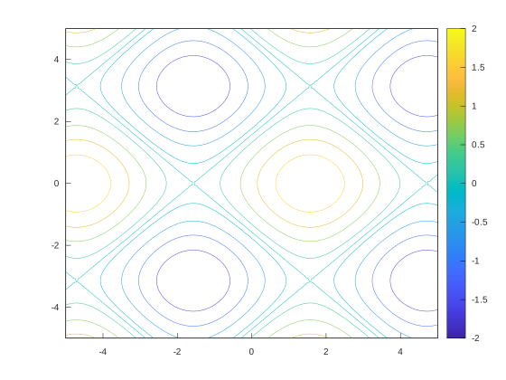
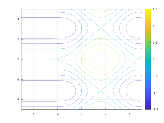
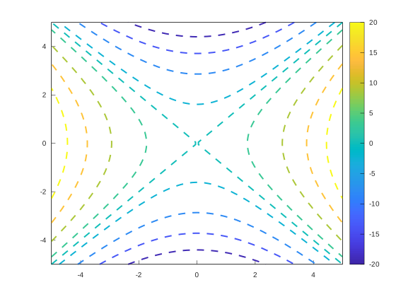
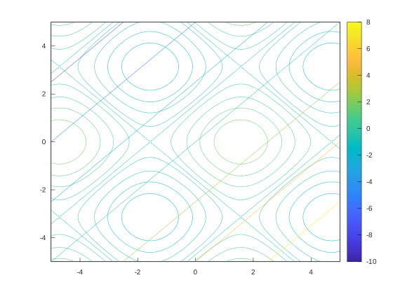
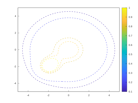
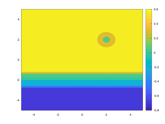
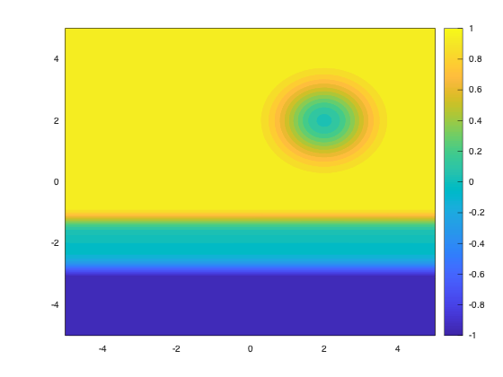
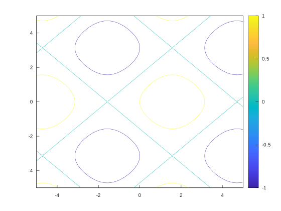
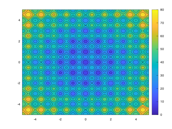
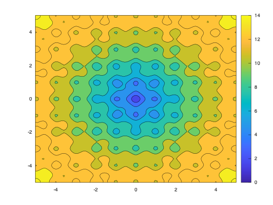
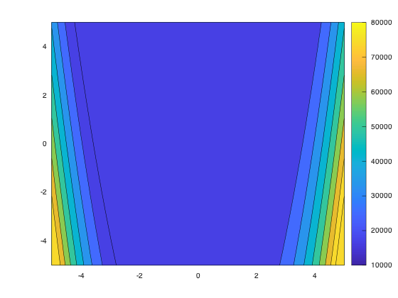
By default, the function fcontour will generate 9 contour lines from a lambda function. The functions contour and contourf, on the other hand, plot contour lines and filled contour lines from a grid of data points for ,
, and
.
quiver(x, y, u, v);
More Examples:
===! "Plot"
=== "C++"
```cpp
--8<-- "examples/vector_fields/quiver/quiver_1.cpp"
```
More Examples:
===! "Plot"
=== "C++"
```cpp
--8<-- "examples/vector_fields/quiver/quiver_2.cpp"
```
===! "Plot"
=== "C++"
```cpp
--8<-- "examples/vector_fields/quiver/quiver_3.cpp"
```
===! "Plot"
=== "C++"
```cpp
--8<-- "examples/vector_fields/quiver/quiver_4.cpp"
```
===! "Plot"
=== "C++"
```cpp
--8<-- "examples/vector_fields/quiver/quiver_6.cpp"
```
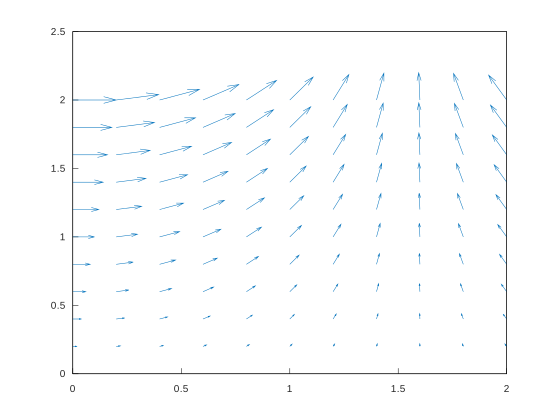
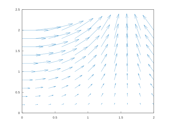
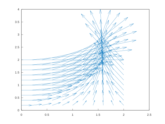
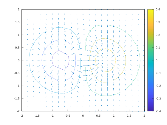
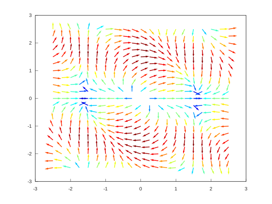
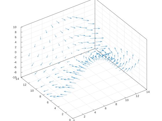
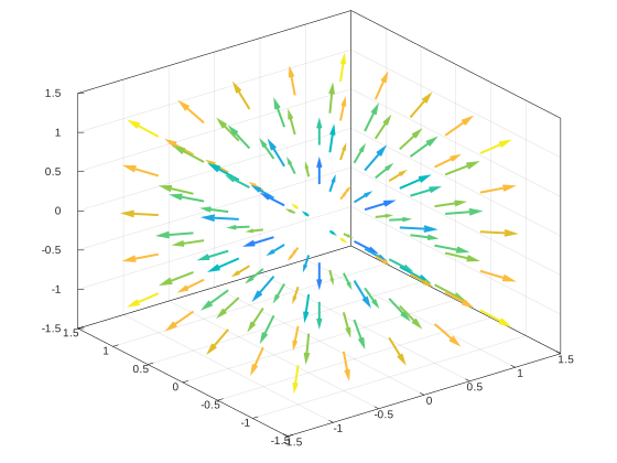
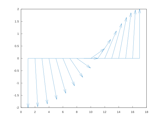
All these subcategories depend on the vectors object type. In a two-dimensional plot, for each value of and
with the position of a vector, it also requires the value of
and
indicating its direction and magnitude. In a three-dimensional plot, the direction and magnitude are defined by
,
, and
.
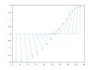
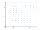
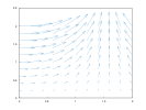
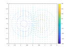
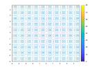
A quiver plot (or velocity plot) shows a grid of vectors whose direction and magnitude are scaled to prevent the overlap between vectors in subsequent quads.
quiver3(Z, U, V, W);
===! "Plot"
=== "C++"
```cpp
--8<-- "examples/vector_fields/quiver3/quiver3_1.cpp"
```
===! "Plot"
=== "C++"
```cpp
--8<-- "examples/vector_fields/quiver3/quiver3_2.cpp"
```
feather(u, v);
===! "Plot"
=== "C++"
```cpp
--8<-- "examples/vector_fields/feather/feather_1.cpp"
```
Surface | Surface with Contour | Mesh | Mesh with Contour | Mesh with Curtain | Function Surface | Function Mesh | Waterfall | Fence | Ribbon
surf(X, Y, Z);
More Examples:
===! "Plot"
=== "C++"
```cpp
--8<-- "examples/surfaces/surf/surf_1.cpp"
```
More Examples:
===! "Plot"
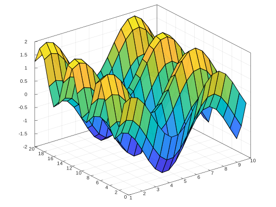
=== "C++"
```cpp
--8<-- "examples/surfaces/surf/surf_2.cpp"
```
===! "Plot"
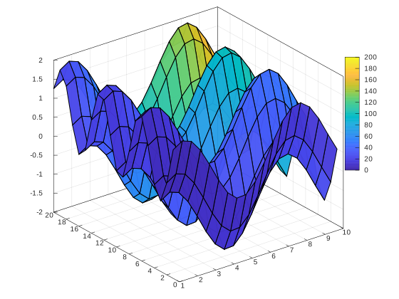
=== "C++"
```cpp
--8<-- "examples/surfaces/surf/surf_3.cpp"
```
===! "Plot"
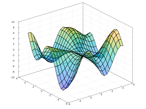
=== "C++"
```cpp
--8<-- "examples/surfaces/surf/surf_4.cpp"
```
===! "Plot"
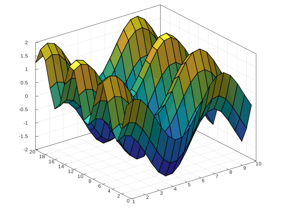
=== "C++"
```cpp
--8<-- "examples/surfaces/surf/surf_5.cpp"
```
===! "Plot"
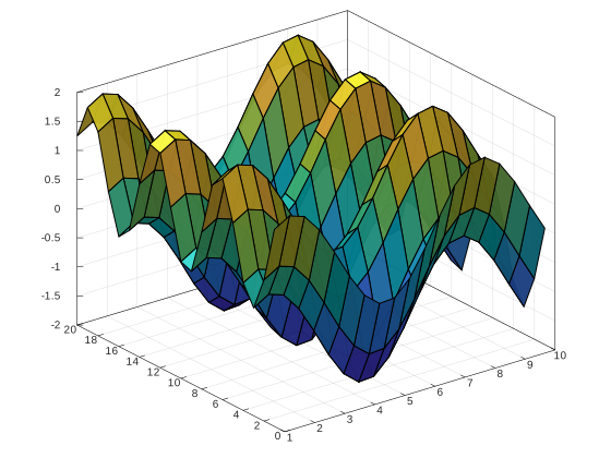
=== "C++"
```cpp
--8<-- "examples/surfaces/surf/surf_6.cpp"
```
Truncated — view the full README on GitHub.
(top 24 of 41)
936 followers · starred Aug 2020
207 followers · starred Aug 2020
85 followers · starred Jun 2024
81 followers · starred Aug 2020
Matplot++: A C++ Graphics Library for Data Visualization 📊🗾
See the codeA C++ Graphics Library for Data Visualization
Data visualization can help programmers and scientists identify trends in their data and efficiently communicate these results with their peers. Modern C++ is being used for a variety of scientific applications, and this environment can benefit considerably from graphics libraries that attend the typical design goals toward scientific data visualization. Besides the option of exporting results to other environments, the customary alternatives in C++ are either non-dedicated libraries that depend on existing user interfaces or bindings to other languages. Matplot++ is a graphics library for data visualization that provides interactive plotting, means for exporting plots in high-quality formats for scientific publications, a compact syntax consistent with similar libraries, dozens of plot categories with specialized algorithms, multiple coding styles, and supports generic backends.
READ THE DOCUMENTATION FOR A QUICK START AND EXAMPLES
Vcpkg users can install Matplot++ with the matplotplusplus port:
vcpkg install matplotplusplus
This formula is a contribution to vcpkg by @myd7349.
Mac users can install Matplot++ with Homebrew:
brew install matplotplusplus
This formula is a contribution to Homebrew by Andrew Kane.
Matplot++ is available in the Arch User Repository
(AUR) as
matplotplusplus.
Note you can manually install the package by following the instructions on the
Arch Wiki
or use an AUR helper like
yay
(recommended for ease of install).
yay -S matplotplusplus
To discuss any issues related to this package refer to the comments section on
the AUR page of matplotplusplus here.
You can use Matplot++ directly in CMake projects as a subproject, without installing it. This is convenient if you are experimenting with this library for the first time or don't expect your users to have Matplot++ installed on their systems.
Check if you have Cmake 3.14+ installed:
cmake --version
Clone the whole project
git clone https://github.com/alandefreitas/matplotplusplus/
and add the subdirectory to your CMake project:
add_subdirectory(matplotplusplus)
When creating your executable, link the library to the targets you want:
add_executable(my_target main.cpp)
target_link_libraries(my_target PUBLIC matplot)
Add this header to your source files:
#include <matplot/matplot.h>
However, in larger projects, it's always recommended to look for Matplot++ with find_package before including it as a subdirectory to avoid ODR errors.
If you have CMake 3.21 or greater, you can use the system build preset to
build the package system-wide:
cmake --preset=system
cmake --build --preset=system
sudo cmake --install build/system
Alternatively, if the CMAKE_PREFIX_PATH environment variable is set to
$HOME/.local, then you can install it locally. This can be set in /etc/profile
or your shell config. This will not affect discovery of packages installed
system-wide.
export CMAKE_PREFIX_PATH="$HOME/.local"
This has the advantage of not
requiring sudo, and matplotplusplus will be installed in $HOME/.local.
cmake --preset=local
cmake --build --preset=local
cmake --install build/local
You can now use it from CMake with find_package:
find_package(Matplot++ REQUIRED)
target_link_libraries(<your target> Matplot++::matplot)
If you're using a version of CMake too old to support presets, then building with the system preset is equivilant to:
cmake -B build/system \
-DMATPLOTPP_BUILD_EXAMPLES=OFF \
-DMATPLOTPP_BUILD_SHARED_LIBS=ON \
-DMATPLOTPP_BUILD_TESTS=OFF \
-DCMAKE_BUILD_TYPE=Release \
-DCMAKE_INTERPROCEDURAL_OPTIMIZATION=ON
cmake --build build/system
While building with the local preset is equivilant to:
cmake -B build/local \
-DMATPLOTPP_BUILD_EXAMPLES=OFF \
-DMATPLOTPP_BUILD_SHARED_LIBS=ON \
-DMATPLOTPP_BUILD_TESTS=OFF \
-DCMAKE_BUILD_TYPE=Release \
-DCMAKE_INSTALL_PREFIX="$HOME/.local" \
-DCMAKE_INTERPROCEDURAL_OPTIMIZATION=ON
cmake --build build/local
FetchContent is a CMake command that can automatically download the Matplot++ repository. Check if you have Cmake 3.14+ installed:
cmake --version
Include FetchContent in your CMake build script:
include(FetchContent)
Declare the source for the contents:
FetchContent_Declare(matplotplusplus
GIT_REPOSITORY https://github.com/alandefreitas/matplotplusplus
GIT_TAG origin/master) # or whatever tag you want
Let CMake download the repository and include it as a subdirectory.
FetchContent_GetProperties(matplotplusplus)
if(NOT matplotplusplus_POPULATED)
FetchContent_Populate(matplotplusplus)
add_subdirectory(${matplotplusplus_SOURCE_DIR} ${matplotplusplus_BINARY_DIR} EXCLUDE_FROM_ALL)
endif()
When creating your executable, link the library to the targets you want:
add_executable(my_target main.cpp)
target_link_libraries(my_target PUBLIC matplot)
Then add this header to your source files:
#include <matplot/matplot.h>
However, in larger projects, it's always recommended to look for Matplot++ with find_package before including it as a subdirectory to avoid ODR errors.
CPM.cmake is a nice wrapper around the CMake FetchContent function.
Check if you have Cmake 3.14+ installed:
cmake --version
Install CPM.cmake and then use this command to add Matplot++ to your build script:
CPMAddPackage(
NAME matplotplusplus
GITHUB_REPOSITORY alandefreitas/matplotplusplus
GIT_TAG origin/master # or whatever tag you want
)
# ...
target_link_libraries(my_target PUBLIC matplot)
Then add this header to your source files:
#include <matplot/matplot.h>
However, in larger projects, it's always recommended to look for Matplot++ with find_package before including it as a subdirectory to avoid ODR errors.
You can use:
option(CPM_USE_LOCAL_PACKAGES "Try `find_package` before downloading dependencies" ON)
in your build script to let CPM.cmake do that for you.
If you have the library installed on your system, you can call find_package() from your CMake build script.
find_package(Matplot++ REQUIRED)
When creating your executable, link the library to the targets you want:
add_executable(my_target main.cpp)
target_link_libraries(my_target PUBLIC Matplot++::matplot)
Then add this header to your source files:
#include <matplot/matplot.h>
You can see a complete example in test/integration/CMakeLists.txt.
CMake should be able to locate the Matplot++Config.cmake script automatically if you installed the library under /usr/local/ (Linux / Mac OS). Unfortunately, there is no easy default directory for find_package on Windows.
!!! warning "Default directories"
By default, the library is likely to be in `/usr/local/` (Linux / Mac OS) or `C:/Program Files/` (Windows). The installer will try to find the directory where you usually keep your libraries but that's not always perfect.
!!! warning "Finding packages on Windows"
Unfortunately, CMake does not have a single default directory for packages on Windows like `/usr/local/lib`. If CMake cannot find Matplot++ on Windows or if you installed the library outside the default directory on Linux/Mac OS, there are a few [options](https://stackoverflow.com/questions/21314893/what-is-the-default-search-path-for-find-package-in-windows-using-cmake):
* **Environment Variables**: The most reliable way to set this default directory is through environment variables. You can create an environment variable `MATPLOTPP_DIR` and then add `$ENV{MATPLOTPP_DIR}` to the `HINTS` section of the `find_package` command. This tends to be more convenient than requiring the path on the command line every time. Starting with version 3.12, CMake now implicitly considers the `<PackageName>_Root` environment variable a HINT for every `find_package` call.
* **Package Registry**: CMake offers the [Package Registry](https://cmake.org/cmake/help/v3.5/manual/cmake-packages.7.html#package-registry) as an alternative mechanism for finding package locations. CMake maintains a list of package information in the Windows registry under `HKEY_CURRENT_USER\Software\Kitware\CMake\Packages\`.
* **Append CMAKE_MODULE_PATH**: You can append more directories to [`CMAKE_MODULE_PATH`](https://cmake.org/cmake/help/latest/variable/CMAKE_MODULE_PATH.html) with something like `list(APPEND CMAKE_MODULE_PATH "C:\\Program Files\\matplotplusplus 1.0.1")`. `CMAKE_MODULE_PATH` is a list of search paths for CMake modules to be loaded by the `include()` or `find_package()` commands.
* **Set the DIR variable directly**: Directly set the `Matplot++_DIR` variable with something like `set(Matplot++_DIR "C:\\Program Files\\matplotplusplus 1.0.1\\lib\\cmake\\Matplot++")`. This might be good enough for small local projects but it is hard-coding the directory in your build script. When your library gets out of your local environment, you need to choose one of the other options above (better) or make this variable an option and require the user to provide the directory on the command line every time (worse).
It's often useful to let your build script download Matplot++ when find_package fails. If using CPM.cmake, you can set the CPM_USE_LOCAL_PACKAGES option to try to find_package(Matplot++) before download Matplot++.
If using FetchContent, you can use the following pattern:
find_package(Matplot++ QUIET)
if(NOT Matplot++_FOUND)
# Put your FetchContent or CPM.cmake script here
endif()
Get the binary package from the release section. These binaries refer to the last release version of Matplot++.
If you need a more recent version of Matplot++, you can download the binary packages from the CI artifacts or build the library from the source files.
C++17
Make sure your C++ compiler supports C++17:
=== "Ubuntu + GCC"
g++ --version
=== "Mac Os + Clang"
clang --version
=== "Windows + MSVC"
!!! warning ""
* Visit the [Visual Studio](https://visualstudio.microsoft.com) website
* Download Git from [https://git-scm.com/download/win](https://git-scm.com/download/win) and install it
The output should be something like:
=== "Ubuntu + GCC"
g++-8 (Ubuntu 8.4.0-1ubuntu1~18.04) 8.4.0
=== "Mac Os + Clang"
Apple clang version 11.0.0 (clang-1100.0.33.8)
=== "Windows + MSVC"
!!! warning ""
* Visit the [Visual Studio](https://visualstudio.microsoft.com) website
* Download Git from [https://git-scm.com/download/win](https://git-scm.com/download/win) and install it
If you need to update your compiler:
=== "Ubuntu + GCC"
# install GCC-8
sudo apt update
sudo apt install gcc-8
sudo apt install g++-8
To update to any other version, like GCC-9 or GCC-10:
sudo apt install build-essential
sudo add-apt-repository ppa:ubuntu-toolchain-r/test
sudo apt-get update
sudo apt install g++-10
Once you installed a newer version of GCC, you can link it to update-alternatives. For instance, if you have GCC-7 and GCC-10, you can link them with:
sudo update-alternatives --install /usr/bin/gcc gcc /usr/bin/gcc-7 7
sudo update-alternatives --install /usr/bin/g++ g++ /usr/bin/g++-7 7
sudo update-alternatives --install /usr/bin/gcc gcc /usr/bin/gcc-10 10
sudo update-alternatives --install /usr/bin/g++ g++ /usr/bin/g++-10 10
You can now use update-alternatives to set your default gcc and g++ to a more recent version:
update-alternatives --config g++
update-alternatives --config gcc
=== "Mac Os + Clang"
# download clang
curl --output clang.tar.xz -L https://github.com/llvm/llvm-project/releases/download/llvmorg-11.0.0/clang+llvm-11.0.0-x86_64-apple-darwin.tar.xz
mkdir clang
tar -xvJf clang.tar.xz -C clang
# copy files to /usr/local
cd clang/clang+llvm-11.0.0-x86_64-apple-darwin
sudo cp -R * /usr/local/
# update default compiler
export CXX=/usr/local/bin/clang++
=== "Windows + MSVC"
!!! warning ""
* Visit the [Visual Studio](https://visualstudio.microsoft.com) website
* Download Git from [https://git-scm.com/download/win](https://git-scm.com/download/win) and install it
CMake 3.14+
Also check your CMake version is at least 3.14+:
=== "Ubuntu + GCC"
cmake --version
=== "Mac Os + Clang"
cmake --version
=== "Windows + MSVC"
cmake --version
If CMake is not installed or its version is older than CMake 3.14, update it with
=== "Ubuntu + GCC"
sudo apt upgrade cmake
!!! warning ""
Alternatively, download the most recent version from [cmake.org](https://cmake.org/).
=== "Mac Os + Clang"
brew upgrade cmake
!!! warning "Homebrew"
If this command fails because you don't have [Homebrew](https://brew.sh) on your computer, you can install it with
/bin/bash -c "$(curl -fsSL https://raw.githubusercontent.com/Homebrew/install/master/install.sh)"
or you can follow the instructions in [https://brew.sh](https://brew.sh).
!!! warning ""
Alternatively, download the most recent version from [cmake.org](https://cmake.org/).
=== "Windows + MSVC"
!!! warning ""
Download the most recent version from [cmake.org](https://cmake.org/).
Gnuplot 5.2.6+
Install Gnuplot 5.2.6+ (Required at runtime)
=== "Ubuntu + GCC"
sudo apt update
sudo apt install gnuplot
!!! note ""
Or download the latest version from [www.gnuplot.info](http://www.gnuplot.info). If you're using an installer, make sure you mark the option "Add application directory to your PATH environment variable".
=== "Mac Os + Clang"
brew install gnuplot
!!! note ""
Or download the latest version from [www.gnuplot.info](http://www.gnuplot.info). If you're using an installer, make sure you mark the option "Add application directory to your PATH environment variable".
=== "Windows + MSVC"
!!! warning ""
Download Gnuplot from [www.gnuplot.info](http://www.gnuplot.info) and install it.
If you're using the Gnuplot installer, make sure you mark the option "Add application directory to your PATH environment variable"
!!! warning "Windows Gnuplot Terminals"
If the Matplot++ examples don't display without console errors and gnuplot running, try to re-install Gnuplot with the wxt terminal.
Optional Dependencies
The build script will also look for these optional dependencies for manipulating images:
Embedded Dependencies
There are two dependencies in source/3rd_party. These dependencies are bundled, so you don't have to worry about them:
You can define MATPLOTPP_WITH_SYSTEM_NODESOUP=ON or MATPLOTPP_WITH_SYSTEM_CIMG=ON in the cmake command line to use a system-provided version of these dependencies.
OpenGL Dependencies
There's an extra target matplot_opengl with the experimental OpenGL backend. You need to define MATPLOTPP_BUILD_EXPERIMENTAL_OPENGL_BACKEND=ON in the CMake command line to build that target. In that case, the build script will also look for these extra dependencies:
If these dependencies are not found, the build script will download them. In any case, you can install these dependencies with:
=== "Ubuntu + GCC"
sudo apt-get install libglfw3-dev
=== "Mac Os + Clang"
!!! note ""
Download GLFW3 from https://www.glfw.org
=== "Windows + MSVC"
!!! note ""
Download GLFW3 from https://www.glfw.org
You can also see all dependencies in source/3rd_party/CMakeLists.txt.
Building Examples
This will build the examples in the build/examples directory:
=== "Ubuntu + GCC"
mkdir build
cd build
cmake .. -DCMAKE_BUILD_TYPE=Release -DCMAKE_CXX_FLAGS="-O2"
sudo cmake --build . --parallel 2 --config Release
=== "Mac Os + Clang"
mkdir build
cd build
cmake .. -DCMAKE_BUILD_TYPE=Release -DCMAKE_CXX_FLAGS="-O2"
cmake --build . --parallel 2 --config Release
=== "Windows + MSVC"
mkdir build
cd build
cmake .. -DCMAKE_BUILD_TYPE=Release -DCMAKE_CXX_FLAGS="/O2"
cmake --build . --parallel 2 --config Release
!!! hint "Parallel Build"
Replace --parallel 2 with --parallel <number of cores in your machine>
!!! note "Setting C++ Compiler"
If your C++ compiler that supports C++17 is not your default compiler, make sure you provide CMake with the compiler location with the DCMAKE_C_COMPILER and DCMAKE_CXX_COMPILER options. For instance:
cmake .. -DCMAKE_BUILD_TYPE=Release -DCMAKE_CXX_FLAGS="-O2" -DCMAKE_C_COMPILER=/usr/bin/gcc-8 -DCMAKE_CXX_COMPILER=/usr/bin/g++-8
Installing
You can 1) use -DMATPLOTPP_BUILD_EXAMPLES=OFF -DMATPLOTPP_BUILD_TESTS=OFF to bypass the examples and tests, and then 2) cmake --install . to install Matplot++ on your system:
=== "Ubuntu + GCC"
mkdir build
cd build
cmake .. -DCMAKE_BUILD_TYPE=Release -DCMAKE_CXX_FLAGS="-O2" -DMATPLOTPP_BUILD_EXAMPLES=OFF -DMATPLOTPP_BUILD_TESTS=OFF
sudo cmake --build . --parallel 2 --config Release
sudo cmake --install .
=== "Mac Os + Clang"
mkdir build
cd build
cmake .. -DCMAKE_BUILD_TYPE=Release -DCMAKE_CXX_FLAGS="-O2" -DMATPLOTPP_BUILD_EXAMPLES=OFF -DMATPLOTPP_BUILD_TESTS=OFF
cmake --build . --parallel 2 --config Release
cmake --install .
=== "Windows + MSVC"
mkdir build
cd build
cmake .. -DCMAKE_BUILD_TYPE=Release -DCMAKE_CXX_FLAGS="/O2" -DMATPLOTPP_BUILD_EXAMPLES=OFF -DMATPLOTPP_BUILD_TESTS=OFF
cmake --build . --parallel 2 --config Release
cmake --install .
!!! hint "Parallel Build"
Replace --parallel 2 with --parallel <number of cores in your machine>
Create Packages
You can also create the binary packages to install Matplot++ on other systems:
=== "Ubuntu + GCC"
sudo cpack .
=== "Mac Os + Clang"
cpack .
=== "Windows + MSVC"
cpack .
Line Plot | Line Plot 3D | Stairs | Error Bars | Area | Loglog Plot | Semilogx Plot | Semilogy Plot | Function Plot | Function Plot 3D | Implicit function
!!! tip Use these examples to understand how to quickly use the library for data visualization. If you are interested in understanding how the library works, you can later read the details in the complete article.
plot(x,y);
Where x and y are are any value ranges.
READ THE DOCUMENTATION TO SEE THESE EXAMPLES WITH THE IMAGES
=== "Plot"
=== "C++"
--8<-- "examples/line_plot/plot/plot_1.cpp"
!!! tip
Setters return a reference to *this to allow method chaining:
plot(x,y)->line_width(2).color("red");
!!! tip These examples use free-standing functions to create plots. You can also use a object-oriented style for plots. We discuss these coding styles in the Section Coding Styles.
More Examples:
===! "Plot"
=== "C++"
--8<-- "examples/line_plot/plot/plot_2.cpp"
===! "Plot"
=== "C++"
--8<-- "examples/line_plot/plot/plot_3.cpp"
===! "Plot"
=== "C++"
--8<-- "examples/line_plot/plot/plot_4.cpp"
===! "Plot"
=== "C++"
--8<-- "examples/line_plot/plot/plot_5.cpp"
===! "Plot"
=== "C++"
--8<-- "examples/line_plot/plot/plot_6.cpp"
===! "Plot"
=== "C++"
--8<-- "examples/line_plot/plot/plot_7.cpp"
===! "Plot"
=== "C++"
--8<-- "examples/line_plot/plot/plot_8.cpp"
===! "Plot"
=== "C++"
--8<-- "examples/line_plot/plot/plot_9.cpp"
===! "Plot"
=== "C++"
--8<-- "examples/line_plot/plot/plot_10.cpp"
===! "Plot"
=== "C++"
--8<-- "examples/line_plot/plot/plot_11.cpp"
===! "Plot"
=== "C++"
--8<-- "examples/line_plot/plot/plot_12.cpp"
plot3(x,y);
=== "Plot"
=== "C++"
--8<-- "examples/line_plot/plot3/plot3_1.cpp"
!!! tip With method chaining:
plot3(x,y)->line_width(2).color("red");
More Examples:
===! "Plot"
=== "C++"
--8<-- "examples/line_plot/plot3/plot3_2.cpp"
===! "Plot"
=== "C++"
--8<-- "examples/line_plot/plot3/plot3_3.cpp"
===! "Plot"
=== "C++"
--8<-- "examples/line_plot/plot3/plot3_4.cpp"
===! "Plot"
=== "C++"
--8<-- "examples/line_plot/plot3/plot3_5.cpp"
===! "Plot"
=== "C++"
--8<-- "examples/line_plot/plot3/plot3_7.cpp"
===! "Plot"
=== "C++"
--8<-- "examples/line_plot/plot3/plot3_8.cpp"
===! "Plot"
=== "C++"
--8<-- "examples/line_plot/plot3/plot3_9.cpp"
===! "Plot"
=== "C++"
--8<-- "examples/line_plot/plot3/plot3_10.cpp"
stairs(x,y);
The stair object renders the line with stairs between data points to denote discrete data.
More Examples:
===! "Plot"
=== "C++"
--8<-- "examples/line_plot/stairs/stairs_2.cpp"
More Examples:
===! "Plot"
=== "C++"
--8<-- "examples/line_plot/stairs/stairs_3.cpp"
===! "Plot"
=== "C++"
--8<-- "examples/line_plot/stairs/stairs_4.cpp"
===! "Plot"
=== "C++"
--8<-- "examples/line_plot/stairs/stairs_5.cpp"
===! "Plot"
=== "C++"
--8<-- "examples/line_plot/stairs/stairs_6.cpp"
===! "Plot"
=== "C++"
--8<-- "examples/line_plot/stairs/stairs_7.cpp"
===! "Plot"
=== "C++"
--8<-- "examples/line_plot/stairs/stairs_8.cpp"
===! "Plot"
=== "C++"
--8<-- "examples/line_plot/stairs/stairs_9.cpp"
===! "Plot"
=== "C++"
--8<-- "examples/line_plot/stairs/stairs_10.cpp"
errorbar(x,y,err);
More Examples:
===! "Plot"
=== "C++"
--8<-- "examples/line_plot/errorbar/errorbar_1.cpp"
More Examples:
===! "Plot"
=== "C++"
--8<-- "examples/line_plot/errorbar/errorbar_2.cpp"
===! "Plot"
=== "C++"
--8<-- "examples/line_plot/errorbar/errorbar_3.cpp"
===! "Plot"
=== "C++"
--8<-- "examples/line_plot/errorbar/errorbar_4.cpp"
===! "Plot"
=== "C++"
--8<-- "examples/line_plot/errorbar/errorbar_5.cpp"
===! "Plot"
=== "C++"
--8<-- "examples/line_plot/errorbar/errorbar_6.cpp"
===! "Plot"
=== "C++"
--8<-- "examples/line_plot/errorbar/errorbar_7.cpp"
===! "Plot"
=== "C++"
--8<-- "examples/line_plot/errorbar/errorbar_8.cpp"
===! "Plot"
=== "C++"
--8<-- "examples/line_plot/errorbar/errorbar_9.cpp"
===! "Plot"
=== "C++"
--8<-- "examples/line_plot/errorbar/errorbar_10.cpp"
The error bar object includes extra lines to represent error around data points. Log plots are utility functions that adjust the x or y axes to a logarithmic scale.
area(Y);
More Examples:
===! "Plot"
=== "C++"
--8<-- "examples/line_plot/area/area_1.cpp"
More Examples:
===! "Plot"
=== "C++"
--8<-- "examples/line_plot/area/area_2.cpp"
===! "Plot"
=== "C++"
--8<-- "examples/line_plot/area/area_3.cpp"
===! "Plot"
=== "C++"
--8<-- "examples/line_plot/area/area_4.cpp"
loglog(x,y);
More Examples:
===! "Plot"
=== "C++"
--8<-- "examples/line_plot/loglog/loglog_1.cpp"
More Examples:
===! "Plot"
=== "C++"
--8<-- "examples/line_plot/loglog/loglog_2.cpp"
===! "Plot"
=== "C++"
--8<-- "examples/line_plot/loglog/loglog_3.cpp"
===! "Plot"
=== "C++"
--8<-- "examples/line_plot/loglog/loglog_4.cpp"
===! "Plot"
=== "C++"
--8<-- "examples/line_plot/loglog/loglog_5.cpp"
===! "Plot"
=== "C++"
--8<-- "examples/line_plot/loglog/loglog_6.cpp"
===! "Plot"
=== "C++"
--8<-- "examples/line_plot/loglog/loglog_7.cpp"
===! "Plot"
=== "C++"
--8<-- "examples/line_plot/loglog/loglog_8.cpp"
===! "Plot"
=== "C++"
--8<-- "examples/line_plot/loglog/loglog_9.cpp"
semilogx(x,y);
===! "Plot"
=== "C++"
```cpp
--8<-- "examples/line_plot/semilogx/semilogx_1.cpp"
```
semilogy(x,y);
===! "Plot"
=== "C++"
--8<-- "examples/line_plot/semilogy/semilogy_1.cpp"
fplot(fx);
More Examples:
===! "Plot"
=== "C++"
--8<-- "examples/line_plot/fplot/fplot_1.cpp"
More Examples:
===! "Plot"
=== "C++"
--8<-- "examples/line_plot/fplot/fplot_2.cpp"
===! "Plot"
=== "C++"
--8<-- "examples/line_plot/fplot/fplot_3.cpp"
===! "Plot"
=== "C++"
--8<-- "examples/line_plot/fplot/fplot_4.cpp"
===! "Plot"
=== "C++"
```cpp
--8<-- "examples/line_plot/fplot/fplot_5.cpp"
```
===! "Plot"
=== "C++"
```cpp
--8<-- "examples/line_plot/fplot/fplot_6.cpp"
```
Instead of storing data points, the objects function line and string function store a function as a lambda function or as a string with an expression. These objects use lazy evaluation to generate absolute data points. The data is generated only when the draw function is called.
fplot(fxy);
More Examples:
===! "Plot"
=== "C++"
```cpp
--8<-- "examples/line_plot/fplot3/fplot3_1.cpp"
`````
More Examples:
===! "Plot"
=== "C++"
```cpp
--8<-- "examples/line_plot/fplot3/fplot3_2.cpp"
```
===! "Plot"
=== "C++"
```cpp
--8<-- "examples/line_plot/fplot3/fplot3_3.cpp"
```
===! "Plot"
=== "C++"
```cpp
--8<-- "examples/line_plot/fplot3/fplot3_4.cpp"
```
===! "Plot"
=== "C++"
```cpp
--8<-- "examples/line_plot/fplot3/fplot3_5.cpp"
```
fplot(fxy);
More Examples:
===! "Plot"
=== "C++"
```cpp
--8<-- "examples/line_plot/fimplicit/fimplicit_1.cpp"
```
More Examples:
===! "Plot"
=== "C++"
```cpp
--8<-- "examples/line_plot/fimplicit/fimplicit_2.cpp"
```
===! "Plot"
=== "C++"
```cpp
--8<-- "examples/line_plot/fimplicit/fimplicit_3.cpp"
```
===! "Plot"
=== "C++"
```cpp
--8<-- "examples/line_plot/fimplicit/fimplicit_4.cpp"
```
Histogram | Boxplot | Scatter Plot | Scatter Plot 3D | Binned Scatter Plots | Plot Matrix | Parallel Coordinates | Pie Chart | Heatmap | Word Cloud
The histogram object creates the histogram edges and bins when the draw function is called for the first time with lazy evaluation. Lazy evaluation avoids calculating edges unnecessarily in case the user changes the object parameters before calling draw. This object includes several algorithms for automatically delimiting the edges and bins for the histograms.
hist(data);
More Examples:
===! "Plot"
=== "C++"
```cpp
--8<-- "examples/data_distribution/histogram/histogram_1.cpp"
```
More Examples:
===! "Plot"
=== "C++"
```cpp
--8<-- "examples/data_distribution/histogram/histogram_2.cpp"
```
===! "Plot"
=== "C++"
```cpp
--8<-- "examples/data_distribution/histogram/histogram_3.cpp"
```
===! "Plot"
=== "C++"
```cpp
--8<-- "examples/data_distribution/histogram/histogram_4.cpp"
```
===! "Plot"
=== "C++"
```cpp
--8<-- "examples/data_distribution/histogram/histogram_5.cpp"
```
===! "Plot"
=== "C++"
```cpp
--8<-- "examples/data_distribution/histogram/histogram_6.cpp"
```
===! "Plot"
=== "C++"
```cpp
--8<-- "examples/data_distribution/histogram/histogram_7.cpp"
```
===! "Plot"
=== "C++"
```cpp
--8<-- "examples/data_distribution/histogram/histogram_8.cpp"
```
===! "Plot"
=== "C++"
```cpp
--8<-- "examples/data_distribution/histogram/histogram_9.cpp"
```
===! "Plot"
=== "C++"
```cpp
--8<-- "examples/data_distribution/histogram/histogram_10.cpp"
```
===! "Plot"
=== "C++"
```cpp
--8<-- "examples/data_distribution/histogram/histogram_11.cpp"
```
===! "Plot"
=== "C++"
```cpp
--8<-- "examples/data_distribution/histogram/histogram_12.cpp"
```
===! "Plot"
=== "C++"
```cpp
--8<-- "examples/data_distribution/histogram/histogram_14.cpp"
```
boxplot(data);
More Examples:
===! "Plot"
=== "C++"
```cpp
--8<-- "examples/data_distribution/boxplot/boxplot_1.cpp"
```
More Examples:
===! "Plot"
=== "C++"
```cpp
--8<-- "examples/data_distribution/boxplot/boxplot_2.cpp"
```
===! "Plot"
=== "C++"
```cpp
--8<-- "examples/data_distribution/boxplot/boxplot_3.cpp"
```
scatter(x,y);
More Examples:
===! "Plot"
=== "C++"
```cpp
--8<-- "examples/data_distribution/scatter/scatter_1.cpp"
```
More Examples:
===! "Plot"
=== "C++"
```cpp
--8<-- "examples/data_distribution/scatter/scatter_2.cpp"
```
===! "Plot"
=== "C++"
```cpp
--8<-- "examples/data_distribution/scatter/scatter_3.cpp"
```
===! "Plot"
=== "C++"
```cpp
--8<-- "examples/data_distribution/scatter/scatter_4.cpp"
```
===! "Plot"
=== "C++"
```cpp
--8<-- "examples/data_distribution/scatter/scatter_5.cpp"
```
===! "Plot"
=== "C++"
```cpp
--8<-- "examples/data_distribution/scatter/scatter_6.cpp"
```
===! "Plot"
=== "C++"
```cpp
--8<-- "examples/data_distribution/scatter/scatter_7.cpp"
```
===! "Plot"
=== "C++"
```cpp
--8<-- "examples/data_distribution/scatter/scatter_8.cpp"
```
Scatter plots also depend on the line object. As the line object can represent lines with markers, the scatter function simply creates markers without the lines.
scatter(x,y,z);
More Examples:
===! "Plot"
=== "C++"
```cpp
--8<-- "examples/data_distribution/scatter3/scatter3_1.cpp"
```
More Examples:
===! "Plot"
=== "C++"
```cpp
--8<-- "examples/data_distribution/scatter3/scatter3_2.cpp"
```
===! "Plot"
=== "C++"
```cpp
--8<-- "examples/data_distribution/scatter3/scatter3_3.cpp"
```
===! "Plot"
=== "C++"
```cpp
--8<-- "examples/data_distribution/scatter3/scatter3_4.cpp"
```
===! "Plot"
=== "C++"
```cpp
--8<-- "examples/data_distribution/scatter3/scatter3_5.cpp"
```
===! "Plot"
=== "C++"
```cpp
--8<-- "examples/data_distribution/scatter3/scatter3_6.cpp"
```
binscatter(x,y);
More Examples:
===! "Plot"
=== "C++"
```cpp
--8<-- "examples/data_distribution/binscatter/binscatter_1.cpp"
```
More Examples:
===! "Plot"
=== "C++"
```cpp
--8<-- "examples/data_distribution/binscatter/binscatter_2.cpp"
```
===! "Plot"
=== "C++"
```cpp
--8<-- "examples/data_distribution/binscatter/binscatter_3.cpp"
```
===! "Plot"
=== "C++"
```cpp
--8<-- "examples/data_distribution/binscatter/binscatter_4.cpp"
```
===! "Plot"
=== "C++"
```cpp
--8<-- "examples/data_distribution/binscatter/binscatter_5.cpp"
```
===! "Plot"
=== "C++"
```cpp
--8<-- "examples/data_distribution/binscatter/binscatter_6.cpp"
```
===! "Plot"
=== "C++"
```cpp
--8<-- "examples/data_distribution/binscatter/binscatter_7.cpp"
```
Binned scatter plots use variations of the histogram algorithms of the previous section as an extra step to place all the data into two-dimensional bins that can be represented with varying colors or sizes. This is useful when there are so many data points that a scatter plot would be impractical for visualizing the data.
plotmatrix(X);
More Examples:
===! "Plot"
=== "C++"
```cpp
--8<-- "examples/data_distribution/plotmatrix/plotmatrix_1.cpp"
```
More Examples:
===! "Plot"
=== "C++"
```cpp
--8<-- "examples/data_distribution/plotmatrix/plotmatrix_2.cpp"
```
===! "Plot"
=== "C++"
```cpp
--8<-- "examples/data_distribution/plotmatrix/plotmatrix_3.cpp"
```
===! "Plot"
=== "C++"
```cpp
--8<-- "examples/data_distribution/plotmatrix/plotmatrix_4.cpp"
```
The Plot Matrix subcategory is a combination of histograms and scatter plots. It creates a matrix of axes objects on the figure and creates a scatter plot for each pair of data sets.
parallelplot(X);
More Examples:
===! "Plot"
=== "C++"
```cpp
--8<-- "examples/data_distribution/parallelplot/parallelplot_1.cpp"
```
More Examples:
===! "Plot"
=== "C++"
```cpp
--8<-- "examples/data_distribution/parallelplot/parallelplot_2.cpp"
```
===! "Plot"
=== "C++"
```cpp
--8<-- "examples/data_distribution/parallelplot/parallelplot_3.cpp"
```
The function parallelplot creates a plot with Parallel Coordinates. In this type of plot, a parallel lines object stores an arbitrary set of axis objects to represent multi-dimensional data.
pie(x);
More Examples:
===! "Plot"
=== "C++"
```cpp
--8<-- "examples/data_distribution/pie/pie_1.cpp"
```
More Examples:
===! "Plot"
=== "C++"
```cpp
--8<-- "examples/data_distribution/pie/pie_2.cpp"
```
===! "Plot"
=== "C++"
```cpp
--8<-- "examples/data_distribution/pie/pie_3.cpp"
```
===! "Plot"
=== "C++"
```cpp
--8<-- "examples/data_distribution/pie/pie_4.cpp"
```
===! "Plot"
=== "C++"
```cpp
--8<-- "examples/data_distribution/pie/pie_5.cpp"
```
===! "Plot"
=== "C++"
```cpp
--8<-- "examples/data_distribution/pie/pie_6.cpp"
```
heatmap(data);
More Examples:
===! "Plot"
=== "C++"
```cpp
--8<-- "examples/data_distribution/heatmap/heatmap_1.cpp"
```
More Examples:
===! "Plot"
=== "C++"
```cpp
--8<-- "examples/data_distribution/heatmap/heatmap_2.cpp"
```
===! "Plot"
=== "C++"
```cpp
--8<-- "examples/data_distribution/heatmap/heatmap_3.cpp"
```
===! "Plot"
=== "C++"
```cpp
--8<-- "examples/data_distribution/heatmap/heatmap_4.cpp"
```
===! "Plot"
=== "C++"
```cpp
--8<-- "examples/data_distribution/heatmap/heatmap_5.cpp"
```
===! "Plot"
=== "C++"
```cpp
--8<-- "examples/data_distribution/heatmap/heatmap_6.cpp"
```
===! "Plot"
=== "C++"
```cpp
--8<-- "examples/data_distribution/heatmap/heatmap_7.cpp"
```
wordcloud(text, black_list);
More Examples:
===! "Plot"
=== "C++"
```cpp
--8<-- "examples/data_distribution/wordcloud/wordcloud_1.cpp"
```
More Examples:
===! "Plot"
=== "C++"
```cpp
--8<-- "examples/data_distribution/wordcloud/wordcloud_3.cpp"
```
===! "Plot"
=== "C++"
```cpp
--8<-- "examples/data_distribution/wordcloud/wordcloud_4.cpp"
```
===! "Plot"
=== "C++"
```cpp
--8<-- "examples/data_distribution/wordcloud/wordcloud_4.cpp"
```
Word clouds are generated from text or pairs of words and their frequency. After attributing a size proportional to each word frequency, the algorithm to position the labels iterates words from the largest to the smallest. For each word, it spins the word in polar coordinates converted to Cartesian coordinates until it does not overlap with any other word.
By default, the colors and the sizes depend on the word frequencies. We can customize the colors by passing a third parameter to the wordcloud function.
Bar Plot | Pareto Chart | Stem Plot | Stem Plot 3D
bar(y);
More Examples:
===! "Plot"
=== "C++"
```cpp
--8<-- "examples/discrete_data/bar/bar_1.cpp"
```
More Examples:
===! "Plot"
=== "C++"
```cpp
--8<-- "examples/discrete_data/bar/bar_2.cpp"
```
===! "Plot"
=== "C++"
```cpp
--8<-- "examples/discrete_data/bar/bar_3.cpp"
```
===! "Plot"
=== "C++"
```cpp
--8<-- "examples/discrete_data/bar/bar_4.cpp"
```
===! "Plot"
=== "C++"
```cpp
--8<-- "examples/discrete_data/bar/bar_5.cpp"
```
===! "Plot"
=== "C++"
```cpp
--8<-- "examples/discrete_data/bar/bar_6.cpp"
```
===! "Plot"
=== "C++"
```cpp
--8<-- "examples/discrete_data/bar/bar_7.cpp"
```
===! "Plot"
=== "C++"
```cpp
--8<-- "examples/discrete_data/bar/bar_8.cpp"
```
===! "Plot"
=== "C++"
```cpp
--8<-- "examples/discrete_data/bar/bar_9.cpp"
```
===! "Plot"
=== "C++"
```cpp
--8<-- "examples/discrete_data/bar/bar_10.cpp"
```
===! "Plot"
=== "C++"
```cpp
--8<-- "examples/discrete_data/bar/bar_11.cpp"
```
===! "Plot"
=== "C++"
```cpp
--8<-- "examples/discrete_data/bar/bar_12.cpp"
```
===! "Plot"
=== "C++"
```cpp
--8<-- "examples/discrete_data/bar/bar_13.cpp"
```
pareto(y);
More Examples:
===! "Plot"
=== "C++"
```cpp
--8<-- "examples/discrete_data/pareto/pareto_1.cpp"
```
More Examples:
===! "Plot"
=== "C++"
```cpp
--8<-- "examples/discrete_data/pareto/pareto_2.cpp"
```
===! "Plot"
=== "C++"
```cpp
--8<-- "examples/discrete_data/pareto/pareto_3.cpp"
```
===! "Plot"
=== "C++"
```cpp
--8<-- "examples/discrete_data/pareto/pareto_4.cpp"
```
Pareto Charts are a type of chart that uses both axes. The
axis is used to represent bars with the data values in descending order. The
axis is used to represent the cumulative distribution function of the data in the
axis. By default, a Pareto Chart includes up to 10 items or as many items as needed to represent 95% of the cumulative distribution.
If you need Pareto fronts rather than Pareto charts, we refer to Scatter Plots for two-dimensional fronts, Plot matrices for three-dimensional fronts, or Parallel Coordinate Plots for many-objective fronts. These plot subcategories are described in Section Data Distribution. If you also need a tool to calculate these fronts efficiently, we refer to the Pareto Front Library.
stem(Y);
More Examples:
===! "Plot"
=== "C++"
```cpp
--8<-- "examples/discrete_data/stem/stem_1.cpp"
```
More Examples:
===! "Plot"
=== "C++"
```cpp
--8<-- "examples/discrete_data/stem/stem_2.cpp"
```
===! "Plot"
=== "C++"
```cpp
--8<-- "examples/discrete_data/stem/stem_3.cpp"
```
===! "Plot"
=== "C++"
```cpp
--8<-- "examples/discrete_data/stem/stem_4.cpp"
```
===! "Plot"
=== "C++"
```cpp
--8<-- "examples/discrete_data/stem/stem_5.cpp"
```
===! "Plot"
=== "C++"
```cpp
--8<-- "examples/discrete_data/stem/stem_6.cpp"
```
===! "Plot"
=== "C++"
```cpp
--8<-- "examples/discrete_data/stem/stem_7.cpp"
```
===! "Plot"
=== "C++"
```cpp
--8<-- "examples/discrete_data/stem/stem_8.cpp"
```
===! "Plot"
=== "C++"
```cpp
--8<-- "examples/discrete_data/stem/stem_9.cpp"
```
stem3(z);
More Examples:
===! "Plot"
=== "C++"
```cpp
--8<-- "examples/discrete_data/stem3/stem3_1.cpp"
```
More Examples:
===! "Plot"
=== "C++"
```cpp
--8<-- "examples/discrete_data/stem3/stem3_2.cpp"
```
===! "Plot"
=== "C++"
```cpp
--8<-- "examples/discrete_data/stem3/stem3_3.cpp"
```
===! "Plot"
=== "C++"
```cpp
--8<-- "examples/discrete_data/stem3/stem3_4.cpp"
```
===! "Plot"
=== "C++"
```cpp
--8<-- "examples/discrete_data/stem3/stem3_5.cpp"
```
===! "Plot"
=== "C++"
```cpp
--8<-- "examples/discrete_data/stem3/stem3_6.cpp"
```
===! "Plot"
=== "C++"
```cpp
--8<-- "examples/discrete_data/stem3/stem3_7.cpp"
```
===! "Plot"
=== "C++"
```cpp
--8<-- "examples/discrete_data/stem3/stem3_8.cpp"
```
===! "Plot"
=== "C++"
```cpp
--8<-- "examples/discrete_data/stem3/stem3_9.cpp"
```
===! "Plot"
=== "C++"
```cpp
--8<-- "examples/discrete_data/stem3/stem3_10.cpp"
```
===! "Plot"
=== "C++"
```cpp
--8<-- "examples/discrete_data/stem3/stem3_11.cpp"
```
Geoplot | Geoscatter Plot | Geobubble | Geodensity Plot
geoplot(lat,lon);
More Examples:
===! "Plot"
=== "C++"
```cpp
--8<-- "examples/geography/geoplot/geoplot_1.cpp"
```
More Examples:
===! "Plot"
=== "C++"
```cpp
--8<-- "examples/geography/geoplot/geoplot_2.cpp"
```
===! "Plot"
=== "C++"
```cpp
--8<-- "examples/geography/geoplot/geoplot_3.cpp"
```
===! "Plot"
=== "C++"
```cpp
--8<-- "examples/geography/geoplot/geoplot_4.cpp"
```
===! "Plot"
=== "C++"
```cpp
--8<-- "examples/geography/geoplot/geoplot_5.cpp"
```
===! "Plot"
=== "C++"
```cpp
--8<-- "examples/geography/geoplot/geoplot_6.cpp"
```
===! "Plot"
=== "C++"
```cpp
--8<-- "examples/geography/geoplot/geoplot_7.cpp"
```
For the first geography plot, Matplot++ calls geoplot(), which creates a filled polygon with the world map. This first plot receives the tag "map" so that subsequent geography plots recognize there is no need to recreate this world map.
The data for the world map comes from Natural Earth. They provide data at 1:10m, 1:50m, and 1:110m scales. The geoplot function will initially use the data at the 1:110m scales. The geolimits function can be used to update the axis limits for geography plots. The difference between the usual functions for adjusting axis limits (xlim and ylim) and geolimits is that the latter will also update the map resolution according to the new limits for the and
axis.
The geolimits function will query the figure size and, depending on the new limits for the axes, update the map to the 1:10m, or 1:50m scales if needed. Because it would be very inefficient to render the whole world map at a 1:10m or 1:50m scale only to display a region of this map, the geolimits function also crops the data pertinent to the new region being displayed.
Note that this does not only involve removing data points outside the new limits but it also needs to create new data points on the correct borders to create new polygons coherent with the map entry points in the region. For this reason, the algorithm needs to track all submaps represented as closed polygons in the original world map. If submaps are completely inside or outside the new ranges, we can respectively include or dismiss the data points. However, if the submap is only partially inside the new limits, to generate the correct borders for the polygons, we need to track all points outside the limits to classify the directions of these points outside the limits. We do that by only including points that change quadrants around the new limits so that the map entry points create polygons that look like they would if the complete world map were still being rendered outside these new limits.
If the you are not interested in geographic plots, the build script includes an option to remove the high-resolution maps at 1:10m and 1:50m scales from the library. In this case, the library will always use the map at a 1:110m scale no matter the axis limits.
The function world_cities returns a list of major world cities. Its parameters define the minimum distances between cities in the and
axes. The
greedy_tsp function is a naive greedy algorithm to find a route between these cities as a Traveling Salesman Problem (TSP). We use the geoplot function to draw this route. Note that we use method chaining to define some further plot properties. Finally, the text function includes the city names in the map.
geoscatter(lat,lon);
More Examples:
===! "Plot"
=== "C++"
```cpp
--8<-- "examples/geography/geoscatter/geoscatter_1.cpp"
```
More Examples:
===! "Plot"
=== "C++"
```cpp
--8<-- "examples/geography/geoscatter/geoscatter_2.cpp"
```
geobubble(lat,lon,sizes);
More Examples:
===! "Plot"
=== "C++"
```cpp
--8<-- "examples/geography/geobubble/geobubble_1.cpp"
```
More Examples:
===! "Plot"
=== "C++"
```cpp
--8<-- "examples/geography/geobubble/geobubble_2.cpp"
```
geodensityplot(lat, lon);
=== "Plot"
=== "C++"
```cpp
--8<-- "examples/geography/geodensityplot/geodensityplot_1.cpp"
```
Polar Line Plot | Polar Scatter Plot | Polar Histogram | Compass | Polar Function
polarplot(theta, rho);
More Examples:
===! "Plot"
=== "C++"
```cpp
--8<-- "examples/polar_plots/polarplot/polarplot_1.cpp"
```
More Examples:
===! "Plot"
=== "C++"
```cpp
--8<-- "examples/polar_plots/polarplot/polarplot_2.cpp"
```
===! "Plot"
=== "C++"
```cpp
--8<-- "examples/polar_plots/polarplot/polarplot_3.cpp"
```
===! "Plot"
=== "C++"
```cpp
--8<-- "examples/polar_plots/polarplot/polarplot_4.cpp"
```
===! "Plot"
=== "C++"
```cpp
--8<-- "examples/polar_plots/polarplot/polarplot_5.cpp"
```
===! "Plot"
=== "C++"
```cpp
--8<-- "examples/polar_plots/polarplot/polarplot_6.cpp"
```
===! "Plot"
=== "C++"
```cpp
--8<-- "examples/polar_plots/polarplot/polarplot_7.cpp"
```
===! "Plot"
=== "C++"
```cpp
--8<-- "examples/polar_plots/polarplot/polarplot_8.cpp"
```
By emplacing a polar plot in the axes, the axes move to a polar mode, where we use the and
axis instead of the
and
axis.
From the backend point of view, these axes are an abstraction to the user. The data points in the and
axis are drawn by converting the positions from the polar coordinates
and
to the Cartesian coordinates
and
with the relationships
and
.
Aside from this conversion, these plot subcategories are analogous to line plots, scatter plots, histograms, quiver plots, and line functions.
polarscatter(theta, rho);
More Examples:
===! "Plot"
=== "C++"
```cpp
--8<-- "examples/polar_plots/polarscatter/polarscatter_1.cpp"
```
More Examples:
===! "Plot"
=== "C++"
```cpp
--8<-- "examples/polar_plots/polarscatter/polarscatter_2.cpp"
```
===! "Plot"
=== "C++"
```cpp
--8<-- "examples/polar_plots/polarscatter/polarscatter_3.cpp"
```
===! "Plot"
=== "C++"
```cpp
--8<-- "examples/polar_plots/polarscatter/polarscatter_4.cpp"
```
===! "Plot"
=== "C++"
```cpp
--8<-- "examples/polar_plots/polarscatter/polarscatter_5.cpp"
```
===! "Plot"
=== "C++"
```cpp
--8<-- "examples/polar_plots/polarscatter/polarscatter_6.cpp"
```
polarhistogram(theta, 6);
More Examples:
===! "Plot"
=== "C++"
```cpp
--8<-- "examples/polar_plots/polarhistogram/polarhistogram_1.cpp"
```
More Examples:
===! "Plot"
=== "C++"
```cpp
--8<-- "examples/polar_plots/polarhistogram/polarhistogram_2.cpp"
```
===! "Plot"
=== "C++"
```cpp
--8<-- "examples/polar_plots/polarhistogram/polarhistogram_3.cpp"
```
===! "Plot"
=== "C++"
```cpp
--8<-- "examples/polar_plots/polarhistogram/polarhistogram_4.cpp"
```
===! "Plot"
=== "C++"
```cpp
--8<-- "examples/polar_plots/polarhistogram/polarhistogram_5.cpp"
```
The function polarhistogram distributes the data into the number of bins provided as its second parameter.
compass(u, v);
More Examples:
===! "Plot"
=== "C++"
```cpp
--8<-- "examples/polar_plots/compass/compass_1.cpp"
```
More Examples:
===! "Plot"
=== "C++"
```cpp
--8<-- "examples/polar_plots/compass/compass_2.cpp"
```
ezpolar(fn);
More Examples:
===! "Plot"
=== "C++"
```cpp
--8<-- "examples/polar_plots/ezpolar/ezpolar_1.cpp"
```
More Examples:
===! "Plot"
=== "C++"
```cpp
--8<-- "examples/polar_plots/ezpolar/ezpolar_2.cpp"
```
Contour | Filled Contour | Function Contour
contour(X, Y, Z);
More Examples:
===! "Plot"
=== "C++"
```cpp
--8<-- "examples/contour_plots/contour/contour_1.cpp"
```
More Examples:
===! "Plot"
=== "C++"
```cpp
--8<-- "examples/contour_plots/contour/contour_2.cpp"
```
===! "Plot"
=== "C++"
```cpp
--8<-- "examples/contour_plots/contour/contour_3.cpp"
```
===! "Plot"
=== "C++"
```cpp
--8<-- "examples/contour_plots/contour/contour_4.cpp"
```
===! "Plot"
=== "C++"
```cpp
--8<-- "examples/contour_plots/contour/contour_5.cpp"
```
===! "Plot"
=== "C++"
```cpp
--8<-- "examples/contour_plots/contour/contour_6.cpp"
```
===! "Plot"
=== "C++"
```cpp
--8<-- "examples/contour_plots/contour/contour_7.cpp"
```
===! "Plot"
=== "C++"
```cpp
--8<-- "examples/contour_plots/contour/contour_8.cpp"
```
All these subcategories depend on the contours type. They also depend on lazy evaluation for generating the contour lines. When the function draw is called in the contours class, it preprocesses all contour lines for a three-dimensional function.
Although it is relatively simple to show a heatmap with the values for the -axis, calculating contour lines relative to the
-axis is more complex than it might seem at first. We provide the function
contourc for calculating contour lines. This function uses an adaptation of the algorithm adopted by Matplotlib.
The algorithm creates a quad grid defined by the and
values. It uses this grid to infer a contour line passing through positions with the same
value. The algorithm sweeps through the grid twice to generate these lines. The first sweep looks for lines that start on the boundaries. The second sweep looks for interior closed loops.
Filled contours are closed polygons for pairs of contour levels. Some polygons for filled contours might be holes inside other polygons. The algorithm needs to keep track of these relationships so that we can render the polygons in their accurate order. To avoid an extra step that identifies this relationship between the polygons, the sweeping algorithm already identifies which polygons are holes for each level.
Once we find the quads with the contour line, the line is generated by interpolating the values around that quad.
contourf(X, Y, Z);
More Examples:
===! "Plot"
=== "C++"
```cpp
--8<-- "examples/contour_plots/contourf/contourf_1.cpp"
```
More Examples:
===! "Plot"
=== "C++"
```cpp
--8<-- "examples/contour_plots/contourf/contourf_2.cpp"
```
===! "Plot"
=== "C++"
```cpp
--8<-- "examples/contour_plots/contourf/contourf_3.cpp"
```
===! "Plot"
=== "C++"
```cpp
--8<-- "examples/contour_plots/contourf/contourf_4.cpp"
```
===! "Plot"
=== "C++"
```cpp
--8<-- "examples/contour_plots/contourf/contourf_5.cpp"
```
===! "Plot"
=== "C++"
```cpp
--8<-- "examples/contour_plots/contourf/contourf_6.cpp"
```
fcontour(f);
More Examples:
===! "Plot"
=== "C++"
```cpp
--8<-- "examples/contour_plots/fcontour/fcontour_1.cpp"
```
More Examples:
===! "Plot"
=== "C++"
```cpp
--8<-- "examples/contour_plots/fcontour/fcontour_2.cpp"
```
===! "Plot"
=== "C++"
```cpp
--8<-- "examples/contour_plots/fcontour/fcontour_3.cpp"
```
===! "Plot"
=== "C++"
```cpp
--8<-- "examples/contour_plots/fcontour/fcontour_4.cpp"
```
===! "Plot"
=== "C++"
```cpp
--8<-- "examples/contour_plots/fcontour/fcontour_5.cpp"
```
===! "Plot"
=== "C++"
```cpp
--8<-- "examples/contour_plots/fcontour/fcontour_6.cpp"
```
===! "Plot"
=== "C++"
```cpp
--8<-- "examples/contour_plots/fcontour/fcontour_7.cpp"
```
===! "Plot"
=== "C++"
```cpp
--8<-- "examples/contour_plots/fcontour/fcontour_8.cpp"
```
===! "Plot"
=== "C++"
```cpp
--8<-- "examples/contour_plots/fcontour/fcontour_9.cpp"
```
===! "Plot"
=== "C++"
```cpp
--8<-- "examples/contour_plots/fcontour/fcontour_10.cpp"
```
===! "Plot"
=== "C++"
```cpp
--8<-- "examples/contour_plots/fcontour/fcontour_11.cpp"
```
By default, the function fcontour will generate 9 contour lines from a lambda function. The functions contour and contourf, on the other hand, plot contour lines and filled contour lines from a grid of data points for ,
, and
.
quiver(x, y, u, v);
More Examples:
===! "Plot"
=== "C++"
```cpp
--8<-- "examples/vector_fields/quiver/quiver_1.cpp"
```
More Examples:
===! "Plot"
=== "C++"
```cpp
--8<-- "examples/vector_fields/quiver/quiver_2.cpp"
```
===! "Plot"
=== "C++"
```cpp
--8<-- "examples/vector_fields/quiver/quiver_3.cpp"
```
===! "Plot"
=== "C++"
```cpp
--8<-- "examples/vector_fields/quiver/quiver_4.cpp"
```
===! "Plot"
=== "C++"
```cpp
--8<-- "examples/vector_fields/quiver/quiver_6.cpp"
```
All these subcategories depend on the vectors object type. In a two-dimensional plot, for each value of and
with the position of a vector, it also requires the value of
and
indicating its direction and magnitude. In a three-dimensional plot, the direction and magnitude are defined by
,
, and
.
A quiver plot (or velocity plot) shows a grid of vectors whose direction and magnitude are scaled to prevent the overlap between vectors in subsequent quads.
quiver3(Z, U, V, W);
===! "Plot"
=== "C++"
```cpp
--8<-- "examples/vector_fields/quiver3/quiver3_1.cpp"
```
===! "Plot"
=== "C++"
```cpp
--8<-- "examples/vector_fields/quiver3/quiver3_2.cpp"
```
feather(u, v);
===! "Plot"
=== "C++"
```cpp
--8<-- "examples/vector_fields/feather/feather_1.cpp"
```
Surface | Surface with Contour | Mesh | Mesh with Contour | Mesh with Curtain | Function Surface | Function Mesh | Waterfall | Fence | Ribbon
surf(X, Y, Z);
More Examples:
===! "Plot"
=== "C++"
```cpp
--8<-- "examples/surfaces/surf/surf_1.cpp"
```
More Examples:
===! "Plot"
=== "C++"
```cpp
--8<-- "examples/surfaces/surf/surf_2.cpp"
```
===! "Plot"
=== "C++"
```cpp
--8<-- "examples/surfaces/surf/surf_3.cpp"
```
===! "Plot"
=== "C++"
```cpp
--8<-- "examples/surfaces/surf/surf_4.cpp"
```
===! "Plot"
=== "C++"
```cpp
--8<-- "examples/surfaces/surf/surf_5.cpp"
```
===! "Plot"
=== "C++"
```cpp
--8<-- "examples/surfaces/surf/surf_6.cpp"
```
Truncated — view the full README on GitHub.
(top 24 of 41)
936 followers · starred Aug 2020
207 followers · starred Aug 2020
85 followers · starred Jun 2024
81 followers · starred Aug 2020