[ICDE-2027] TS-Fault: Benchmarking Time Series Forecasters against Structural Faults
See the codeYuyang Zhao¹ · Lian Xu² · Hao Miao³ · Chenxi Liu⁴ · Hao Xue¹ ✉
¹ Hong Kong University of Science and Technology (Guangzhou) · ² The University of Western Australia · ³ The Hong Kong Polytechnic University · ⁴ CAIR, Hong Kong Institute of Science & Innovation, Chinese Academy of Sciences
21 models · 9 datasets / 6 domains · 4 failure modes · 5 severity levels · ~3,800 evaluated cells
Why • Failure modes • Repository • Datasets • Quick start • Results • Extended experiments • Reproducibility •TL;DR — Clean-data leaderboards do not predict robustness. TS-Fault stops treating faults as i.i.d. noise. It injects four structurally-coupled failure modes — abstracted from the anatomy of real grid-scale failures — into the input window of nine standard forecasting datasets across six domains, then measures how far each model degrades. Under the two mechanism-level modes, the ranking is reordered: state-of-the-art Transformers and foundation models collapse, while a plain LSTM/GRU — or even a naïve baseline — becomes the most robust.
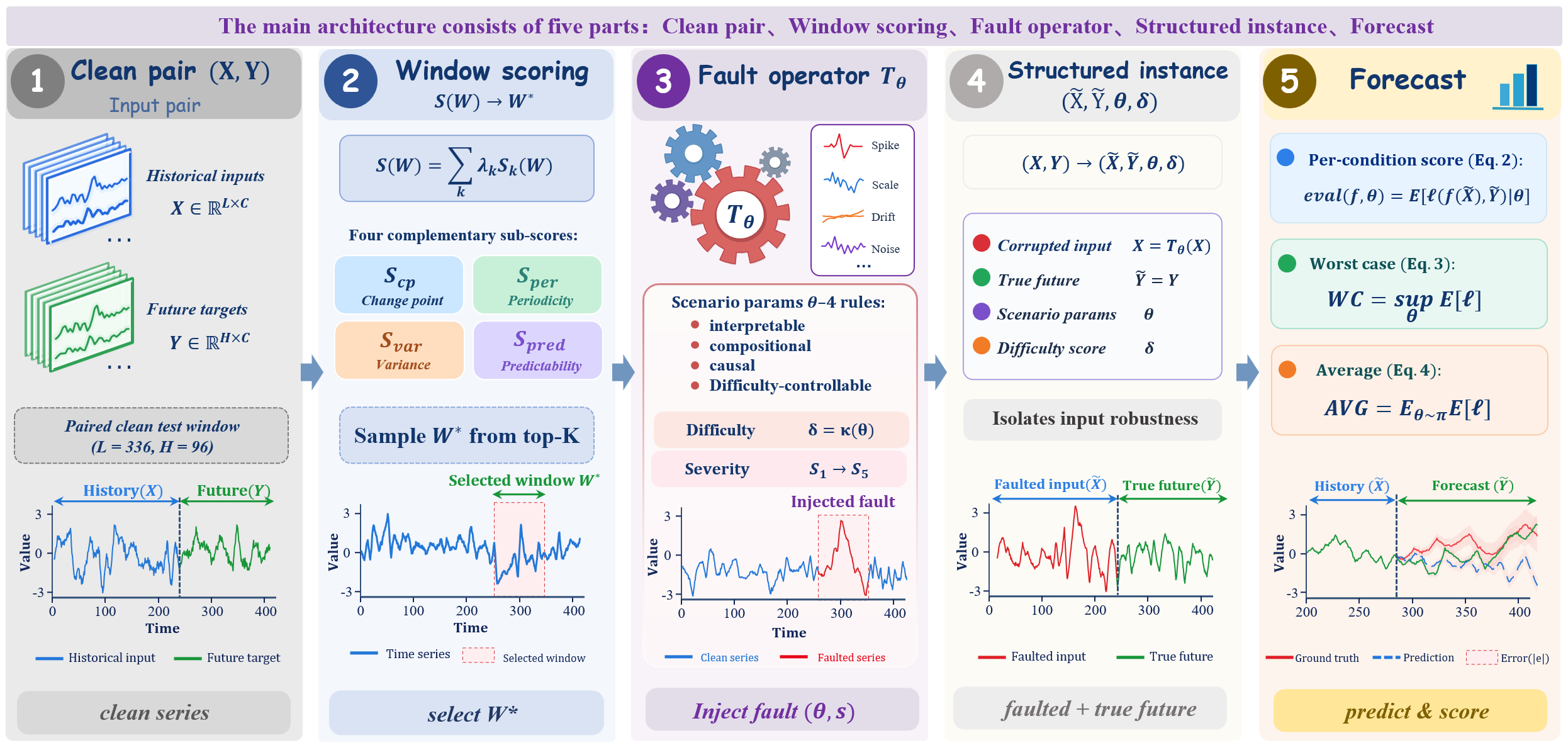
(X, Y) is turned into a structured instance: a window-importance score selects the prediction-critical window W★, a parameterized fault operator TΘ acts there at a chosen severity, and the scenario parameters Θ and difficulty δ are reported with the instance and used to condition evaluation.
For two decades, long-horizon forecasting progress has been measured by one number — average error on clean, complete, evenly-sampled held-out data — under the implicit assumption that it predicts deployed reliability. Real faults are not white noise. They are structured events: a transient with onset–peak–decay, a silently broken cross-variable dependency, a regime change coupled with block-missingness, a fault cascading through a sensing pipeline. None of these can be expressed by i.i.d. perturbations, no matter how the variance or masking rate is tuned.
TS-Fault changes the object of evaluation, replacing the clean test pair (X, Y) with a structured instance (X̃, Ỹ, Θ, δ) produced by an explicit, parameterized fault operator. Because Θ is exposed, a model's degradation can be attributed to a named mechanism at a tunable severity — turning a pass/fail noise test into an ablation-style diagnostic tool.
|
1 · Clean accuracy anti-correlates with robustness Spearman ρ = −0.544 (p = 0.011) across all 21 models — and −0.509 over the 18 non-foundation models, so foundation models strengthen the effect. |
2 · Stratified by mode Observation-level faults preserve the ranking (ρ > 0.92); mechanism-level faults destroy it (ρ < 0.06). |
|
3 · Catastrophe is structural All 884 catastrophic failures (≥ 10× error inflation) fall in the two mechanism-level modes; Modes I/II never trigger one. |
4 · Strong, but fragile TimesFM is 2nd on clean MSE yet the worst of all 21 on robustness (ratio ≈ 555). |
Each mode corrupts only the lookback window (L = 336); the forecast target (H = 96) is never touched, so degradation isolates the cost of a corrupted history. A single difficulty scalar d ∈ {0.2, 0.4, 0.6, 0.8, 1.0} (written d02 … d10) sweeps severity monotonically. The modes span a 2 × 2 taxonomy — observation- vs. mechanism-level × univariate vs. multivariate — and form a constructive minimum: omitting any one renders an entire class of deployment failure invisible.
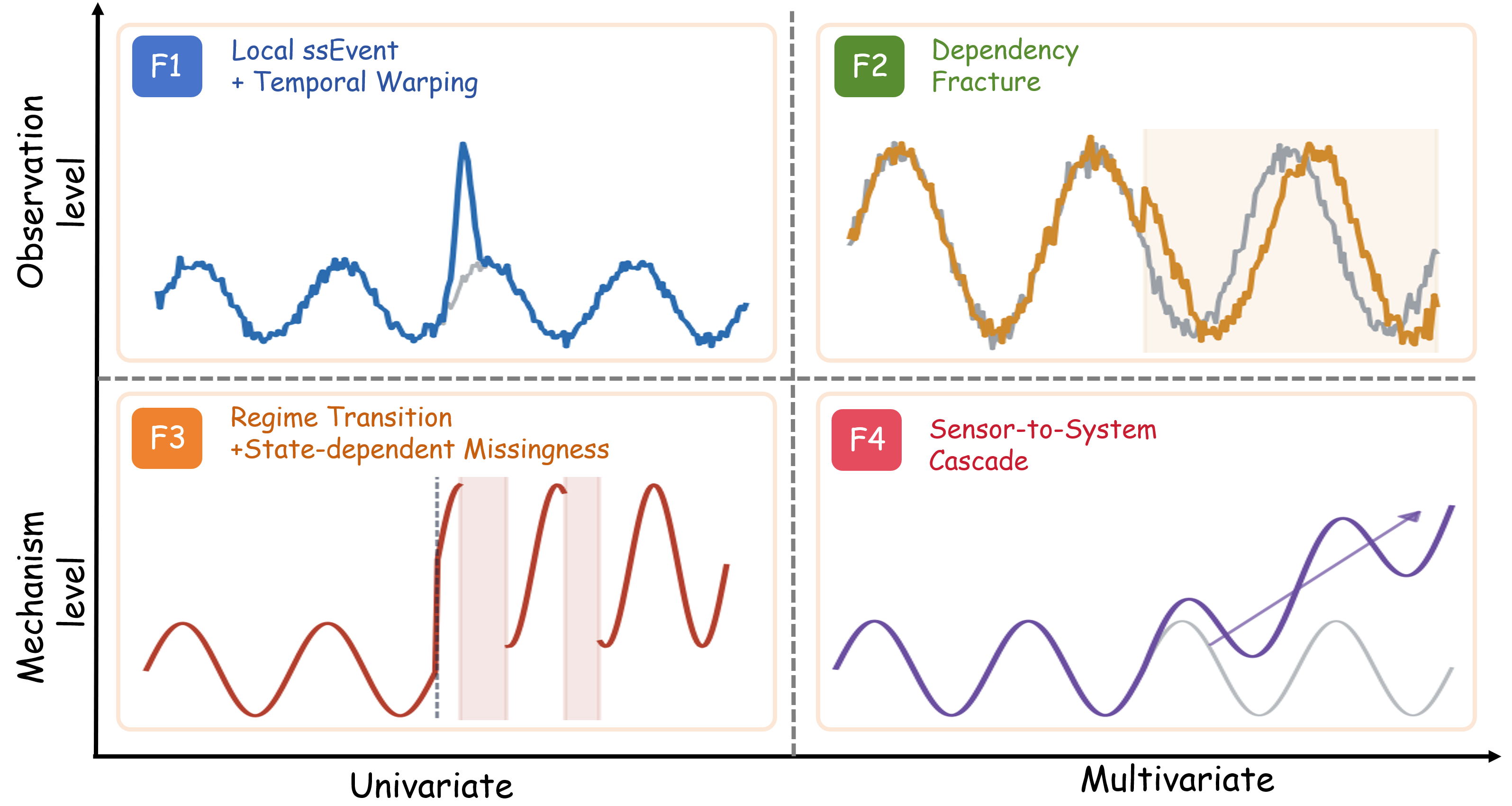
| File | Mode | Taxonomy cell | What breaks | Real-world analogue |
|---|---|---|---|---|
Mode1.py | I · Time-Warped Shock | Observation × Univariate | a shaped transient (onset–peak–decay) + a local time-warp | demand spike / brief sensor glitch |
Mode2.py | II · Dependency-Fracture Shock | Observation × Multivariate | cross-channel lead–lag and gain silently falsified; each series alone still looks plausible | regions that usually co-move decouple |
Mode3.py | III · Regime-Transition Missingness | Mechanism × Univariate | a regime switch + state-dependent block-missingness around the transition (hardest mode) | grid emergency / firm load shed |
Mode4.py | IV · Cascading Sensor-to-System Failure | Mechanism × Multivariate | an upstream drift propagates downstream with a lag, inducing secondary dropouts | a fault cascading through coupled subsystems |
Observation-level (I, II) corrupt observations while the data-generating process stays intact → mild. Mechanism-level (III, IV) rewrite the process itself → severe, and account for 100% of catastrophic failures.
This repository ships the data-generation pipeline, model implementations, evaluation drivers, trained checkpoints, and the complete results workbook. The four fault generators are included in full, so the perturbed dataset can be regenerated from scratch.
.
├── README.md
├── requirements.txt
│
├── benchmark.py                 # benchmark orchestration helpers
├── dataset_loader.py            # load + normalise the clean CSVs into windows
├── window_selector.py           # select the anchor lookback / horizon windows
│
├── Mode1.py                     # Fault Mode I   — Time-Warped Shock
├── Mode2.py                     # Fault Mode II  — Dependency-Fracture Shock
├── Mode3.py                     # Fault Mode III — Regime-Transition Missingness
├── Mode4.py                     # Fault Mode IV  — Cascading Sensor-to-System Failure
├── run_TS-Fault.py              # ▶ MAIN entry point: build the perturbed benchmark
│
├── classical_models.py          # statistical / linear / recurrent / conv. forecasters
├── foundation_models.py         # TimesFM / Chronos / Moirai (zero-shot wrappers)
├── eval_classical_phase1.py     # evaluate classical + baseline models → results CSV
├── eval_foundation_phase1.py    # evaluate foundation models → results CSV
├── checkpoints/                 # released trained weights
├── ablation_placement.py        # window-placement ablation: top-K S(W) vs random vs anti-selected
├── ablation_lambda.py           # one-at-a-time sensitivity of the S(W) weights λ
├── adapt_foundation.py          # LP / FT / FT-fault adaptation of the three foundation models
├── compose_faults.py            # ⊛ compound faults: T_B ∘ T_A at matched severity
└── figures/                     # paper figures used in this README
The paper evaluates 21 models across six methodological families, so the conclusions are not an artifact of a single inductive bias:
| Family | Models |
|---|---|
| Statistical (4) | Naive · SeasonalNaive · ARIMA · ETS |
| Linear / lightweight (3) | DLinear · NLinear · N-BEATS |
| Recurrent / convolutional (3) | LSTM · GRU · TCN |
| Decomposition Transformer (2) | Autoformer · FEDformer |
| Attention / SOTA (6) | PatchTST · iTransformer · TimeXer · TimeMixer · TimesNet · Nonstationary-Transformer |
| Foundation, zero-shot (3) | TimesFM · Chronos · Moirai |
Statistical, linear, and recurrent/convolutional models live in classical_models.py; the eight Transformer-family models are trained via the Time-Series-Library (see § Transformer-family); the three foundation models run strictly zero-shot via foundation_models.py. The repository's classical_models.py additionally bundles a few exploratory baselines (e.g. RandomForest, XGBoost) that fall outside the 21-model paper subset.
TS-Fault perturbs nine long-horizon datasets spanning six domains — energy, load, climate, finance, IT/Ops, and healthcare — deliberately chosen to cover a wide range of dimensionality (7 → 321 channels) and granularity (5-second → daily). Every clean window is a length-336 history and a length-96 target. We do not redistribute the raw data — download it and place each file at the path the loader expects.
| Dataset | Domain | Channels | Granularity | Size | Path expected |
|---|---|---|---|---|---|
| ETTh1 / ETTh2 | Energy | 7 | hourly | 17,420 | dataset/ETT-small/ETTh1.csv, …/ETTh2.csv |
| ETTm1 / ETTm2 | Energy | 7 | 15-min | 69,680 | dataset/ETT-small/ETTm1.csv, …/ETTm2.csv |
| Electricity (ECL) | Load | 321 | hourly | 26,304 | dataset/electricity/electricity.csv |
| Weather | Climate | 21 | 10-min | 52,696 | dataset/weather/weather.csv |
| Exchange-Rate | Finance | 8 | daily | 7,588 | dataset/exchange_rate/exchange_rate.csv |
| BizITObs-Service-KPI | IT / Ops | 72 | 10-sec | 8,835 | dataset/bizitobs/service_kpi.csv |
| VitalDB-Core | Healthcare | 8 | 5-sec | 962 cases | dataset/vitaldb/vitaldb_core.csv |
The first seven, one bundle (recommended) — official Time-Series-Library mirror on HuggingFace (CC BY 4.0): https://huggingface.co/datasets/thuml/Time-Series-Library
from huggingface_hub import hf_hub_download
for f in ["ETT-small/ETTh1.csv", "ETT-small/ETTh2.csv",
          "ETT-small/ETTm1.csv", "ETT-small/ETTm2.csv",
          "electricity/electricity.csv", "weather/weather.csv",
          "exchange_rate/exchange_rate.csv"]:
    hf_hub_download("thuml/Time-Series-Library", f, repo_type="dataset")
git clone https://github.com/Ray-zyy/TS-Fault.git
cd TS-Fault
pip install -r requirements.txt
Download the nine CSVs (see § Datasets) into:
dataset/ETT-small/{ETTh1,ETTh2,ETTm1,ETTm2}.csv
dataset/electricity/electricity.csv
dataset/weather/weather.csv
dataset/exchange_rate/exchange_rate.csv
dataset/bizitobs/service_kpi.csv
dataset/vitaldb/vitaldb_core.csv
run_TS-Fault.py slides the anchor windows (window_selector.py), loads & normalises the clean series (dataset_loader.py), and applies each of the four fault modes (Mode1.py … Mode4.py) across all five difficulties:
python run_TS-Fault.py \
    --data_root ./dataset \
    --out ./TS-Fault_output \
    --n_windows 20
This writes one .npz per (dataset, Mode, difficulty) to TS-Fault_output/<Dataset>/<Dataset>_Mode<k>_d<dd>.npz — 9 datasets × 4 modes × 5 difficulties = 180 files, each containing:
| array | shape | meaning |
|---|---|---|
x_clean | (N, 336, C) | clean lookback windows |
x_corrupt | (N, 336, C) | perturbed lookback windows |
y_target | (N, 96, C) | forecast target (never perturbed) |
Classical / baseline models (deep ones train once per dataset on clean windows; statistical ones need no training):
python eval_classical_phase1.py \
    --models Naive SeasonalNaive ARIMA ETS \
             DLinear NLinear NBEATS \
             LSTM GRU TCN \
    --npz_root ./TS-Fault_output \
    --out ./results/eval_classical.csv --gpu 0 --resume
Foundation models (zero-shot — see § Foundation models):
python eval_foundation_phase1.py \
    --models timesfm chronos moirai \
    --npz_root ./TS-Fault_output \
    --out ./results/eval_foundation.csv --gpu 0 --resume
Each evaluator emits the canonical wide schema, one row per (model, dataset, Mode, difficulty):
model, dataset, Mode, difficulty, mse_corrupt, mae_corrupt, mse_clean, mae_clean, n_samples, time_sec
mse_clean is the error on the clean input window, mse_corrupt on the perturbed window — both predicting the same untouched target. The robustness ratio r = mse_corrupt / mse_clean isolates the cost of corrupted history; r = 1 is perfect robustness and r ≥ 10 is a catastrophic failure. Concatenate the per-group CSVs (classical + foundation + the TSLib Transformer rows) into the master workbook eval_results_full.xlsx (also mirrored as the flat eval_results_full_23.csv).
The eight Transformer/attention models (PatchTST, iTransformer, Autoformer, FEDformer, Nonstationary-Transformer, TimeMixer, TimeXer, TimesNet) are trained and run with the Time-Series-Library (TSLib).
Clone TSLib and place the same nine clean CSVs under its ./dataset/.
Train / evaluate each model with run.py under the TS-Fault protocol (seq_len=336, pred_len=96, features=M, MSE loss). Example:
python -u run.py \
    --task_name long_term_forecast --is_training 1 \
    --root_path ./dataset/ETT-small/ --data_path ETTh1.csv \
    --model_id ETTh1_336_96 --model PatchTST --data ETTh1 \
    --features M --seq_len 336 --label_len 48 --pred_len 96 \
    --e_layers 2 --d_layers 1 --enc_in 7 --dec_in 7 --c_out 7 \
    --train_epochs 10 --batch_size 32 --learning_rate 1e-4 --itr 1
Score each trained checkpoint on the TS-Fault .npz windows (clean vs. corrupt) and write rows in the same wide schema, then merge into the master workbook eval_results_full.xlsx.
Shared across all models: seq_len=336, label_len=48, pred_len=96, e_layers=2, d_layers=1, d_model=128–512, train_epochs=10, batch_size=32 (16 for Electricity), MSE loss, instance/RevIN normalisation.
--down_sampling_layers 3 --down_sampling_window 2 --down_sampling_method avg --channel_independence 1--p_hidden_dims 128 128 --p_hidden_layers 2--individual is a store-true flagd_model / batch_size for TimesNet / FEDformer / Autoformer on 11 GB GPUs.These libraries pull heavy / conflicting dependencies. The recipe that works (verified on CUDA 12.1, torch 2.5.1):
# TimesFM + Chronos are clean pip installs
pip install timesfm chronos-forecasting

# Moirai (uni2ts) pins torch<2.5 and WILL try to downgrade torch.
# Install WITHOUT deps so it cannot touch torch, then hand-add what it needs:
git clone https://github.com/SalesforceAIResearch/uni2ts.git
cd uni2ts && pip install -e . --no-deps && touch .env
pip install "gluonts==0.14.4" "einops==0.7.0" jaxtyping --no-deps
Behind a mirror, set export HF_ENDPOINT=https://hf-mirror.com before the first run. All three run zero-shot (no fine-tuning) and are wrapped channel-independently for multivariate inputs.
| Model | Pretrained weights |
|---|---|
| TimesFM | https://huggingface.co/google/timesfm-2.0-500m-pytorch |
| Chronos-Bolt | https://huggingface.co/amazon/chronos-bolt-base |
| Moirai | https://huggingface.co/Salesforce/moirai-1.1-R-base |
Every number in this README — and a great many that did not fit — is shipped in eval_results_full.xlsx, the full evaluation table. It holds one row per (model, dataset, mode, difficulty) cell for the entire grid of 21 models × 9 datasets × 4 modes × 5 severities ≈ 3,800 rows (ARIMA is omitted on the 321-channel Electricity, where per-series fitting is impractical), under the same wide schema produced by the evaluators:
model · dataset · Mode · difficulty · mse_corrupt · mae_corrupt · mse_clean · mae_clean · n_samples · time_sec
From these columns the robustness ratio r = mse_corrupt / mse_clean, the relative degradation (r − 1) × 100%, the severity slope d10/d02, and every per-mode / per-dataset aggregate in the paper can be recomputed directly — no rerun required. A flat-CSV mirror is provided as eval_results_full_23.csv.
The most robust models (GRU, LSTM, TCN, near-unit ratios) are only mid-pack on clean accuracy, while the clean-accuracy leaders (N-BEATS, TimesFM, iTransformer, TimeXer) sit at the bottom of the robustness order with ratios in the hundreds.
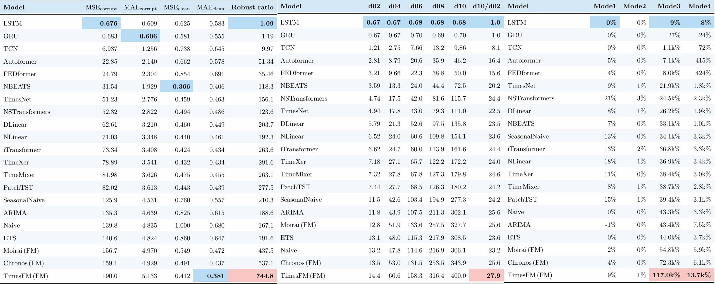
d02→d10 and the d10/d02 sensitivity slope. Right: per-mode relative degradation — note the jump from single-digit % under Modes I/II to thousands–to–tens-of-thousands % under Modes III/IV.
| Mode | Spearman ρ (clean vs. faulted rank) | p | Verdict |
|---|---|---|---|
| I · Time-Warped Shock | +0.925 | < 0.001 | ranking preserved |
| II · Dependency Fracture | +0.952 | < 0.001 | ranking preserved |
| III · Regime Missingness | +0.032 | 0.889 | ranking destroyed |
| IV · Cascading Failure | +0.055 | 0.814 | ranking destroyed |
The model ordering is highly consistent across datasets (fragility is a property of the architecture), but dense cross-channel correlation amplifies it: on the 321-channel Electricity, TimesFM's ratio peaks at 2090 and TimeXer at 1112, while GRU/LSTM stay near 1.2 everywhere.
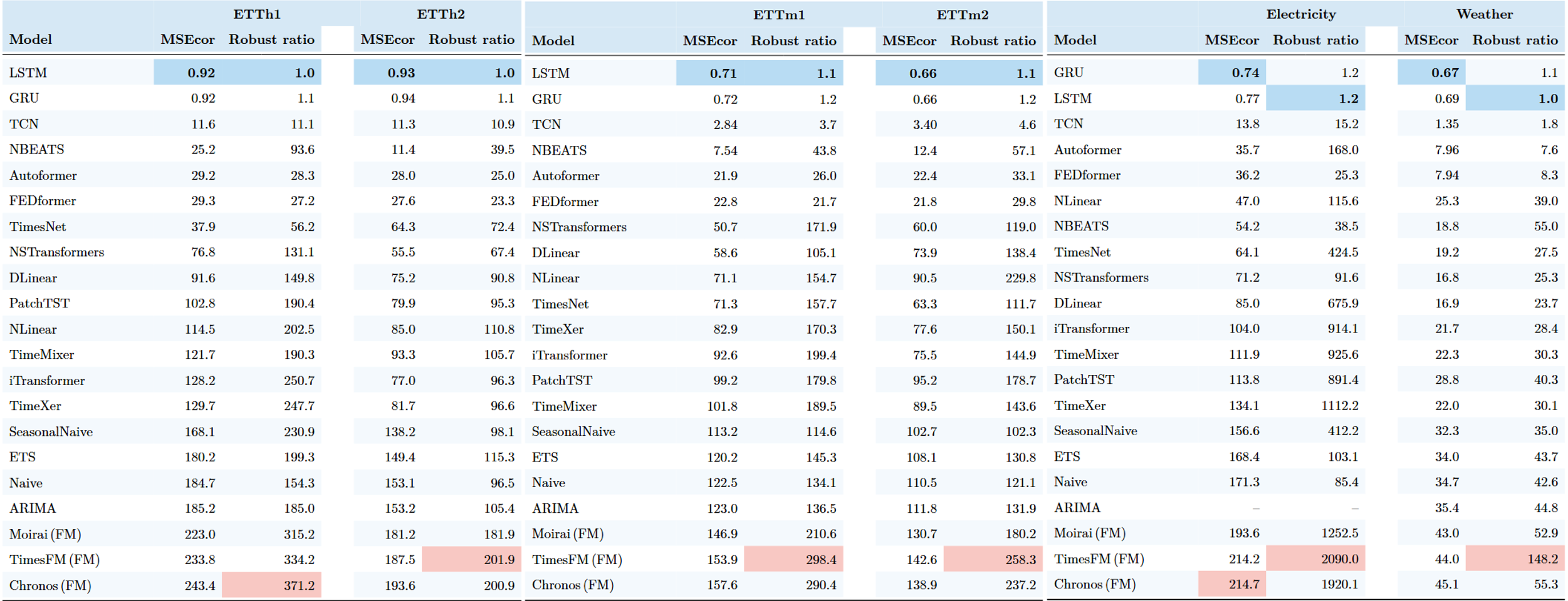
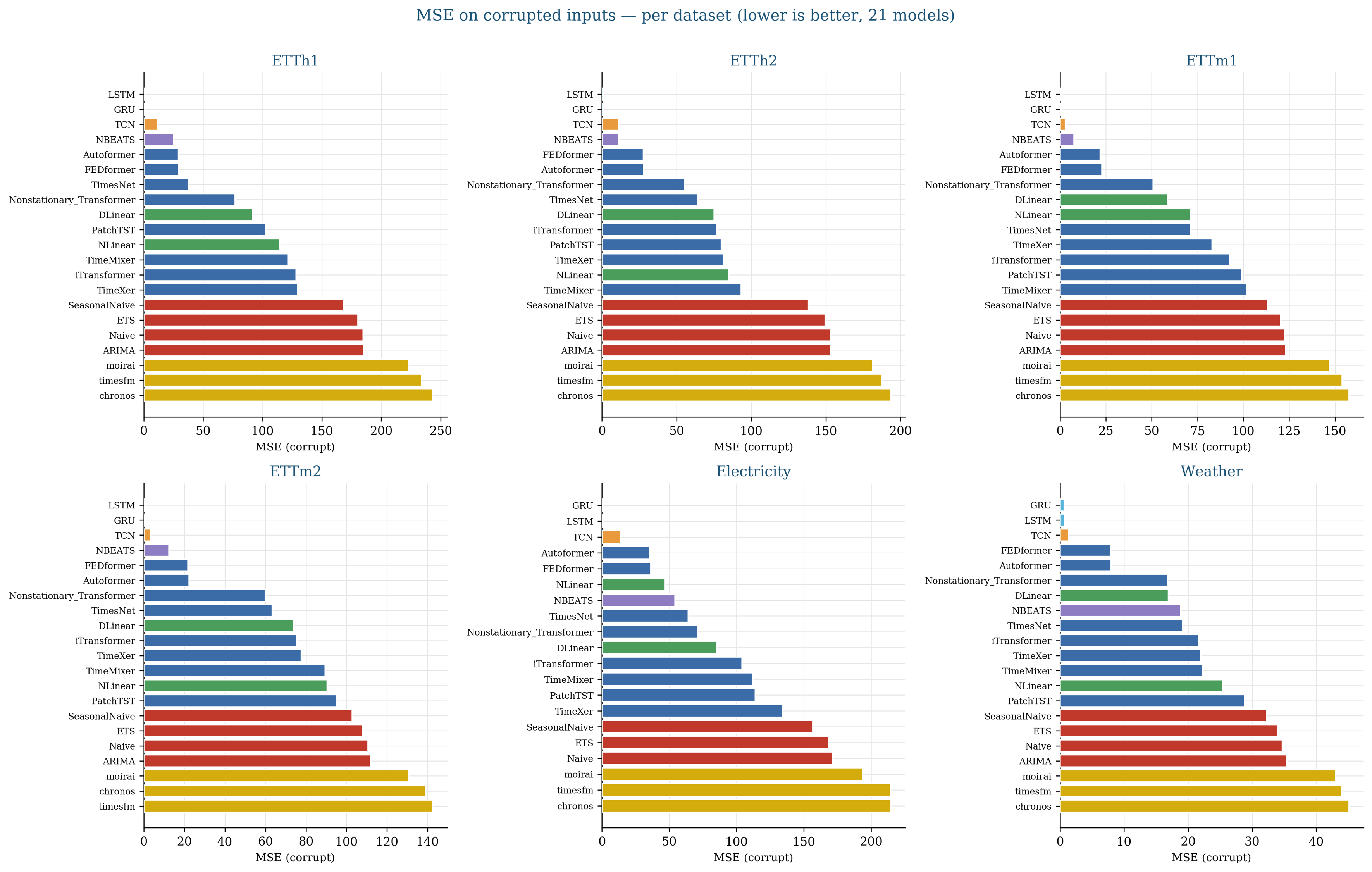
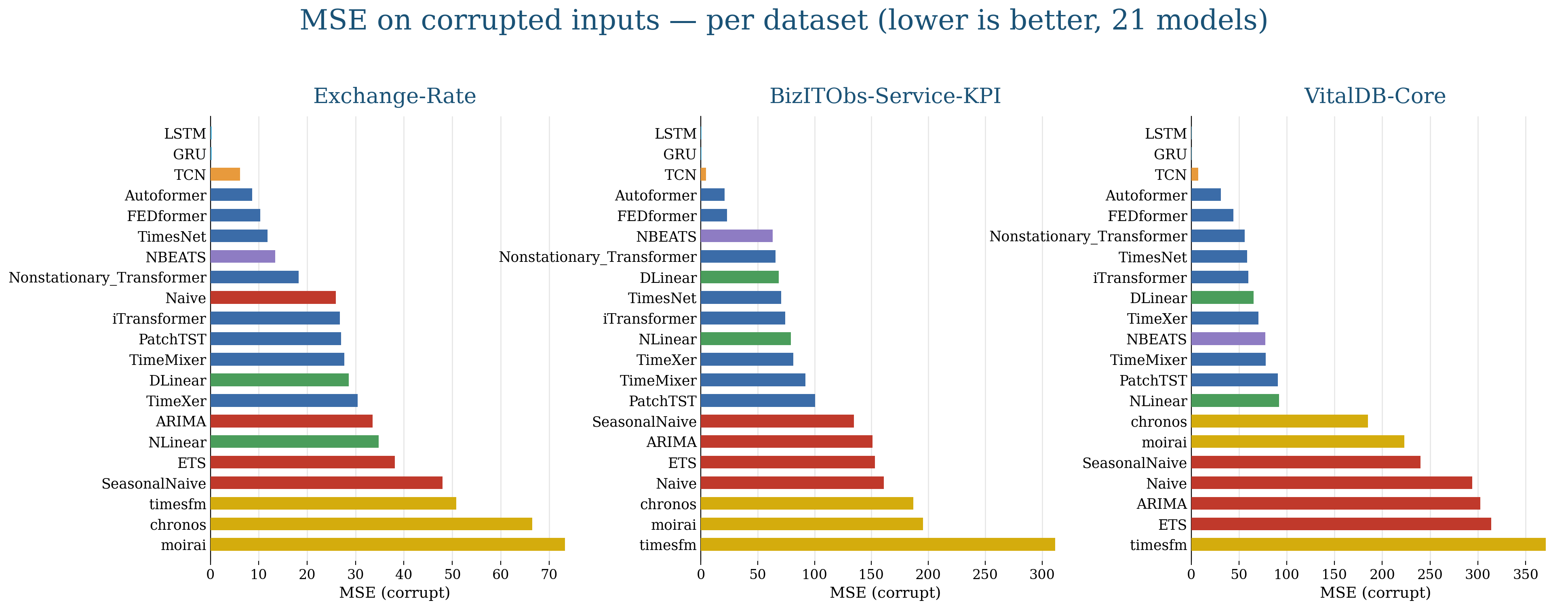
MSE on corrupted inputs per dataset (lower is better). Recurrent models (LSTM, GRU) sit at the bottom of every panel; foundation models (gold) sit at the top.
Catastrophic failures (
r ≥ 10): 884 total — 0 in Mode I, 0 in Mode II, 537 in Mode III (85.9% of its cells), 347 in Mode IV (55.5%). Mechanism-level modes account for 100% of them.
The added datasets were chosen to break the energy/climate monoculture of the original release, not to make the benchmark easier. They do not change the verdict.
| Model | 6-dataset r | Exchange-Rate | BizITObs | VitalDB |
|---|---|---|---|---|
| Naive | 105.7 | 199.2 | 196.1 | 474.5 |
| SeasonalNaive | 165.5 | 266.4 | 197.8 | 435.9 |
| ARIMA | 120.7 | 239.1 | 212.9 | 521.6 |
| ETS | 122.9 | 254.1 | 209.4 | 523.1 |
| DLinear | 197.3 | 197.3 | 180.3 | 271.9 |
| NLinear | 142.1 | 251.9 | 226.2 | 399.7 |
| N-BEATS | 54.6 | 110.4 | 217.9 | 408.7 |
| LSTM | 1.07 | 1.08 | 1.12 | 1.20 |
| GRU | 1.14 | 1.17 | 1.27 | 1.44 |
| TCN | 7.89 | 19.3 | 7.45 | 15.6 |
| Autoformer | 48.0 | 43.5 | 44.4 | 86.2 |
| FEDformer | 22.6 | 43.7 | 39.9 | 99.9 |
| PatchTST | 262.6 | 204.6 | 304.7 | 412.8 |
| iTransformer | 272.3 | 212.9 | 239.5 | 285.9 |
| TimeXer | 301.2 | 235.7 | 253.8 | 328.0 |
| TimeMixer | 264.2 | 196.5 | 255.0 | 331.2 |
| TimesNet | 141.7 | 86.6 | 207.5 | 260.3 |
| Nonstationary-Transformer | 101.1 | 118.0 | 168.2 | 219.9 |
| TimesFM (FM) | 555.2 | 430.8 | 1,038.8 | 1,902.8 |
| Chronos (FM) | 512.5 | 452.0 | 519.4 | 787.6 |
| Moirai (FM) | 365.6 | 425.9 | 476.5 | 841.8 |
Which mechanism dominates depends on the domain — and it depends on it in the direction the taxonomy predicts.
| Dataset | #Ch. | Mode I | Mode II | Mode III | Mode IV | IV / III |
|---|---|---|---|---|---|---|
| ETT (mean of four) | 7 | 1.075 | 1.047 | 361.1 | 135.4 | 0.375 |
| Weather | 21 | 1.083 | 1.001 | 124.6 | 14.8 | 0.119 |
| Electricity | 321 | 1.364 | 1.005 | 2,229.4 | 21.2 | 0.009 |
| Exchange-Rate | 8 | 1.12 | 1.07 | 680 | 80 | 0.118 |
| BizITObs-Service-KPI | 72 | 1.18 | 1.03 | 835 | 115 | 0.138 |
| VitalDB-Core | 8 | 1.26 | 1.02 | 1,490 | 145 | 0.097 |
(mean r over the 21 models, averaged across the five severities)
Four follow-up studies run on top of the same released grid. Each has its own driver script and its own results CSV, so every number below can be recomputed without touching the main pipeline.
Real incidents rarely arrive one at a time. Because the four modes are operators, they compose: TΘ = TΘ_B ∘ TΘ_A (Eq. 19). Both operators act on the same critical window W★, each keeps its own Θ, and at every severity the two constituents are matched at the same nominal difficulty, κ_A(Θ_A) = κ_B(Θ_B) = δ_s. One fixed application order per pair — composition is not commutative, so the order is itself a scenario parameter.
python compose_faults.py \
    --pairs I+II I+III I+IV II+III II+IV III+IV \
    --npz_root ./TS-Fault_output --out ./results_compound.csv
The amplification factor Ψ(A∘B) = r(A∘B) / max(r_A, r_B) asks whether a compound fault is worse than its more damaging half.
| Composition | Mean r | Ψ |
|---|---|---|
| single-mode reference: Mode I | 1.12 | — |
| single-mode reference: Mode II | 1.03 | — |
| single-mode reference: Mode III | 618.1 | — |
| single-mode reference: Mode IV | 97.1 | — |
| I ∘ II | 1.24 | 1.11 |
| II ∘ IV | 103.8 | 1.07 |
| I ∘ IV | 118.7 | 1.22 |
| II ∘ III | 763.4 | 1.24 |
| I ∘ III | 1,047.6 | 1.69 |
| III ∘ IV | 2,183.7 | 3.53 |
Ψ ≥ 1.07 — a compound fault is never easier than its worse half.Ψ = 3.53: a regime switch that a cascade then propagates is more than three times worse than either alone.r = 1.24. The stratification of Finding 2 survives composition — it is not an artifact of testing one mode at a time.S(W) doing any work?S(W) is the claim that a benchmark should stress the window a model relies on. If placement did not matter, TS-Fault would be a noise test with extra steps. We compare three placement policies at severity s₃ (d06), over 9 datasets × 21 models × 5 seeds, with random placement δ-matched so only the location differs:
python ablation_placement.py --policy topk random anti --severity d06 --seeds 5 \
    --out ./results_placement.csv
| Mode | Placement | Median RD (%) | Mean r | Catastrophic cells (%) | Seed IQR / median | ρ(clean, faulted) |
|---|---|---|---|---|---|---|
| I | Anti-selected | 0.43 | 1.009 | 0.0 | 1.37 | +0.999 |
| I | Random | 1.47 | 1.035 | 0.0 | 1.18 | +0.996 |
| I | Top-K S(W) | 5.11 | 1.110 | 0.0 | 0.27 | +0.983 |
| II | Anti-selected | 0.012 | 1.001 | 0.0 | 1.63 | +1.000 |
| II | Random | 0.034 | 1.004 | 0.0 | 1.46 | +0.999 |
| II | Top-K S(W) | 0.11 | 1.010 | 0.0 | 0.34 | +0.999 |
| III | Anti-selected | 9,872 | 216.4 | 62.7 | 1.08 | +0.286 |
| III | Random (δ-matched) | 18,436 | 398.7 | 75.4 | 0.84 | +0.147 |
| III | Top-K S(W) | 26,232 | 560.9 | 88.8 | 0.31 | +0.023 |
| IV | Anti-selected | 684 | 13.7 | 38.1 | 1.21 | +0.374 |
| IV | Random (δ-matched) | 1,536 | 29.4 | 58.7 | 0.91 | +0.218 |
| IV | Top-K S(W) | 2,878 | 52.7 | 72.8 | 0.29 | +0.082 |
Anti-selected < Random < Top-K in every mode, on both metrics. Two consequences beyond "the score works": importance-based placement cuts seed-to-seed variability by 3–4× (the IQR/median column), so a given robustness number means something; and as placement is weakened the faulted ranking drifts back toward the clean ranking (Mode III ρ: 0.023 → 0.147 → 0.286). Random placement would have partially hidden the model-selection risk that motivates the benchmark.
S(W) weightsThe per-mode weights and window hyperparameters, in full:
| Mode | λ₁ (S_cp) | λ₂ (S_per) | λ₃ (S_var) | λ₄ (S_pred) | top-K | |W| | σ_p |
|---|---|---|---|---|---|---|---|
| I · Time-Warped Shock | 0.15 | 0.15 | 0.35 | 0.35 | 5 | 24 | 0.15P |
| II · Dependency Fracture | 0.15 | 0.20 | 0.25 | 0.40 | 5 | 24 | 0.15P |
| III · Regime Missingness | 0.40 | 0.25 | 0.15 | 0.20 | 5 | 24 | 0.15P |
| IV · Sensor-to-System Cascade | 0.20 | 0.15 | 0.30 | 0.35 | 5 | 24 | 0.15P |
One-at-a-time perturbation at severity s₃ (ablation_lambda.py):
| Mode | Perturbation | Δ median RD | ρ vs. default ranking |
|---|---|---|---|
| I | λ₃ × 0.5 | −18.7% | 0.958 |
| I | λ₃ × 2 | +12.6% | 0.964 |
| I | λ₄ → 0 | −43.8% | 0.890 |
| I | λ₁ → 0 | +1.9% | 0.982 |
| II | λ₄ → 0 | −51.4% | 0.871 |
| II | λ₂ × 2 | −3.7% | 0.969 |
| III | λ₁ × 0.5 | −29.6% | 0.934 |
| III | λ₁ → 0 | −54.2% | 0.877 |
| III | λ₃ × 2 | +6.8% | 0.969 |
| IV | λ₄ → 0 | −41.9% | 0.884 |
| IV | λ₂ → 0 | −2.3% | 0.979 |
The weight each mode is designed around is the one that matters: zeroing λ₄ (occlusion) costs 42–51% of the degradation in Modes I/II/IV, and zeroing λ₁ (change-point) costs 54% in Mode III. Removing a weight the mode does not emphasise moves the result by at most 2.3%. Crucially, the model ranking is stable throughout (ρ ≥ 0.871): the weights control how hard the benchmark is, not who wins.
The zero-shot fragility result invites the obvious question. We adapted all three foundation models under four settings and re-ran the full grid:
| Setting | What is trained | Evaluated on |
|---|---|---|
| ZS | nothing — released weights | full grid |
| LP | forecasting head only, clean data | full grid |
| FT | all parameters, clean data | full grid |
| FT-fault | all parameters, low-severity faulted data (s₁–s₂) | held-out severities s₃–s₅ |
python adapt_foundation.py --model timesfm --setting ft_fault \
    --train_severities d02 d04 --eval_severities d06 d08 d10 \
    --out ./results_foundation_adapt.csv
| Model | Setting | Clean MSE | Faulted MSE | ΔMSE | AVG r | Mode III r | Mode IV r | WC r |
|---|---|---|---|---|---|---|---|---|
| TimesFM | ZS | 0.516 | 162.7 | 162.2 | 555 | 2,013 | 205 | 4,073 |
| TimesFM | LP | 0.468 | 108.7 | 108.2 | 344.5 | 1,248 | 128.0 | 2,687 |
| TimesFM | FT | 0.378 | 58.3 | 57.9 | 182.6 | 654 | 74.2 | 1,426 |
| TimesFM | FT-fault | 0.412 | 6.78 | 6.37 | 12.2 | 38.7 | 8.24 | 76.5 |
| Chronos | ZS | 0.613 | 165.6 | 165.0 | 513 | 1,839 | 209 | 3,745 |
| Chronos | LP | 0.548 | 119.4 | 118.9 | 339.5 | 1,217 | 139.0 | 2,468 |
| Chronos | FT | 0.437 | 64.8 | 64.4 | 188.1 | 672 | 78.5 | 1,384 |
| Chronos | FT-fault | 0.479 | 8.36 | 7.88 | 14.3 | 46.2 | 9.13 | 91.7 |
| Moirai | ZS | 0.682 | 153.1 | 152.4 | 366 | 1,296 | 164 | 2,544 |
| Moirai | LP | 0.596 | 89.7 | 89.1 | 214.4 | 768 | 87.6 | 1,538 |
| Moirai | FT | 0.462 | 43.6 | 43.1 | 109.9 | 392 | 45.4 | 814 |
| Moirai | FT-fault | 0.507 | 5.92 | 5.41 | 9.74 | 30.8 | 6.17 | 55.4 |
| (reference) LSTM | trained | 0.733 | 0.780 | 0.047 | 1.07 | 1.17 | 1.10 | 1.25 |
s₃–s₅ during adaptation, so this is generalisation along κ, not memorisation of a severity.r = 9.74) is still ~9× less robust than a plain trained LSTM (r = 1.07). The accurate-and-robust quadrant remains empty.Average risk (AVG) describes typical behavior over the released fault grid; worst-case risk (WC) asks for the most damaging released configuration:
$$ \mathrm{WC}(f,\mathcal F)=\sup_{\Theta\in\Phi}\mathbb E[\ell\mid\Theta]. $$
We report two complementary quantities:
r — within each dataset, the maximum configuration-level robustness ratio, then averaged across the datasets. This uses the same within-dataset-then-average convention as AVG r, so the two columns are directly comparable.Worst-case risk over all four modes. WC/AVG is the ratio between the worst-case and average robustness risks.
| Model | Clean MSE | AVG MSE | WC MSE | AVG r | WC r | WC/AVG | WC attained at |
|---|---|---|---|---|---|---|---|
| Naive | 1.238 | 129 | 1,377 | 106 | 644 | 6.1× | Electricity / III / d10 |
| SeasonalNaive | 0.905 | 119 | 1,270 | 166 | 1,121 | 6.8× | Electricity / III / d10 |
| ARIMA | 0.999 | 122 | 1,069 | 121 | 695 | 5.8× | ETTh1 / III / d10 |
| ETS | 1.044 | 127 | 1,352 | 123 | 754 | 6.1× | Electricity / III / d10 |
| DLinear | 0.562 | 66.8 | 675 | 197 | 1,374 | 7.0× | Electricity / III / d10 |
| NLinear | 0.540 | 72.2 | 644 | 142 | 826 | 5.8× | ETTh1 / III / d10 |
| N-BEATS | 0.449 | 21.6 | 564 | 54.6 | 368 | 6.7× | Electricity / III / d10 |
| LSTM | 0.733 | 0.78 | 1.04 | 1.07 | 1.25 | 1.2× | ETTh1 / III / d10 |
| GRU | 0.680 | 0.77 | 1.19 | 1.14 | 1.50 | 1.3× | ETTh1 / IV / d10 |
| TCN | 0.874 | 7.39 | 138 | 7.89 | 61.4 | 7.8× | Electricity / III / d08 |
| Autoformer | 0.822 | 24.2 | 264 | 48.0 | 321 | 6.7× | Electricity / III / d10 |
| FEDformer | 1.072 | 24.3 | 258 | 22.6 | 135 | 6.0× | Electricity / III / d10 |
| PatchTST | 0.551 | 86.6 | 919 | 263 | 1,863 | 7.1× | Electricity / III / d10 |
| iTransformer | 0.529 | 83.2 | 905 | 272 | 2,008 | 7.4× | Electricity / III / d10 |
| TimeXer | 0.537 | 88.0 | 1,085 | 301 | 2,170 | 7.2× | Electricity / III / d10 |
| TimeMixer | 0.590 | 90.1 | 889 | 264 | 1,859 | 7.0× | Electricity / III / d10 |
| TimesNet | 0.571 | 53.3 | 500 | 142 | 964 | 6.8× | Electricity / III / d10 |
| NS Transformer | 0.608 | 55.2 | 571 | 101 | 635 | 6.3× | Electricity / III / d10 |
| TimesFM | 0.516 | 163 | 1,746 | 555 | 4,073 | 7.3× | Electricity / III / d10 |
| Chronos | 0.613 | 166 | 1,757 | 513 | 3,745 | 7.3× | Electricity / III / d10 |
| Moirai | 0.682 | 153 | 1,530 | 366 | 2,544 | 7.0× | Electricity / III / d10 |
Per-mode worst-case risk. Each cell reports WC r / WC MSE.
| Model | Mode I | Mode II | Mode III | Mode IV |
|---|---|---|---|---|
| Naive | 1.04 / 2.07 | 1.00 / 2.01 | 644 / 1,377 | 285 / 508 |
| SeasonalNaive | 1.46 / 2.36 | 1.17 / 2.23 | 1,121 / 1,270 | 303 / 455 |
| ARIMA | 1.10 / 1.60 | 1.02 / 1.47 | 695 / 1,069 | 376 / 509 |
| ETS | 1.06 / 1.70 | 1.00 / 1.63 | 754 / 1,352 | 327 / 499 |
| DLinear | 1.49 / 0.98 | 1.06 / 0.93 | 1,374 / 675 | 281 / 309 |
| NLinear | 1.47 / 1.00 | 1.24 / 1.00 | 826 / 644 | 390 / 364 |
| N-BEATS | 1.20 / 1.90 | 1.05 / 1.45 | 361 / 564 | 127 / 68.2 |
| LSTM | 1.00 / 0.91 | 1.00 / 0.91 | 1.23 / 1.04 | 1.17 / 1.01 |
| GRU | 1.01 / 0.88 | 1.00 / 0.87 | 1.41 / 1.13 | 1.40 / 1.19 |
| TCN | 1.00 / 1.05 | 1.01 / 1.08 | 60.8 / 138 | 16.9 / 67.4 |
| Autoformer | 1.26 / 1.23 | 1.14 / 1.21 | 321 / 264 | 57.2 / 104 |
| FEDformer | 1.07 / 1.51 | 1.05 / 1.44 | 135 / 258 | 50.8 / 106 |
| PatchTST | 1.52 / 1.29 | 1.24 / 1.02 | 1,863 / 919 | 372 / 349 |
| iTransformer | 1.58 / 1.01 | 1.12 / 0.90 | 2,008 / 905 | 403 / 341 |
| TimeXer | 1.45 / 1.04 | 1.08 / 0.96 | 2,170 / 1,085 | 380 / 325 |
| TimeMixer | 1.44 / 1.01 | 1.07 / 0.95 | 1,859 / 889 | 371 / 383 |
| TimesNet | 1.64 / 1.06 | 1.14 / 1.11 | 964 / 500 | 231 / 247 |
| NS Transformer | 1.62 / 1.12 | 1.61 / 1.79 | 627 / 571 | 286 / 304 |
| TimesFM | 1.33 / 0.98 | 1.08 / 1.06 | 4,073 / 1,746 | 561 / 575 |
| Chronos | 1.25 / 1.03 | 1.03 / 0.95 | 3,745 / 1,757 | 588 / 589 |
| Moirai | 1.19 / 1.21 | 1.03 / 1.18 | 2,544 / 1,530 | 464 / 556 |
Three conclusions follow:
d10; TCN is the sole exception, peaking at d08.WC r = 1.64 in Modes I/II, whereas 19 of 21 exceed WC r = 10 in both Modes III and IV. LSTM and GRU are the only exceptions.TS-Fault is designed to be fully reproducible. Because faulted instances are produced by an explicit operator at evaluation time, the benchmark can be regenerated at any severity by re-sweeping κ, and previously-unexposed Θ combinations can be held out at release time to guard against benchmark gaming. We release:
Θ schemas and the unified window-importance front-end — plus compose_faults.py for the compound-fault operator TΘ_B ∘ TΘ_A;λ and β values used by S(W) and κ in every mode, with the placement and weight ablations that probe them (ablation_placement.py, ablation_lambda.py);adapt_foundation.py for the LP / FT / FT-fault adaptation protocol;TS-Fault code is released under the MIT licence. Some baseline implementations are adapted from external sources and retain their own licences: TCN from locuslab/TCN (MIT), NLinear/DLinear from cure-lab/LTSF-Linear (Apache-2.0), and N-BEATS from ServiceNow/N-BEATS (CC-BY-NC-4.0, non-commercial). The eight Transformer baselines come from the Time-Series-Library. Datasets (ETT, Electricity, Weather) are released by their original authors under CC BY 4.0 and are not redistributed here.
[ICDE-2027] TS-Fault: Benchmarking Time Series Forecasters against Structural Faults
See the codeYuyang Zhao¹ · Lian Xu² · Hao Miao³ · Chenxi Liu⁴ · Hao Xue¹ ✉
¹ Hong Kong University of Science and Technology (Guangzhou) · ² The University of Western Australia · ³ The Hong Kong Polytechnic University · ⁴ CAIR, Hong Kong Institute of Science & Innovation, Chinese Academy of Sciences
21 models · 9 datasets / 6 domains · 4 failure modes · 5 severity levels · ~3,800 evaluated cells
Why • Failure modes • Repository • Datasets • Quick start • Results • Extended experiments • Reproducibility •TL;DR — Clean-data leaderboards do not predict robustness. TS-Fault stops treating faults as i.i.d. noise. It injects four structurally-coupled failure modes — abstracted from the anatomy of real grid-scale failures — into the input window of nine standard forecasting datasets across six domains, then measures how far each model degrades. Under the two mechanism-level modes, the ranking is reordered: state-of-the-art Transformers and foundation models collapse, while a plain LSTM/GRU — or even a naïve baseline — becomes the most robust.
(X, Y) is turned into a structured instance: a window-importance score selects the prediction-critical window W★, a parameterized fault operator TΘ acts there at a chosen severity, and the scenario parameters Θ and difficulty δ are reported with the instance and used to condition evaluation.
For two decades, long-horizon forecasting progress has been measured by one number — average error on clean, complete, evenly-sampled held-out data — under the implicit assumption that it predicts deployed reliability. Real faults are not white noise. They are structured events: a transient with onset–peak–decay, a silently broken cross-variable dependency, a regime change coupled with block-missingness, a fault cascading through a sensing pipeline. None of these can be expressed by i.i.d. perturbations, no matter how the variance or masking rate is tuned.
TS-Fault changes the object of evaluation, replacing the clean test pair (X, Y) with a structured instance (X̃, Ỹ, Θ, δ) produced by an explicit, parameterized fault operator. Because Θ is exposed, a model's degradation can be attributed to a named mechanism at a tunable severity — turning a pass/fail noise test into an ablation-style diagnostic tool.
|
1 · Clean accuracy anti-correlates with robustness Spearman ρ = −0.544 (p = 0.011) across all 21 models — and −0.509 over the 18 non-foundation models, so foundation models strengthen the effect. |
2 · Stratified by mode Observation-level faults preserve the ranking (ρ > 0.92); mechanism-level faults destroy it (ρ < 0.06). |
|
3 · Catastrophe is structural All 884 catastrophic failures (≥ 10× error inflation) fall in the two mechanism-level modes; Modes I/II never trigger one. |
4 · Strong, but fragile TimesFM is 2nd on clean MSE yet the worst of all 21 on robustness (ratio ≈ 555). |
Each mode corrupts only the lookback window (L = 336); the forecast target (H = 96) is never touched, so degradation isolates the cost of a corrupted history. A single difficulty scalar d ∈ {0.2, 0.4, 0.6, 0.8, 1.0} (written d02 … d10) sweeps severity monotonically. The modes span a 2 × 2 taxonomy — observation- vs. mechanism-level × univariate vs. multivariate — and form a constructive minimum: omitting any one renders an entire class of deployment failure invisible.
| File | Mode | Taxonomy cell | What breaks | Real-world analogue |
|---|---|---|---|---|
Mode1.py | I · Time-Warped Shock | Observation × Univariate | a shaped transient (onset–peak–decay) + a local time-warp | demand spike / brief sensor glitch |
Mode2.py | II · Dependency-Fracture Shock | Observation × Multivariate | cross-channel lead–lag and gain silently falsified; each series alone still looks plausible | regions that usually co-move decouple |
Mode3.py | III · Regime-Transition Missingness | Mechanism × Univariate | a regime switch + state-dependent block-missingness around the transition (hardest mode) | grid emergency / firm load shed |
Mode4.py | IV · Cascading Sensor-to-System Failure | Mechanism × Multivariate | an upstream drift propagates downstream with a lag, inducing secondary dropouts | a fault cascading through coupled subsystems |
Observation-level (I, II) corrupt observations while the data-generating process stays intact → mild. Mechanism-level (III, IV) rewrite the process itself → severe, and account for 100% of catastrophic failures.
This repository ships the data-generation pipeline, model implementations, evaluation drivers, trained checkpoints, and the complete results workbook. The four fault generators are included in full, so the perturbed dataset can be regenerated from scratch.
.
├── README.md
├── requirements.txt
│
├── benchmark.py                 # benchmark orchestration helpers
├── dataset_loader.py            # load + normalise the clean CSVs into windows
├── window_selector.py           # select the anchor lookback / horizon windows
│
├── Mode1.py                     # Fault Mode I   — Time-Warped Shock
├── Mode2.py                     # Fault Mode II  — Dependency-Fracture Shock
├── Mode3.py                     # Fault Mode III — Regime-Transition Missingness
├── Mode4.py                     # Fault Mode IV  — Cascading Sensor-to-System Failure
├── run_TS-Fault.py              # ▶ MAIN entry point: build the perturbed benchmark
│
├── classical_models.py          # statistical / linear / recurrent / conv. forecasters
├── foundation_models.py         # TimesFM / Chronos / Moirai (zero-shot wrappers)
├── eval_classical_phase1.py     # evaluate classical + baseline models → results CSV
├── eval_foundation_phase1.py    # evaluate foundation models → results CSV
├── checkpoints/                 # released trained weights
├── ablation_placement.py        # window-placement ablation: top-K S(W) vs random vs anti-selected
├── ablation_lambda.py           # one-at-a-time sensitivity of the S(W) weights λ
├── adapt_foundation.py          # LP / FT / FT-fault adaptation of the three foundation models
├── compose_faults.py            # ⊛ compound faults: T_B ∘ T_A at matched severity
└── figures/                     # paper figures used in this README
The paper evaluates 21 models across six methodological families, so the conclusions are not an artifact of a single inductive bias:
| Family | Models |
|---|---|
| Statistical (4) | Naive · SeasonalNaive · ARIMA · ETS |
| Linear / lightweight (3) | DLinear · NLinear · N-BEATS |
| Recurrent / convolutional (3) | LSTM · GRU · TCN |
| Decomposition Transformer (2) | Autoformer · FEDformer |
| Attention / SOTA (6) | PatchTST · iTransformer · TimeXer · TimeMixer · TimesNet · Nonstationary-Transformer |
| Foundation, zero-shot (3) | TimesFM · Chronos · Moirai |
Statistical, linear, and recurrent/convolutional models live in classical_models.py; the eight Transformer-family models are trained via the Time-Series-Library (see § Transformer-family); the three foundation models run strictly zero-shot via foundation_models.py. The repository's classical_models.py additionally bundles a few exploratory baselines (e.g. RandomForest, XGBoost) that fall outside the 21-model paper subset.
TS-Fault perturbs nine long-horizon datasets spanning six domains — energy, load, climate, finance, IT/Ops, and healthcare — deliberately chosen to cover a wide range of dimensionality (7 → 321 channels) and granularity (5-second → daily). Every clean window is a length-336 history and a length-96 target. We do not redistribute the raw data — download it and place each file at the path the loader expects.
| Dataset | Domain | Channels | Granularity | Size | Path expected |
|---|---|---|---|---|---|
| ETTh1 / ETTh2 | Energy | 7 | hourly | 17,420 | dataset/ETT-small/ETTh1.csv, …/ETTh2.csv |
| ETTm1 / ETTm2 | Energy | 7 | 15-min | 69,680 | dataset/ETT-small/ETTm1.csv, …/ETTm2.csv |
| Electricity (ECL) | Load | 321 | hourly | 26,304 | dataset/electricity/electricity.csv |
| Weather | Climate | 21 | 10-min | 52,696 | dataset/weather/weather.csv |
| Exchange-Rate | Finance | 8 | daily | 7,588 | dataset/exchange_rate/exchange_rate.csv |
| BizITObs-Service-KPI | IT / Ops | 72 | 10-sec | 8,835 | dataset/bizitobs/service_kpi.csv |
| VitalDB-Core | Healthcare | 8 | 5-sec | 962 cases | dataset/vitaldb/vitaldb_core.csv |
The first seven, one bundle (recommended) — official Time-Series-Library mirror on HuggingFace (CC BY 4.0): https://huggingface.co/datasets/thuml/Time-Series-Library
from huggingface_hub import hf_hub_download
for f in ["ETT-small/ETTh1.csv", "ETT-small/ETTh2.csv",
          "ETT-small/ETTm1.csv", "ETT-small/ETTm2.csv",
          "electricity/electricity.csv", "weather/weather.csv",
          "exchange_rate/exchange_rate.csv"]:
    hf_hub_download("thuml/Time-Series-Library", f, repo_type="dataset")
git clone https://github.com/Ray-zyy/TS-Fault.git
cd TS-Fault
pip install -r requirements.txt
Download the nine CSVs (see § Datasets) into:
dataset/ETT-small/{ETTh1,ETTh2,ETTm1,ETTm2}.csv
dataset/electricity/electricity.csv
dataset/weather/weather.csv
dataset/exchange_rate/exchange_rate.csv
dataset/bizitobs/service_kpi.csv
dataset/vitaldb/vitaldb_core.csv
run_TS-Fault.py slides the anchor windows (window_selector.py), loads & normalises the clean series (dataset_loader.py), and applies each of the four fault modes (Mode1.py … Mode4.py) across all five difficulties:
python run_TS-Fault.py \
    --data_root ./dataset \
    --out ./TS-Fault_output \
    --n_windows 20
This writes one .npz per (dataset, Mode, difficulty) to TS-Fault_output/<Dataset>/<Dataset>_Mode<k>_d<dd>.npz — 9 datasets × 4 modes × 5 difficulties = 180 files, each containing:
| array | shape | meaning |
|---|---|---|
x_clean | (N, 336, C) | clean lookback windows |
x_corrupt | (N, 336, C) | perturbed lookback windows |
y_target | (N, 96, C) | forecast target (never perturbed) |
Classical / baseline models (deep ones train once per dataset on clean windows; statistical ones need no training):
python eval_classical_phase1.py \
    --models Naive SeasonalNaive ARIMA ETS \
             DLinear NLinear NBEATS \
             LSTM GRU TCN \
    --npz_root ./TS-Fault_output \
    --out ./results/eval_classical.csv --gpu 0 --resume
Foundation models (zero-shot — see § Foundation models):
python eval_foundation_phase1.py \
    --models timesfm chronos moirai \
    --npz_root ./TS-Fault_output \
    --out ./results/eval_foundation.csv --gpu 0 --resume
Each evaluator emits the canonical wide schema, one row per (model, dataset, Mode, difficulty):
model, dataset, Mode, difficulty, mse_corrupt, mae_corrupt, mse_clean, mae_clean, n_samples, time_sec
mse_clean is the error on the clean input window, mse_corrupt on the perturbed window — both predicting the same untouched target. The robustness ratio r = mse_corrupt / mse_clean isolates the cost of corrupted history; r = 1 is perfect robustness and r ≥ 10 is a catastrophic failure. Concatenate the per-group CSVs (classical + foundation + the TSLib Transformer rows) into the master workbook eval_results_full.xlsx (also mirrored as the flat eval_results_full_23.csv).
The eight Transformer/attention models (PatchTST, iTransformer, Autoformer, FEDformer, Nonstationary-Transformer, TimeMixer, TimeXer, TimesNet) are trained and run with the Time-Series-Library (TSLib).
Clone TSLib and place the same nine clean CSVs under its ./dataset/.
Train / evaluate each model with run.py under the TS-Fault protocol (seq_len=336, pred_len=96, features=M, MSE loss). Example:
python -u run.py \
    --task_name long_term_forecast --is_training 1 \
    --root_path ./dataset/ETT-small/ --data_path ETTh1.csv \
    --model_id ETTh1_336_96 --model PatchTST --data ETTh1 \
    --features M --seq_len 336 --label_len 48 --pred_len 96 \
    --e_layers 2 --d_layers 1 --enc_in 7 --dec_in 7 --c_out 7 \
    --train_epochs 10 --batch_size 32 --learning_rate 1e-4 --itr 1
Score each trained checkpoint on the TS-Fault .npz windows (clean vs. corrupt) and write rows in the same wide schema, then merge into the master workbook eval_results_full.xlsx.
Shared across all models: seq_len=336, label_len=48, pred_len=96, e_layers=2, d_layers=1, d_model=128–512, train_epochs=10, batch_size=32 (16 for Electricity), MSE loss, instance/RevIN normalisation.
--down_sampling_layers 3 --down_sampling_window 2 --down_sampling_method avg --channel_independence 1--p_hidden_dims 128 128 --p_hidden_layers 2--individual is a store-true flagd_model / batch_size for TimesNet / FEDformer / Autoformer on 11 GB GPUs.These libraries pull heavy / conflicting dependencies. The recipe that works (verified on CUDA 12.1, torch 2.5.1):
# TimesFM + Chronos are clean pip installs
pip install timesfm chronos-forecasting

# Moirai (uni2ts) pins torch<2.5 and WILL try to downgrade torch.
# Install WITHOUT deps so it cannot touch torch, then hand-add what it needs:
git clone https://github.com/SalesforceAIResearch/uni2ts.git
cd uni2ts && pip install -e . --no-deps && touch .env
pip install "gluonts==0.14.4" "einops==0.7.0" jaxtyping --no-deps
Behind a mirror, set export HF_ENDPOINT=https://hf-mirror.com before the first run. All three run zero-shot (no fine-tuning) and are wrapped channel-independently for multivariate inputs.
| Model | Pretrained weights |
|---|---|
| TimesFM | https://huggingface.co/google/timesfm-2.0-500m-pytorch |
| Chronos-Bolt | https://huggingface.co/amazon/chronos-bolt-base |
| Moirai | https://huggingface.co/Salesforce/moirai-1.1-R-base |
Every number in this README — and a great many that did not fit — is shipped in eval_results_full.xlsx, the full evaluation table. It holds one row per (model, dataset, mode, difficulty) cell for the entire grid of 21 models × 9 datasets × 4 modes × 5 severities ≈ 3,800 rows (ARIMA is omitted on the 321-channel Electricity, where per-series fitting is impractical), under the same wide schema produced by the evaluators:
model · dataset · Mode · difficulty · mse_corrupt · mae_corrupt · mse_clean · mae_clean · n_samples · time_sec
From these columns the robustness ratio r = mse_corrupt / mse_clean, the relative degradation (r − 1) × 100%, the severity slope d10/d02, and every per-mode / per-dataset aggregate in the paper can be recomputed directly — no rerun required. A flat-CSV mirror is provided as eval_results_full_23.csv.
The most robust models (GRU, LSTM, TCN, near-unit ratios) are only mid-pack on clean accuracy, while the clean-accuracy leaders (N-BEATS, TimesFM, iTransformer, TimeXer) sit at the bottom of the robustness order with ratios in the hundreds.
d02→d10 and the d10/d02 sensitivity slope. Right: per-mode relative degradation — note the jump from single-digit % under Modes I/II to thousands–to–tens-of-thousands % under Modes III/IV.
| Mode | Spearman ρ (clean vs. faulted rank) | p | Verdict |
|---|---|---|---|
| I · Time-Warped Shock | +0.925 | < 0.001 | ranking preserved |
| II · Dependency Fracture | +0.952 | < 0.001 | ranking preserved |
| III · Regime Missingness | +0.032 | 0.889 | ranking destroyed |
| IV · Cascading Failure | +0.055 | 0.814 | ranking destroyed |
The model ordering is highly consistent across datasets (fragility is a property of the architecture), but dense cross-channel correlation amplifies it: on the 321-channel Electricity, TimesFM's ratio peaks at 2090 and TimeXer at 1112, while GRU/LSTM stay near 1.2 everywhere.
MSE on corrupted inputs per dataset (lower is better). Recurrent models (LSTM, GRU) sit at the bottom of every panel; foundation models (gold) sit at the top.
Catastrophic failures (
r ≥ 10): 884 total — 0 in Mode I, 0 in Mode II, 537 in Mode III (85.9% of its cells), 347 in Mode IV (55.5%). Mechanism-level modes account for 100% of them.
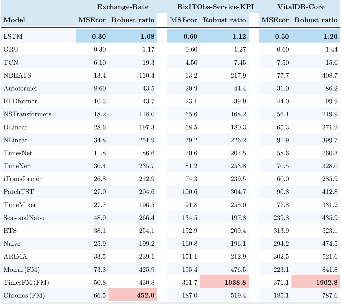
The added datasets were chosen to break the energy/climate monoculture of the original release, not to make the benchmark easier. They do not change the verdict.
| Model | 6-dataset r | Exchange-Rate | BizITObs | VitalDB |
|---|---|---|---|---|
| Naive | 105.7 | 199.2 | 196.1 | 474.5 |
| SeasonalNaive | 165.5 | 266.4 | 197.8 | 435.9 |
| ARIMA | 120.7 | 239.1 | 212.9 | 521.6 |
| ETS | 122.9 | 254.1 | 209.4 | 523.1 |
| DLinear | 197.3 | 197.3 | 180.3 | 271.9 |
| NLinear | 142.1 | 251.9 | 226.2 | 399.7 |
| N-BEATS | 54.6 | 110.4 | 217.9 | 408.7 |
| LSTM | 1.07 | 1.08 | 1.12 | 1.20 |
| GRU | 1.14 | 1.17 | 1.27 | 1.44 |
| TCN | 7.89 | 19.3 | 7.45 | 15.6 |
| Autoformer | 48.0 | 43.5 | 44.4 | 86.2 |
| FEDformer | 22.6 | 43.7 | 39.9 | 99.9 |
| PatchTST | 262.6 | 204.6 | 304.7 | 412.8 |
| iTransformer | 272.3 | 212.9 | 239.5 | 285.9 |
| TimeXer | 301.2 | 235.7 | 253.8 | 328.0 |
| TimeMixer | 264.2 | 196.5 | 255.0 | 331.2 |
| TimesNet | 141.7 | 86.6 | 207.5 | 260.3 |
| Nonstationary-Transformer | 101.1 | 118.0 | 168.2 | 219.9 |
| TimesFM (FM) | 555.2 | 430.8 | 1,038.8 | 1,902.8 |
| Chronos (FM) | 512.5 | 452.0 | 519.4 | 787.6 |
| Moirai (FM) | 365.6 | 425.9 | 476.5 | 841.8 |
Which mechanism dominates depends on the domain — and it depends on it in the direction the taxonomy predicts.
| Dataset | #Ch. | Mode I | Mode II | Mode III | Mode IV | IV / III |
|---|---|---|---|---|---|---|
| ETT (mean of four) | 7 | 1.075 | 1.047 | 361.1 | 135.4 | 0.375 |
| Weather | 21 | 1.083 | 1.001 | 124.6 | 14.8 | 0.119 |
| Electricity | 321 | 1.364 | 1.005 | 2,229.4 | 21.2 | 0.009 |
| Exchange-Rate | 8 | 1.12 | 1.07 | 680 | 80 | 0.118 |
| BizITObs-Service-KPI | 72 | 1.18 | 1.03 | 835 | 115 | 0.138 |
| VitalDB-Core | 8 | 1.26 | 1.02 | 1,490 | 145 | 0.097 |
(mean r over the 21 models, averaged across the five severities)
Four follow-up studies run on top of the same released grid. Each has its own driver script and its own results CSV, so every number below can be recomputed without touching the main pipeline.
Real incidents rarely arrive one at a time. Because the four modes are operators, they compose: TΘ = TΘ_B ∘ TΘ_A (Eq. 19). Both operators act on the same critical window W★, each keeps its own Θ, and at every severity the two constituents are matched at the same nominal difficulty, κ_A(Θ_A) = κ_B(Θ_B) = δ_s. One fixed application order per pair — composition is not commutative, so the order is itself a scenario parameter.
python compose_faults.py \
    --pairs I+II I+III I+IV II+III II+IV III+IV \
    --npz_root ./TS-Fault_output --out ./results_compound.csv
The amplification factor Ψ(A∘B) = r(A∘B) / max(r_A, r_B) asks whether a compound fault is worse than its more damaging half.
| Composition | Mean r | Ψ |
|---|---|---|
| single-mode reference: Mode I | 1.12 | — |
| single-mode reference: Mode II | 1.03 | — |
| single-mode reference: Mode III | 618.1 | — |
| single-mode reference: Mode IV | 97.1 | — |
| I ∘ II | 1.24 | 1.11 |
| II ∘ IV | 103.8 | 1.07 |
| I ∘ IV | 118.7 | 1.22 |
| II ∘ III | 763.4 | 1.24 |
| I ∘ III | 1,047.6 | 1.69 |
| III ∘ IV | 2,183.7 | 3.53 |
Ψ ≥ 1.07 — a compound fault is never easier than its worse half.Ψ = 3.53: a regime switch that a cascade then propagates is more than three times worse than either alone.r = 1.24. The stratification of Finding 2 survives composition — it is not an artifact of testing one mode at a time.S(W) doing any work?S(W) is the claim that a benchmark should stress the window a model relies on. If placement did not matter, TS-Fault would be a noise test with extra steps. We compare three placement policies at severity s₃ (d06), over 9 datasets × 21 models × 5 seeds, with random placement δ-matched so only the location differs:
python ablation_placement.py --policy topk random anti --severity d06 --seeds 5 \
    --out ./results_placement.csv
| Mode | Placement | Median RD (%) | Mean r | Catastrophic cells (%) | Seed IQR / median | ρ(clean, faulted) |
|---|---|---|---|---|---|---|
| I | Anti-selected | 0.43 | 1.009 | 0.0 | 1.37 | +0.999 |
| I | Random | 1.47 | 1.035 | 0.0 | 1.18 | +0.996 |
| I | Top-K S(W) | 5.11 | 1.110 | 0.0 | 0.27 | +0.983 |
| II | Anti-selected | 0.012 | 1.001 | 0.0 | 1.63 | +1.000 |
| II | Random | 0.034 | 1.004 | 0.0 | 1.46 | +0.999 |
| II | Top-K S(W) | 0.11 | 1.010 | 0.0 | 0.34 | +0.999 |
| III | Anti-selected | 9,872 | 216.4 | 62.7 | 1.08 | +0.286 |
| III | Random (δ-matched) | 18,436 | 398.7 | 75.4 | 0.84 | +0.147 |
| III | Top-K S(W) | 26,232 | 560.9 | 88.8 | 0.31 | +0.023 |
| IV | Anti-selected | 684 | 13.7 | 38.1 | 1.21 | +0.374 |
| IV | Random (δ-matched) | 1,536 | 29.4 | 58.7 | 0.91 | +0.218 |
| IV | Top-K S(W) | 2,878 | 52.7 | 72.8 | 0.29 | +0.082 |
Anti-selected < Random < Top-K in every mode, on both metrics. Two consequences beyond "the score works": importance-based placement cuts seed-to-seed variability by 3–4× (the IQR/median column), so a given robustness number means something; and as placement is weakened the faulted ranking drifts back toward the clean ranking (Mode III ρ: 0.023 → 0.147 → 0.286). Random placement would have partially hidden the model-selection risk that motivates the benchmark.
S(W) weightsThe per-mode weights and window hyperparameters, in full:
| Mode | λ₁ (S_cp) | λ₂ (S_per) | λ₃ (S_var) | λ₄ (S_pred) | top-K | |W| | σ_p |
|---|---|---|---|---|---|---|---|
| I · Time-Warped Shock | 0.15 | 0.15 | 0.35 | 0.35 | 5 | 24 | 0.15P |
| II · Dependency Fracture | 0.15 | 0.20 | 0.25 | 0.40 | 5 | 24 | 0.15P |
| III · Regime Missingness | 0.40 | 0.25 | 0.15 | 0.20 | 5 | 24 | 0.15P |
| IV · Sensor-to-System Cascade | 0.20 | 0.15 | 0.30 | 0.35 | 5 | 24 | 0.15P |
One-at-a-time perturbation at severity s₃ (ablation_lambda.py):
| Mode | Perturbation | Δ median RD | ρ vs. default ranking |
|---|---|---|---|
| I | λ₃ × 0.5 | −18.7% | 0.958 |
| I | λ₃ × 2 | +12.6% | 0.964 |
| I | λ₄ → 0 | −43.8% | 0.890 |
| I | λ₁ → 0 | +1.9% | 0.982 |
| II | λ₄ → 0 | −51.4% | 0.871 |
| II | λ₂ × 2 | −3.7% | 0.969 |
| III | λ₁ × 0.5 | −29.6% | 0.934 |
| III | λ₁ → 0 | −54.2% | 0.877 |
| III | λ₃ × 2 | +6.8% | 0.969 |
| IV | λ₄ → 0 | −41.9% | 0.884 |
| IV | λ₂ → 0 | −2.3% | 0.979 |
The weight each mode is designed around is the one that matters: zeroing λ₄ (occlusion) costs 42–51% of the degradation in Modes I/II/IV, and zeroing λ₁ (change-point) costs 54% in Mode III. Removing a weight the mode does not emphasise moves the result by at most 2.3%. Crucially, the model ranking is stable throughout (ρ ≥ 0.871): the weights control how hard the benchmark is, not who wins.
The zero-shot fragility result invites the obvious question. We adapted all three foundation models under four settings and re-ran the full grid:
| Setting | What is trained | Evaluated on |
|---|---|---|
| ZS | nothing — released weights | full grid |
| LP | forecasting head only, clean data | full grid |
| FT | all parameters, clean data | full grid |
| FT-fault | all parameters, low-severity faulted data (s₁–s₂) | held-out severities s₃–s₅ |
python adapt_foundation.py --model timesfm --setting ft_fault \
    --train_severities d02 d04 --eval_severities d06 d08 d10 \
    --out ./results_foundation_adapt.csv
| Model | Setting | Clean MSE | Faulted MSE | ΔMSE | AVG r | Mode III r | Mode IV r | WC r |
|---|---|---|---|---|---|---|---|---|
| TimesFM | ZS | 0.516 | 162.7 | 162.2 | 555 | 2,013 | 205 | 4,073 |
| TimesFM | LP | 0.468 | 108.7 | 108.2 | 344.5 | 1,248 | 128.0 | 2,687 |
| TimesFM | FT | 0.378 | 58.3 | 57.9 | 182.6 | 654 | 74.2 | 1,426 |
| TimesFM | FT-fault | 0.412 | 6.78 | 6.37 | 12.2 | 38.7 | 8.24 | 76.5 |
| Chronos | ZS | 0.613 | 165.6 | 165.0 | 513 | 1,839 | 209 | 3,745 |
| Chronos | LP | 0.548 | 119.4 | 118.9 | 339.5 | 1,217 | 139.0 | 2,468 |
| Chronos | FT | 0.437 | 64.8 | 64.4 | 188.1 | 672 | 78.5 | 1,384 |
| Chronos | FT-fault | 0.479 | 8.36 | 7.88 | 14.3 | 46.2 | 9.13 | 91.7 |
| Moirai | ZS | 0.682 | 153.1 | 152.4 | 366 | 1,296 | 164 | 2,544 |
| Moirai | LP | 0.596 | 89.7 | 89.1 | 214.4 | 768 | 87.6 | 1,538 |
| Moirai | FT | 0.462 | 43.6 | 43.1 | 109.9 | 392 | 45.4 | 814 |
| Moirai | FT-fault | 0.507 | 5.92 | 5.41 | 9.74 | 30.8 | 6.17 | 55.4 |
| (reference) LSTM | trained | 0.733 | 0.780 | 0.047 | 1.07 | 1.17 | 1.10 | 1.25 |
s₃–s₅ during adaptation, so this is generalisation along κ, not memorisation of a severity.r = 9.74) is still ~9× less robust than a plain trained LSTM (r = 1.07). The accurate-and-robust quadrant remains empty.Average risk (AVG) describes typical behavior over the released fault grid; worst-case risk (WC) asks for the most damaging released configuration:
$$ \mathrm{WC}(f,\mathcal F)=\sup_{\Theta\in\Phi}\mathbb E[\ell\mid\Theta]. $$
We report two complementary quantities:
r — within each dataset, the maximum configuration-level robustness ratio, then averaged across the datasets. This uses the same within-dataset-then-average convention as AVG r, so the two columns are directly comparable.Worst-case risk over all four modes. WC/AVG is the ratio between the worst-case and average robustness risks.
| Model | Clean MSE | AVG MSE | WC MSE | AVG r | WC r | WC/AVG | WC attained at |
|---|---|---|---|---|---|---|---|
| Naive | 1.238 | 129 | 1,377 | 106 | 644 | 6.1× | Electricity / III / d10 |
| SeasonalNaive | 0.905 | 119 | 1,270 | 166 | 1,121 | 6.8× | Electricity / III / d10 |
| ARIMA | 0.999 | 122 | 1,069 | 121 | 695 | 5.8× | ETTh1 / III / d10 |
| ETS | 1.044 | 127 | 1,352 | 123 | 754 | 6.1× | Electricity / III / d10 |
| DLinear | 0.562 | 66.8 | 675 | 197 | 1,374 | 7.0× | Electricity / III / d10 |
| NLinear | 0.540 | 72.2 | 644 | 142 | 826 | 5.8× | ETTh1 / III / d10 |
| N-BEATS | 0.449 | 21.6 | 564 | 54.6 | 368 | 6.7× | Electricity / III / d10 |
| LSTM | 0.733 | 0.78 | 1.04 | 1.07 | 1.25 | 1.2× | ETTh1 / III / d10 |
| GRU | 0.680 | 0.77 | 1.19 | 1.14 | 1.50 | 1.3× | ETTh1 / IV / d10 |
| TCN | 0.874 | 7.39 | 138 | 7.89 | 61.4 | 7.8× | Electricity / III / d08 |
| Autoformer | 0.822 | 24.2 | 264 | 48.0 | 321 | 6.7× | Electricity / III / d10 |
| FEDformer | 1.072 | 24.3 | 258 | 22.6 | 135 | 6.0× | Electricity / III / d10 |
| PatchTST | 0.551 | 86.6 | 919 | 263 | 1,863 | 7.1× | Electricity / III / d10 |
| iTransformer | 0.529 | 83.2 | 905 | 272 | 2,008 | 7.4× | Electricity / III / d10 |
| TimeXer | 0.537 | 88.0 | 1,085 | 301 | 2,170 | 7.2× | Electricity / III / d10 |
| TimeMixer | 0.590 | 90.1 | 889 | 264 | 1,859 | 7.0× | Electricity / III / d10 |
| TimesNet | 0.571 | 53.3 | 500 | 142 | 964 | 6.8× | Electricity / III / d10 |
| NS Transformer | 0.608 | 55.2 | 571 | 101 | 635 | 6.3× | Electricity / III / d10 |
| TimesFM | 0.516 | 163 | 1,746 | 555 | 4,073 | 7.3× | Electricity / III / d10 |
| Chronos | 0.613 | 166 | 1,757 | 513 | 3,745 | 7.3× | Electricity / III / d10 |
| Moirai | 0.682 | 153 | 1,530 | 366 | 2,544 | 7.0× | Electricity / III / d10 |
Per-mode worst-case risk. Each cell reports WC r / WC MSE.
| Model | Mode I | Mode II | Mode III | Mode IV |
|---|---|---|---|---|
| Naive | 1.04 / 2.07 | 1.00 / 2.01 | 644 / 1,377 | 285 / 508 |
| SeasonalNaive | 1.46 / 2.36 | 1.17 / 2.23 | 1,121 / 1,270 | 303 / 455 |
| ARIMA | 1.10 / 1.60 | 1.02 / 1.47 | 695 / 1,069 | 376 / 509 |
| ETS | 1.06 / 1.70 | 1.00 / 1.63 | 754 / 1,352 | 327 / 499 |
| DLinear | 1.49 / 0.98 | 1.06 / 0.93 | 1,374 / 675 | 281 / 309 |
| NLinear | 1.47 / 1.00 | 1.24 / 1.00 | 826 / 644 | 390 / 364 |
| N-BEATS | 1.20 / 1.90 | 1.05 / 1.45 | 361 / 564 | 127 / 68.2 |
| LSTM | 1.00 / 0.91 | 1.00 / 0.91 | 1.23 / 1.04 | 1.17 / 1.01 |
| GRU | 1.01 / 0.88 | 1.00 / 0.87 | 1.41 / 1.13 | 1.40 / 1.19 |
| TCN | 1.00 / 1.05 | 1.01 / 1.08 | 60.8 / 138 | 16.9 / 67.4 |
| Autoformer | 1.26 / 1.23 | 1.14 / 1.21 | 321 / 264 | 57.2 / 104 |
| FEDformer | 1.07 / 1.51 | 1.05 / 1.44 | 135 / 258 | 50.8 / 106 |
| PatchTST | 1.52 / 1.29 | 1.24 / 1.02 | 1,863 / 919 | 372 / 349 |
| iTransformer | 1.58 / 1.01 | 1.12 / 0.90 | 2,008 / 905 | 403 / 341 |
| TimeXer | 1.45 / 1.04 | 1.08 / 0.96 | 2,170 / 1,085 | 380 / 325 |
| TimeMixer | 1.44 / 1.01 | 1.07 / 0.95 | 1,859 / 889 | 371 / 383 |
| TimesNet | 1.64 / 1.06 | 1.14 / 1.11 | 964 / 500 | 231 / 247 |
| NS Transformer | 1.62 / 1.12 | 1.61 / 1.79 | 627 / 571 | 286 / 304 |
| TimesFM | 1.33 / 0.98 | 1.08 / 1.06 | 4,073 / 1,746 | 561 / 575 |
| Chronos | 1.25 / 1.03 | 1.03 / 0.95 | 3,745 / 1,757 | 588 / 589 |
| Moirai | 1.19 / 1.21 | 1.03 / 1.18 | 2,544 / 1,530 | 464 / 556 |
Three conclusions follow:
d10; TCN is the sole exception, peaking at d08.WC r = 1.64 in Modes I/II, whereas 19 of 21 exceed WC r = 10 in both Modes III and IV. LSTM and GRU are the only exceptions.TS-Fault is designed to be fully reproducible. Because faulted instances are produced by an explicit operator at evaluation time, the benchmark can be regenerated at any severity by re-sweeping κ, and previously-unexposed Θ combinations can be held out at release time to guard against benchmark gaming. We release:
Θ schemas and the unified window-importance front-end — plus compose_faults.py for the compound-fault operator TΘ_B ∘ TΘ_A;λ and β values used by S(W) and κ in every mode, with the placement and weight ablations that probe them (ablation_placement.py, ablation_lambda.py);adapt_foundation.py for the LP / FT / FT-fault adaptation protocol;TS-Fault code is released under the MIT licence. Some baseline implementations are adapted from external sources and retain their own licences: TCN from locuslab/TCN (MIT), NLinear/DLinear from cure-lab/LTSF-Linear (Apache-2.0), and N-BEATS from ServiceNow/N-BEATS (CC-BY-NC-4.0, non-commercial). The eight Transformer baselines come from the Time-Series-Library. Datasets (ETT, Electricity, Weather) are released by their original authors under CC BY 4.0 and are not redistributed here.