The primary problem with LLMs is their tendency to generate hallucinations (content that is false, inconsistent with context, or entirely fabricated). This presents significant challenges, particularly in applications where reliability is crucial, such as healthcare, law, and education. The issue becomes even more pronounced in multilingual settings, where language nuances can further exacerbate inaccuracies.
The aim of this project is to develop a solution that accurately detects hallucination spans in the outputs of instruction-tuned LLMs across multiple languages. The goal is to create a system that is not only precise but also adaptable to various languages and scalable to handle diverse text outputs.
The dataset used for this project was the Mu-SHROOM dataset from SemEval-2025 Task-3. It is a multilingual, multi-model resource designed for detecting hallucination spans in text generated by LLMs.
In this milestone we created a structured pipeline that reads, processes, and formats text data in various languages. We used tools like Stanza for linguistic preprocessing and then stored the output in JSONL and CoNLL-U format. The custom functions used for preprocessing were defined in a separate file (utils\preprocessing_functions.py) to keep the main preprocessing script (preprocessing_ver2.py) more organized and readable.
First, we loaded JSONL files and organize them by language. Each file is processed based on the language code, making it easier to handle multilingual data separately and ensure each language is processed with the correct tools. For each language found in the data, we set up an NLP pipeline using Stanza, which adapts to the language's unique grammar and vocabulary. For each language, we processed both the input and output texts in each record to extract linguistic features, including word lemmas, part-of-speech tags, and dependency relations. We converted the preprocessed text into CoNLL-U format, which includes metadata for each sentence and annotations for each token. Finally, we saved the processed data in two ways: in separate files, where each language’s data is saved as individual JSONL and CoNLL-U files and in two combined files, one containing all training and one all validation preproccesed files (see preprocessed folder).
Initially, the test dataset was unavailable, and only the validation dataset was labeled. Therefore, we used the preprocessed file preprocessed/val_preprocessed/combined_data.jsonl, splitting it into 80% training, 10% validation, and 10% testing data, ensuring no data leakage by separating the splits based on indices. After early experiments revealed the need for more data, we leveraged OpenAI's API and the GPT-4o-mini model to auto-label the training dataset, generating hallucination spans. Processing without batch optimization took 1–2 hours, and the total cost remained under $2. The Intersection over Union (IoU score provided by the Mu-SHROOM organizers) on the validation dataset, compared to the manually labeled data points, was 0.38166996. The labeling process showed significant variation, highlighting the complexity and ambiguity of the defined objective.
In the second milestone, we built upon the data prepared in Milestone 1 to develop two baseline models aimed at detecting hallucinated spans in language model outputs. Initially, we analyzed the data and visualized the hallucinated spans alongside the token-level logits generated by the model (see analysis_hallucinations.ipynb).
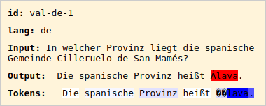 Figure 1: Labeled Hallucination Span (red) with lower token probabilities (blue).
An example of this visualization is shown in the accompanying figure. This analysis informed our decision to approach the task as a token-level classification problem, where each token is predicted to be either hallucinated or not.
To tackle this, we employed a dual-method approach. The first involves using a classical machine learning method, specifically variants of boosted random forests, leveraging only the token logits produced by the language model. The second combines this with an encoder-based fine-tuning approach to enhance the model's ability to identify hallucinated spans. This complementary strategy ensures a robust foundation for detecting hallucinations effectively.
The architecture of the model is illustrated in the overview diagram.
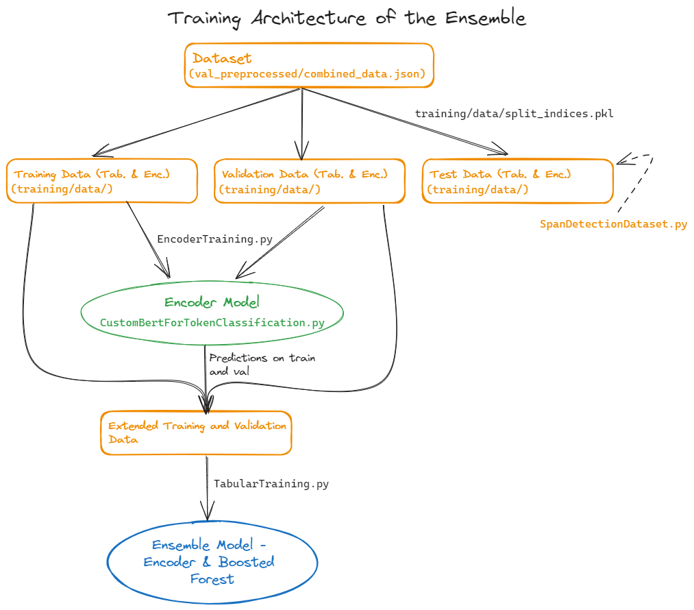 Figure 2: Model architecture overview - first training the encoder model which is then used as input in the tabular boosted forest model.
To streamline our workflow across both the tabular and encoder-based approaches, we consolidated the dataset preparation into a single class (SpanDetectionDataset.py). This class is designed to support both model types efficiently. The indices used during the encoder-based data preparation are carefully stored to ensure the same splits are applied when preparing data for the tabular model, maintaining consistency across approaches.
The training process begins with fine-tuning a BERT-based encoder model for token-level hallucination detection. This is implemented using a custom CustomBertForTokenClassification class, which extends BertPreTrainedModel by adding a binary classification head on top of BERT's contextualized embeddings. The model processes tokenized input sequences and predicts, for each token, whether it corresponds to a hallucination (1) or not (0).
For training, we utilize the BCEWithLogitsLoss function for binary classification and the AdamW optimizer with a learning rate of 5e-5 and a weight decay of 0.01. The model is trained for 15 epochs with early stopping based on validation loss, using a batch size of 8. To address memory limitations, we incorporate gradient accumulation with 2 steps to simulate larger batch sizes and employ mixed precision training (fp16) for improved memory efficiency.
The training process includes a warmup period of 10 steps and evaluates the model's performance after each epoch using metrics such as F1-score, precision, recall, and AUROC. This strategy enables the model to learn contextual patterns indicative of hallucinated content, leveraging the pre-trained language understanding capabilities of BERT.
After training the encoder-based model, its token-level predictions are used as additional features for boosted random forest models. Since boosted random forest models do not inherently learn features, we conducted extensive feature engineering, implemented in the FeatureEngineering class within the TabularTraining.py script.
A key feature is the cosine similarity between the model's input text and output text, as lower semantic similarity can indicate potential hallucinations in the output. Additionally, we drew inspiration from time-series analysis to engineer features. The FeatureEngineering class processes token-level data by computing basic statistics (mean, standard deviation, median, minimum, maximum, count) for each group (id). It also creates lagged and lead features within a specified window size (k_window), further calculating statistical measures and applying scaling transformations like min-max scaling and z-score normalization. This approach captures temporal patterns in token logits across sequences, making it well-suited for hallucination detection.
This feature engineering was applied to both the logits from the language model and the probabilities generated by the encoder-based model. The resulting dataset comprises 182 features, which may appear large relative to the limited initial SHROOMS dataset. However, converting the data into a tabular format, where each token represents a row, significantly expands the dataset: 31,062 rows for training, 4,264 for validation, and 5,097 for testing.
To identify the best-performing boosted random forest model, we utilized Optuna for hyperparameter optimization. We experimented with XGBoost, CatBoost, and LightGBM, as these algorithms inherently perform feature selection and require less pre-processing, allowing for more experimentation. One model per algorithm was trained and optimized based on evaluation metrics, including F1 score, precision, and recall. The best-performing models, along with their respective hyperparameters, were saved.
Additionally, we explored a two-stage ensemble approach to combine precision-optimized and recall-optimized models. In this setup, the recall-optimized model acts as a screener, identifying potential positive cases using a threshold. These candidates are then refined by the precision-optimized model for final classification. This ensemble method balances sensitivity and specificity, enhancing overall model performance.
To recreate the model using this repository (unfortunately, we cannot upload the entire model as the BERT-based encoder model is too large for Git), follow these steps:
requirements.txt or environment.yml file.model_training.py script, which trains the model with the specified parameters and saves it to the dedicacted folder (training by default).You can analyze the results using the model_analysis.ipynb notebook.
Our performance evaulation involves using standard binary classification metrics such as F1 score, precision, recall, accuracy, and AUROC. Additionally, we adopted the IOU and correlation scoring functions provided by the SHROOMS organizers.
In the subsequent sections, we will briefly discuss the metrics achieved during the training of the encoder-based model, followed by a performance comparison of the combined model. Detailed analyses and results can also be found in the model_analysis.ipynb script.
The performance plots highlight one of the most significant challenges we face: the limited amount of labeled data, particularly for the encoder-based model. This is evident from the erratic behavior of the training loss and the increasing validation loss, indicating that the model's performance on validation data deteriorates as training progresses. Consequently, the best encoder-based model was identified early, after just 6 epochs.
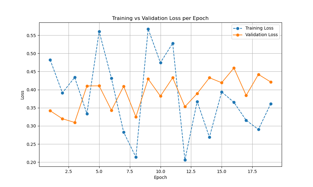 Figure 3: Training and Validation loss of the Encoder based model. Shows the lack of labeled training data.
Across all epochs, metrics such as accuracy and AUROC remain consistently high due to the class imbalance (hallucination vs. non-hallucination). However, the other metrics (e.g., F1 score, precision, recall) show a relatively stable performance, with a slight downward trend on the validation data as training continues for more epochs. This underscores the importance of addressing data limitations to improve the robustness of the models.
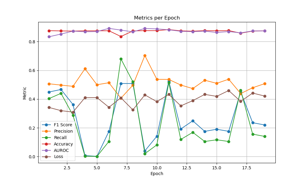 Figure 4: Performance Metrics per Epoch of the Encoder based model.
The ROC and PR curve plots reveal signs of overfitting on the training data, likely due to the large number of features created, the choice of algorithms, and insufficient regularization. Despite this, all models perform better than random guessing, demonstrating their ability to learn meaningful patterns. However, metrics such as precision and recall remain challenging across all models.
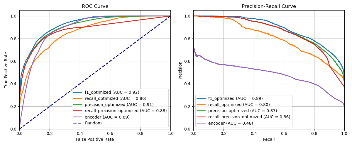 Figure 5.1: ROC and PR Curves on the training dataset for all models.
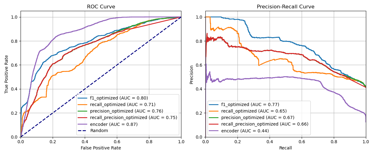 Figure 5.2: ROC and PR Curves on the validation dataset for all models.
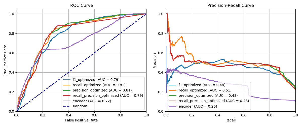 Figure 5.2: ROC and PR Curves on the testing dataset for all models.
One positive observation is that incorporating encoder predictions as inputs for the tabular model has proven successful in improving overall model performance. This indicates that the combined approach effectively leverages the strengths of both model types to enhance hallucination detection, this can also be seen in the below tables with ther performances on each of the datasets and the models used.
Training Dataset Performance:
| f1_optimized | recall_optimized | precision_optimized | recall_precision_optimized | encoder | |
|---|---|---|---|---|---|
| f1 | 0.764781 | 0.759363 | 0.743094 | 0.743807 | 0.500399 |
| precision | 0.808605 | 0.813979 | 0.803076 | 0.804979 | 0.620116 |
| recall | 0.725463 | 0.711615 | 0.691449 | 0.691276 | 0.419426 |
| accuracy | 0.834009 | 0.832239 | 0.822162 | 0.82287 | 0.895745 |
| auroc | 0.905971 | 0.907036 | 0.895644 | 0.877449 | 0.942409 |
Validation Dataset Performance:
| f1_optimized | recall_optimized | precision_optimized | recall_precision_optimized | encoder | |
|---|---|---|---|---|---|
| f1 | 0.642702 | 0.677715 | 0.623411 | 0.623577 | 0.299226 |
| precision | 0.70785 | 0.708101 | 0.758958 | 0.760621 | 0.459709 |
| recall | 0.588536 | 0.64983 | 0.528944 | 0.528377 | 0.221797 |
| accuracy | 0.729597 | 0.744606 | 0.735929 | 0.736398 | 0.870057 |
| auroc | 0.794706 | 0.805618 | 0.776839 | 0.791107 | 0.88516 |
Test Dataset Performance:
| f1_optimized | recall_optimized | precision_optimized | recall_precision_optimized | encoder | |
|---|---|---|---|---|---|
| f1 | 0.562311 | 0.464747 | 0.460668 | 0.459948 | 0.363458 |
| precision | 0.558219 | 0.542294 | 0.564232 | 0.567602 | 0.491042 |
| recall | 0.566464 | 0.406603 | 0.389227 | 0.38662 | 0.288499 |
| accuracy | 0.800863 | 0.788503 | 0.794193 | 0.794977 | 0.900735 |
| auroc | 0.781035 | 0.754222 | 0.739272 | 0.707529 | 0.711437 |
Here, we briefly discuss some challenges encountered with our approach. A primary difficulty lies in combining a model-agnostic approach (analyzing input and output text) with a token-level approach (utilizing model-specific logits and token-level predictions). As previously mentioned, this often results in inaccurate token mappings between the outputs of the language model and our encoder-based model, complicating the evaluation and scoring process.
IOU/Correlation could be effectively used as the metric during both encoder and tabular model training. However, due to these misalignments, we have not yet been able to fully implement this solution.
Auto-labeling could be improved by leveraging an ensemble of large language models with a voting mechanism, similar to the SHROOMS dataset creation process, which would generate more accurate probability estimates for the soft labels.
The primary problem with LLMs is their tendency to generate hallucinations (content that is false, inconsistent with context, or entirely fabricated). This presents significant challenges, particularly in applications where reliability is crucial, such as healthcare, law, and education. The issue becomes even more pronounced in multilingual settings, where language nuances can further exacerbate inaccuracies.
The aim of this project is to develop a solution that accurately detects hallucination spans in the outputs of instruction-tuned LLMs across multiple languages. The goal is to create a system that is not only precise but also adaptable to various languages and scalable to handle diverse text outputs.
The dataset used for this project was the Mu-SHROOM dataset from SemEval-2025 Task-3. It is a multilingual, multi-model resource designed for detecting hallucination spans in text generated by LLMs.
In this milestone we created a structured pipeline that reads, processes, and formats text data in various languages. We used tools like Stanza for linguistic preprocessing and then stored the output in JSONL and CoNLL-U format. The custom functions used for preprocessing were defined in a separate file (utils\preprocessing_functions.py) to keep the main preprocessing script (preprocessing_ver2.py) more organized and readable.
First, we loaded JSONL files and organize them by language. Each file is processed based on the language code, making it easier to handle multilingual data separately and ensure each language is processed with the correct tools. For each language found in the data, we set up an NLP pipeline using Stanza, which adapts to the language's unique grammar and vocabulary. For each language, we processed both the input and output texts in each record to extract linguistic features, including word lemmas, part-of-speech tags, and dependency relations. We converted the preprocessed text into CoNLL-U format, which includes metadata for each sentence and annotations for each token. Finally, we saved the processed data in two ways: in separate files, where each language’s data is saved as individual JSONL and CoNLL-U files and in two combined files, one containing all training and one all validation preproccesed files (see preprocessed folder).
Initially, the test dataset was unavailable, and only the validation dataset was labeled. Therefore, we used the preprocessed file preprocessed/val_preprocessed/combined_data.jsonl, splitting it into 80% training, 10% validation, and 10% testing data, ensuring no data leakage by separating the splits based on indices. After early experiments revealed the need for more data, we leveraged OpenAI's API and the GPT-4o-mini model to auto-label the training dataset, generating hallucination spans. Processing without batch optimization took 1–2 hours, and the total cost remained under $2. The Intersection over Union (IoU score provided by the Mu-SHROOM organizers) on the validation dataset, compared to the manually labeled data points, was 0.38166996. The labeling process showed significant variation, highlighting the complexity and ambiguity of the defined objective.
In the second milestone, we built upon the data prepared in Milestone 1 to develop two baseline models aimed at detecting hallucinated spans in language model outputs. Initially, we analyzed the data and visualized the hallucinated spans alongside the token-level logits generated by the model (see analysis_hallucinations.ipynb).
Figure 1: Labeled Hallucination Span (red) with lower token probabilities (blue).
An example of this visualization is shown in the accompanying figure. This analysis informed our decision to approach the task as a token-level classification problem, where each token is predicted to be either hallucinated or not.
To tackle this, we employed a dual-method approach. The first involves using a classical machine learning method, specifically variants of boosted random forests, leveraging only the token logits produced by the language model. The second combines this with an encoder-based fine-tuning approach to enhance the model's ability to identify hallucinated spans. This complementary strategy ensures a robust foundation for detecting hallucinations effectively.
The architecture of the model is illustrated in the overview diagram.
Figure 2: Model architecture overview - first training the encoder model which is then used as input in the tabular boosted forest model.
To streamline our workflow across both the tabular and encoder-based approaches, we consolidated the dataset preparation into a single class (SpanDetectionDataset.py). This class is designed to support both model types efficiently. The indices used during the encoder-based data preparation are carefully stored to ensure the same splits are applied when preparing data for the tabular model, maintaining consistency across approaches.
The training process begins with fine-tuning a BERT-based encoder model for token-level hallucination detection. This is implemented using a custom CustomBertForTokenClassification class, which extends BertPreTrainedModel by adding a binary classification head on top of BERT's contextualized embeddings. The model processes tokenized input sequences and predicts, for each token, whether it corresponds to a hallucination (1) or not (0).
For training, we utilize the BCEWithLogitsLoss function for binary classification and the AdamW optimizer with a learning rate of 5e-5 and a weight decay of 0.01. The model is trained for 15 epochs with early stopping based on validation loss, using a batch size of 8. To address memory limitations, we incorporate gradient accumulation with 2 steps to simulate larger batch sizes and employ mixed precision training (fp16) for improved memory efficiency.
The training process includes a warmup period of 10 steps and evaluates the model's performance after each epoch using metrics such as F1-score, precision, recall, and AUROC. This strategy enables the model to learn contextual patterns indicative of hallucinated content, leveraging the pre-trained language understanding capabilities of BERT.
After training the encoder-based model, its token-level predictions are used as additional features for boosted random forest models. Since boosted random forest models do not inherently learn features, we conducted extensive feature engineering, implemented in the FeatureEngineering class within the TabularTraining.py script.
A key feature is the cosine similarity between the model's input text and output text, as lower semantic similarity can indicate potential hallucinations in the output. Additionally, we drew inspiration from time-series analysis to engineer features. The FeatureEngineering class processes token-level data by computing basic statistics (mean, standard deviation, median, minimum, maximum, count) for each group (id). It also creates lagged and lead features within a specified window size (k_window), further calculating statistical measures and applying scaling transformations like min-max scaling and z-score normalization. This approach captures temporal patterns in token logits across sequences, making it well-suited for hallucination detection.
This feature engineering was applied to both the logits from the language model and the probabilities generated by the encoder-based model. The resulting dataset comprises 182 features, which may appear large relative to the limited initial SHROOMS dataset. However, converting the data into a tabular format, where each token represents a row, significantly expands the dataset: 31,062 rows for training, 4,264 for validation, and 5,097 for testing.
To identify the best-performing boosted random forest model, we utilized Optuna for hyperparameter optimization. We experimented with XGBoost, CatBoost, and LightGBM, as these algorithms inherently perform feature selection and require less pre-processing, allowing for more experimentation. One model per algorithm was trained and optimized based on evaluation metrics, including F1 score, precision, and recall. The best-performing models, along with their respective hyperparameters, were saved.
Additionally, we explored a two-stage ensemble approach to combine precision-optimized and recall-optimized models. In this setup, the recall-optimized model acts as a screener, identifying potential positive cases using a threshold. These candidates are then refined by the precision-optimized model for final classification. This ensemble method balances sensitivity and specificity, enhancing overall model performance.
To recreate the model using this repository (unfortunately, we cannot upload the entire model as the BERT-based encoder model is too large for Git), follow these steps:
requirements.txt or environment.yml file.model_training.py script, which trains the model with the specified parameters and saves it to the dedicacted folder (training by default).You can analyze the results using the model_analysis.ipynb notebook.
Our performance evaulation involves using standard binary classification metrics such as F1 score, precision, recall, accuracy, and AUROC. Additionally, we adopted the IOU and correlation scoring functions provided by the SHROOMS organizers.
In the subsequent sections, we will briefly discuss the metrics achieved during the training of the encoder-based model, followed by a performance comparison of the combined model. Detailed analyses and results can also be found in the model_analysis.ipynb script.
The performance plots highlight one of the most significant challenges we face: the limited amount of labeled data, particularly for the encoder-based model. This is evident from the erratic behavior of the training loss and the increasing validation loss, indicating that the model's performance on validation data deteriorates as training progresses. Consequently, the best encoder-based model was identified early, after just 6 epochs.
Figure 3: Training and Validation loss of the Encoder based model. Shows the lack of labeled training data.
Across all epochs, metrics such as accuracy and AUROC remain consistently high due to the class imbalance (hallucination vs. non-hallucination). However, the other metrics (e.g., F1 score, precision, recall) show a relatively stable performance, with a slight downward trend on the validation data as training continues for more epochs. This underscores the importance of addressing data limitations to improve the robustness of the models.
Figure 4: Performance Metrics per Epoch of the Encoder based model.
The ROC and PR curve plots reveal signs of overfitting on the training data, likely due to the large number of features created, the choice of algorithms, and insufficient regularization. Despite this, all models perform better than random guessing, demonstrating their ability to learn meaningful patterns. However, metrics such as precision and recall remain challenging across all models.
Figure 5.1: ROC and PR Curves on the training dataset for all models.
Figure 5.2: ROC and PR Curves on the validation dataset for all models.
Figure 5.2: ROC and PR Curves on the testing dataset for all models.
One positive observation is that incorporating encoder predictions as inputs for the tabular model has proven successful in improving overall model performance. This indicates that the combined approach effectively leverages the strengths of both model types to enhance hallucination detection, this can also be seen in the below tables with ther performances on each of the datasets and the models used.
Training Dataset Performance:
| f1_optimized | recall_optimized | precision_optimized | recall_precision_optimized | encoder | |
|---|---|---|---|---|---|
| f1 | 0.764781 | 0.759363 | 0.743094 | 0.743807 | 0.500399 |
| precision | 0.808605 | 0.813979 | 0.803076 | 0.804979 | 0.620116 |
| recall | 0.725463 | 0.711615 | 0.691449 | 0.691276 | 0.419426 |
| accuracy | 0.834009 | 0.832239 | 0.822162 | 0.82287 | 0.895745 |
| auroc | 0.905971 | 0.907036 | 0.895644 | 0.877449 | 0.942409 |
Validation Dataset Performance:
| f1_optimized | recall_optimized | precision_optimized | recall_precision_optimized | encoder | |
|---|---|---|---|---|---|
| f1 | 0.642702 | 0.677715 | 0.623411 | 0.623577 | 0.299226 |
| precision | 0.70785 | 0.708101 | 0.758958 | 0.760621 | 0.459709 |
| recall | 0.588536 | 0.64983 | 0.528944 | 0.528377 | 0.221797 |
| accuracy | 0.729597 | 0.744606 | 0.735929 | 0.736398 | 0.870057 |
| auroc | 0.794706 | 0.805618 | 0.776839 | 0.791107 | 0.88516 |
Test Dataset Performance:
| f1_optimized | recall_optimized | precision_optimized | recall_precision_optimized | encoder | |
|---|---|---|---|---|---|
| f1 | 0.562311 | 0.464747 | 0.460668 | 0.459948 | 0.363458 |
| precision | 0.558219 | 0.542294 | 0.564232 | 0.567602 | 0.491042 |
| recall | 0.566464 | 0.406603 | 0.389227 | 0.38662 | 0.288499 |
| accuracy | 0.800863 | 0.788503 | 0.794193 | 0.794977 | 0.900735 |
| auroc | 0.781035 | 0.754222 | 0.739272 | 0.707529 | 0.711437 |
Here, we briefly discuss some challenges encountered with our approach. A primary difficulty lies in combining a model-agnostic approach (analyzing input and output text) with a token-level approach (utilizing model-specific logits and token-level predictions). As previously mentioned, this often results in inaccurate token mappings between the outputs of the language model and our encoder-based model, complicating the evaluation and scoring process.
IOU/Correlation could be effectively used as the metric during both encoder and tabular model training. However, due to these misalignments, we have not yet been able to fully implement this solution.
Auto-labeling could be improved by leveraging an ensemble of large language models with a voting mechanism, similar to the SHROOMS dataset creation process, which would generate more accurate probability estimates for the soft labels.