Implementations of ML, using only numpy.
In the context of artificial neural networks:
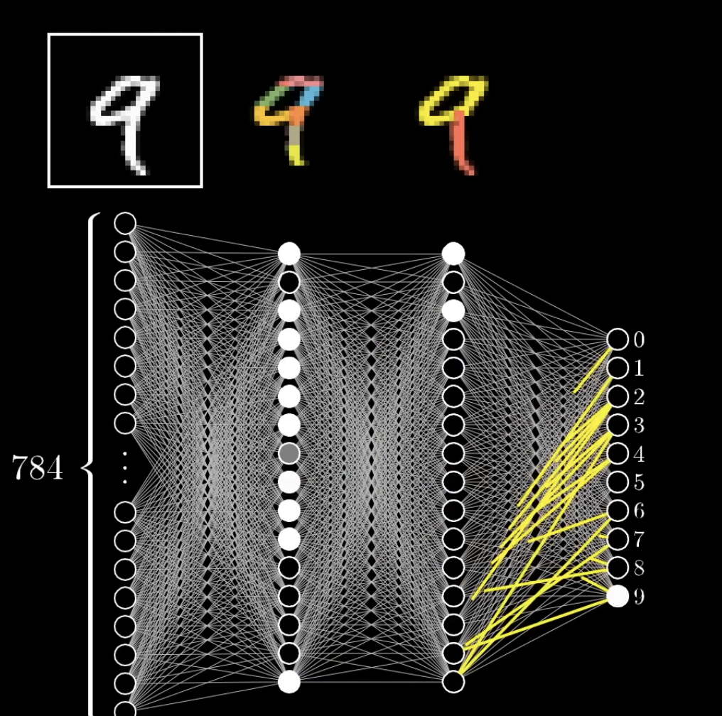
"weight"The activation of a neuron is calculated based on:
Here's how it works:
"bias"This can be represented by the formula:
weighted_sum = w1*a1 + w2*a2 + ... + wn*an + bias
Where:
w_i is the weight of the connection from neuron i in the previous layera_i is the activation of neuron i in the previous layer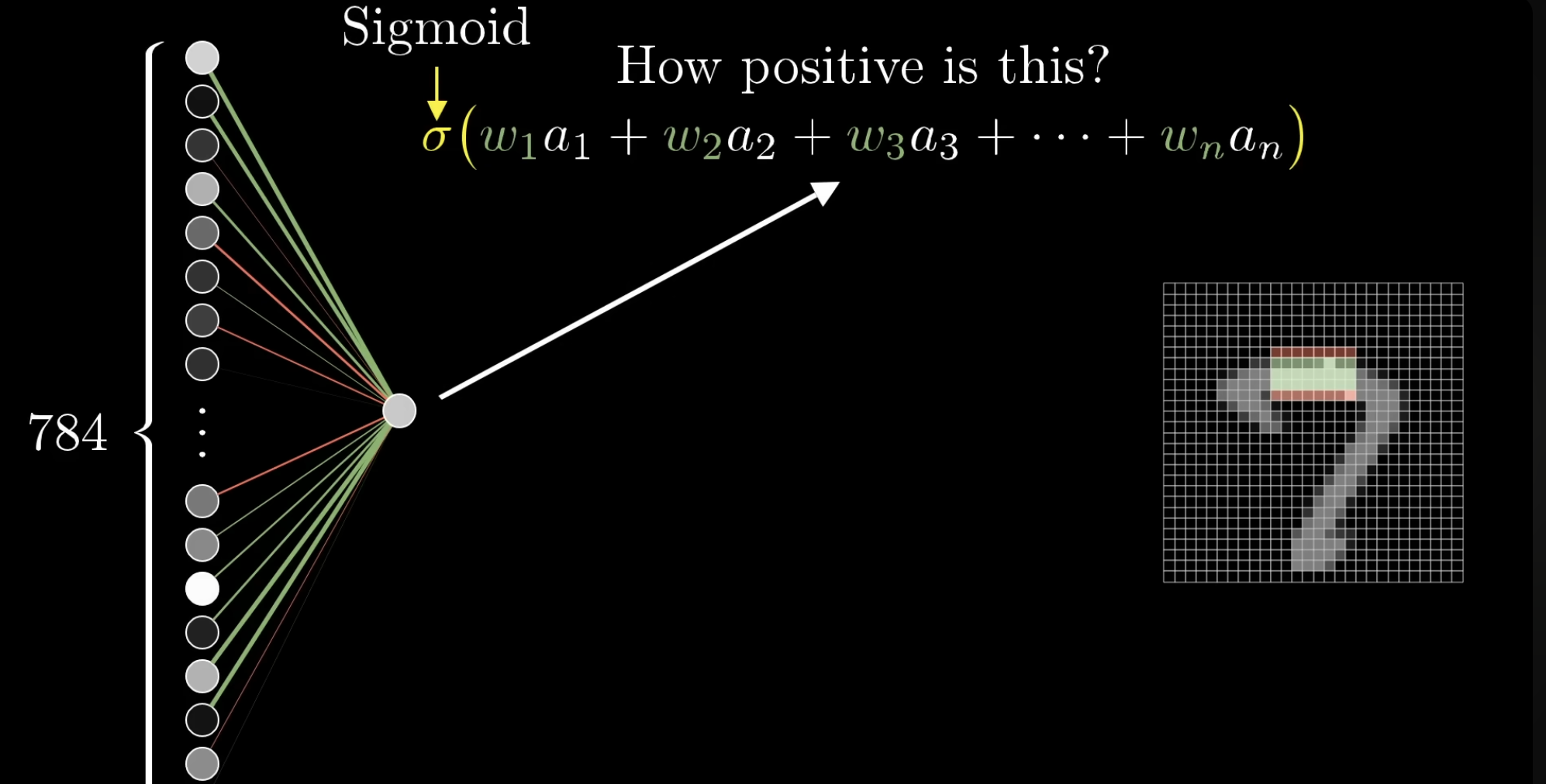
The bias shifts the activation function.
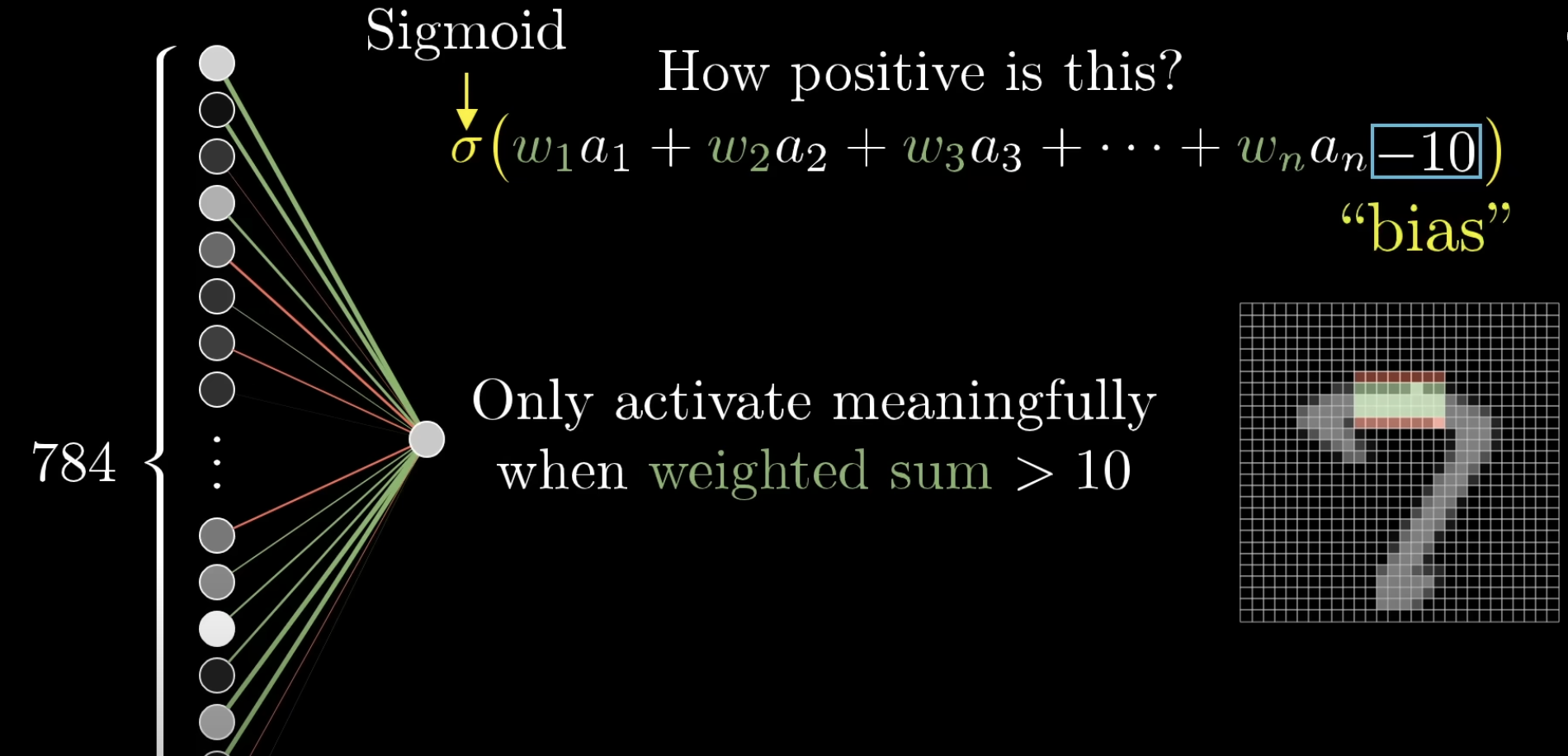
After calculating the weighted sum, we apply an "activation function". Common choices include:
In this guide, we'll focus on ReLU:
def relu(self, x):
        return np.maximum(0, x)
ReLU is popular because it helps the network learn more effectively.
Now that we understand the basic structure and operation of a neural network, let's look at how it learns.
This is the process of passing input through the network to get an output:
To train our network, we need to measure how well it's doing. We do this with a loss function:
The result is called the "loss".
def mse_loss(self, y, activations):
        return np.mean((activations-y)**2)
Thus, we aim to minimize the loss. We do this using:
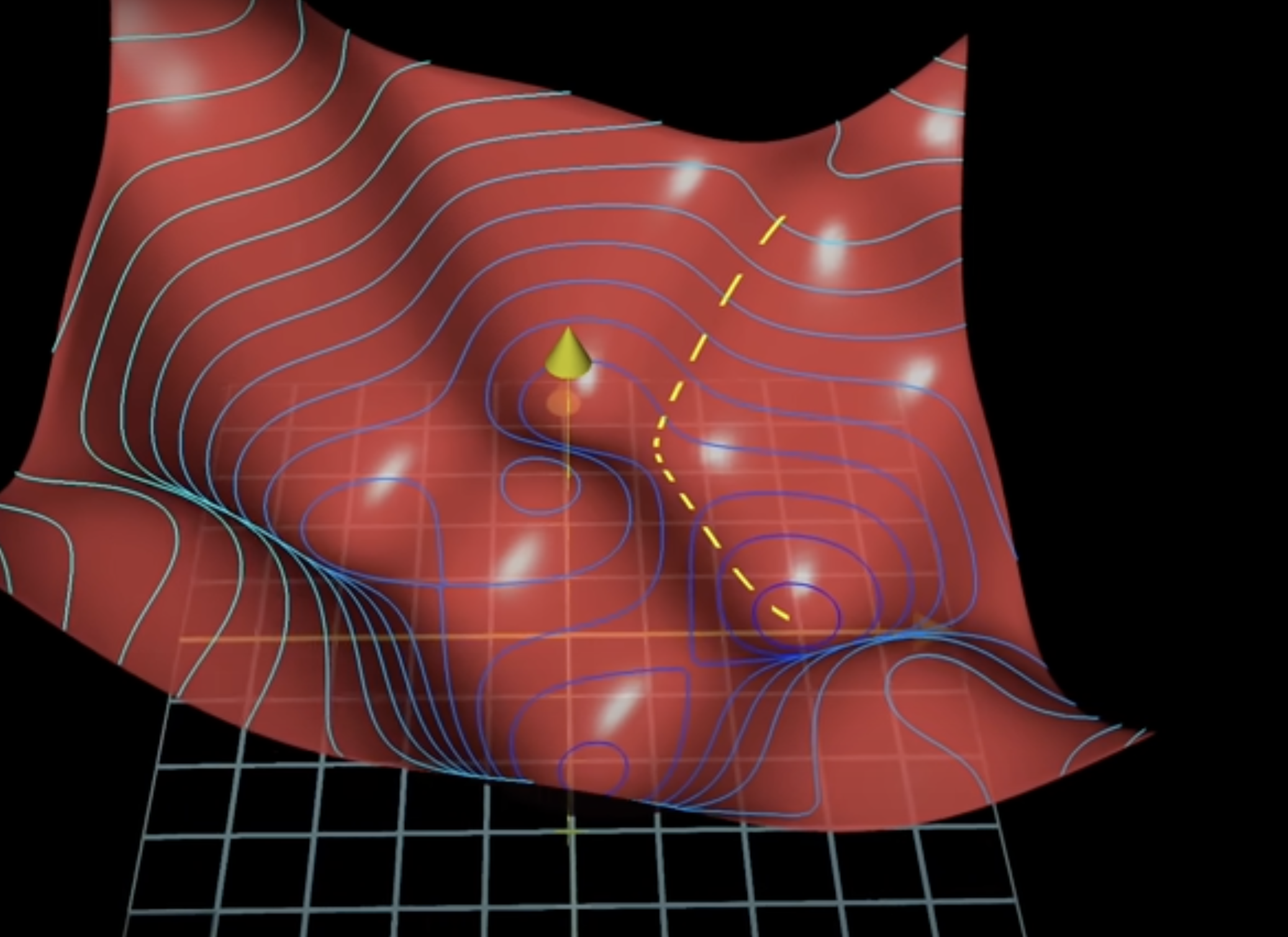
To improve the network's performance, i.e. minimize the loss, we need to adjust its weights and biases. We do this using two key concepts:
Here's how it works:
Optimization algorithm to minimize the loss function.
Uses gradients to update/adjust weights and biases in the direction that minimizes the loss.
We look for the negative gradient of the loss function, which tells us how we need to change the weights and biases to most efficiently decrease the loss
Backpropagation is the algorithm used to CALCULATE these gradients
The algorithm for determining how a SINGLE training example would like to nudge the weights and biases; not just if they should go up or down, but in terms of what relative proportions to those changes cause the most rapid decrease to the loss.
Activation is influenced in three ways:
w1*a1 + w2*a2 + ... + wn*an + bias
"Propagate backwards": backpropagation is applied in the direction from the last layer to the first layer.
------
∂C/∂w = ∂C/∂a × ∂a/∂z × ∂z/∂w
where C is loss/cost, w is weight, a is activation (output of neuron), z is the weighted sum (input to neuron, before activation).
This tells us how much the loss/cost (error) would change if we slightly adjusted a particular weight.
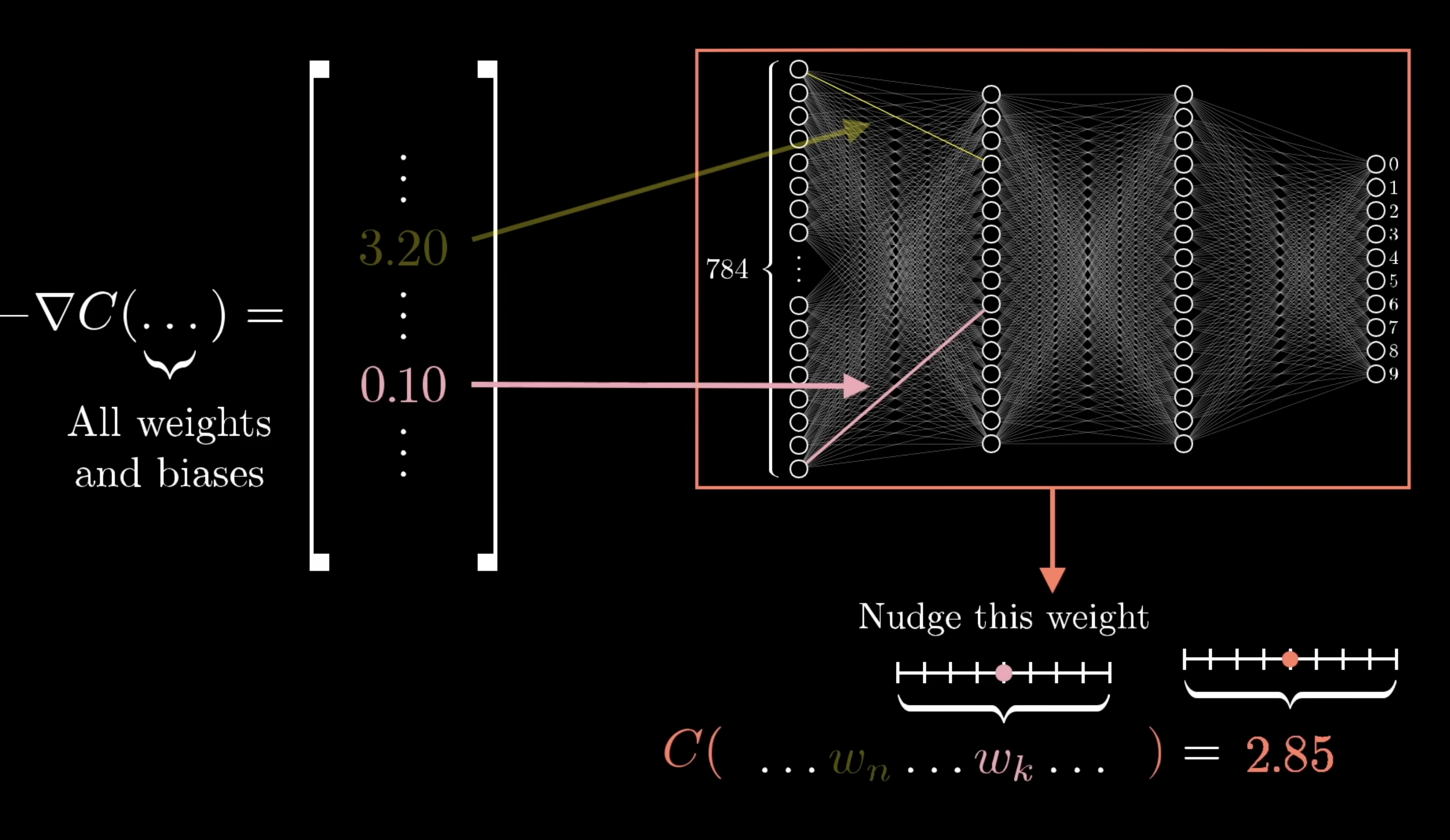
Averaged nudges to each weight and bias is the negative gradient of the loss function.
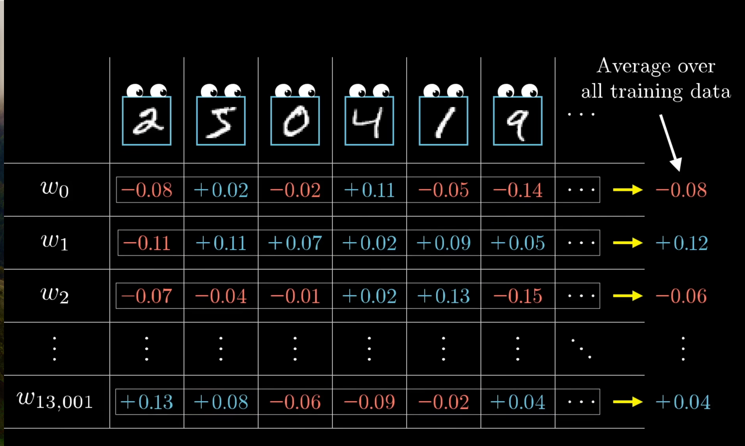
Training a neural network involves repeating these steps many times:
After many iterations, the network learns to recognize patterns in the training data and can apply this knowledge to new, unseen data.
For example: in digit recognition, each layer of the neural network can learn to detect common shapes (such as loops, curves, and vertical lines) that act as building blocks for recognizing all digits.
Here's a basic implementation of a neural network (feed-forward, multilayer percepton) from scratch in Python:
Manages multiple layers
Implements forward pass through all layers
Implements the training loop, including:
import numpy as np
import struct
import os
class Neuron:
    def __init__(self, num_inputs):
        self.weights = np.random.randn(num_inputs, 1) * 0.01
        self.bias = np.zeros((1, 1))
        self.last_input = None
        self.last_output = None

    def relu(self, z):
        return np.maximum(0, z)

    def relu_derivative(self, z):
        return np.where(z > 0, 1, 0)

    def forward(self, activations):
        self.last_input = activations
        z = np.dot(activations, self.weights) + self.bias
        self.last_output = self.relu(z)
        return self.last_output

    def backward(self, dC_da, learning_rate):
        da_dz = self.relu_derivative(self.last_output)
        dC_dz = dC_da * da_dz
        dC_dw = np.dot(self.last_input.T, dC_dz)
        dC_db = np.sum(dC_dz, axis=0, keepdims=True)

        self.weights -= learning_rate * dC_dw
        self.bias -= learning_rate * dC_db

        return np.dot(dC_dz, self.weights.T)


    # output_gradient:
        # A positive gradient means we need to decrease that output
        # A negative gradient means we need to increase that output

    # learning_rate: how big of a step is taken while updating weights and biases


class Layer:
    def __init__(self, num_neurons, num_inputs_per_neuron):
        self.neurons = [Neuron(num_inputs_per_neuron) for _ in range(num_neurons)]

    def forward(self, activations):
        return np.hstack([neuron.forward(activations) for neuron in self.neurons])

    def backward(self, output_gradient, learning_rate):
        return np.sum([neuron.backward(output_gradient[:, [i]], learning_rate) for i, neuron in enumerate(self.neurons)], axis=0)

class NeuralNetwork:
    def __init__(self, layer_sizes):
        self.layers = []
        for i in range(len(layer_sizes) - 1):
            self.layers.append(Layer(layer_sizes[i+1], layer_sizes[i]))

    def forward(self, activations):
        for layer in self.layers:
            activations = layer.forward(activations)
        return activations

    def mse_loss(self, y, activations):
        return np.mean((activations-y)**2)

    def derivative_mse_loss(self, y, activations):
        return 2*(activations-y) / y.shape[0]

    def train(self, X, y, epochs, learning_rate, batch_size=32):
        for epoch in range(epochs):
            total_loss = 0
            for i in range(0, len(X), batch_size):
                X_batch = X[i:i+batch_size]
                y_batch = y[i:i+batch_size]

                outputs = self.forward(X_batch)
                loss = self.mse_loss(y_batch, outputs)
                total_loss += loss * len(X_batch)

                output_gradient = self.derivative_mse_loss(y_batch, outputs)
                for layer in reversed(self.layers):
                    output_gradient = layer.backward(output_gradient, learning_rate)

            avg_loss = total_loss / len(X)
            print(f"Epoch {epoch+1}/{epochs}, Loss: {avg_loss}")

    def predict(self, X):
        return self.forward(X)
If you'd like a video format version, see the video below:
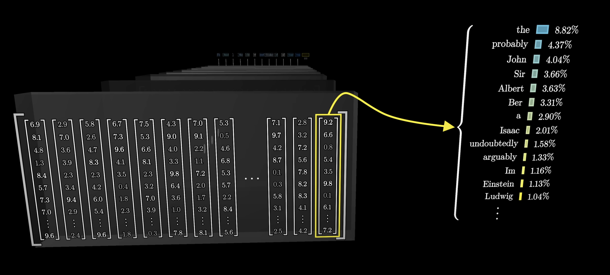
A collection of real numbers, which could be:
A probability distribution over all potential next tokens
Tokens are "little pieces" of information (ex. words, combinations of words, sounds, images)
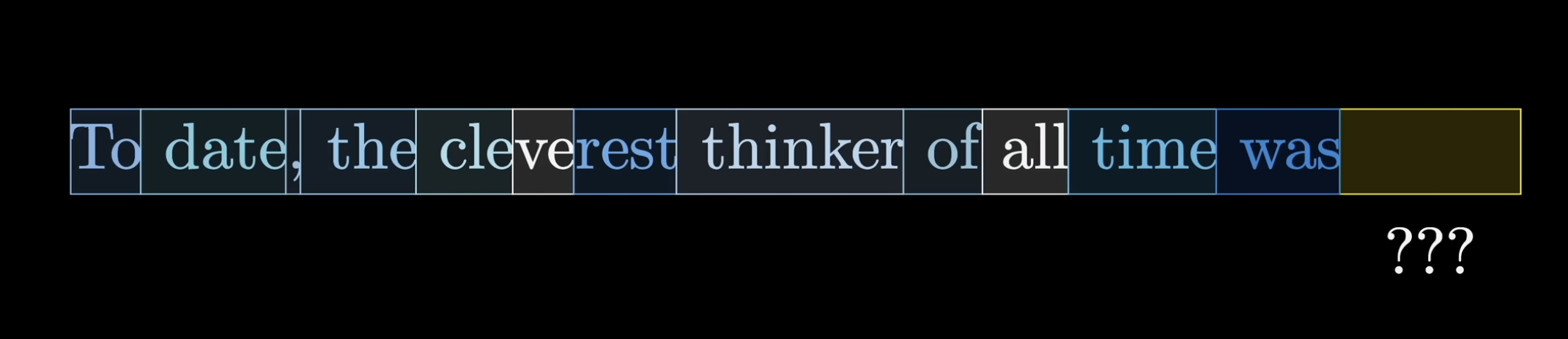
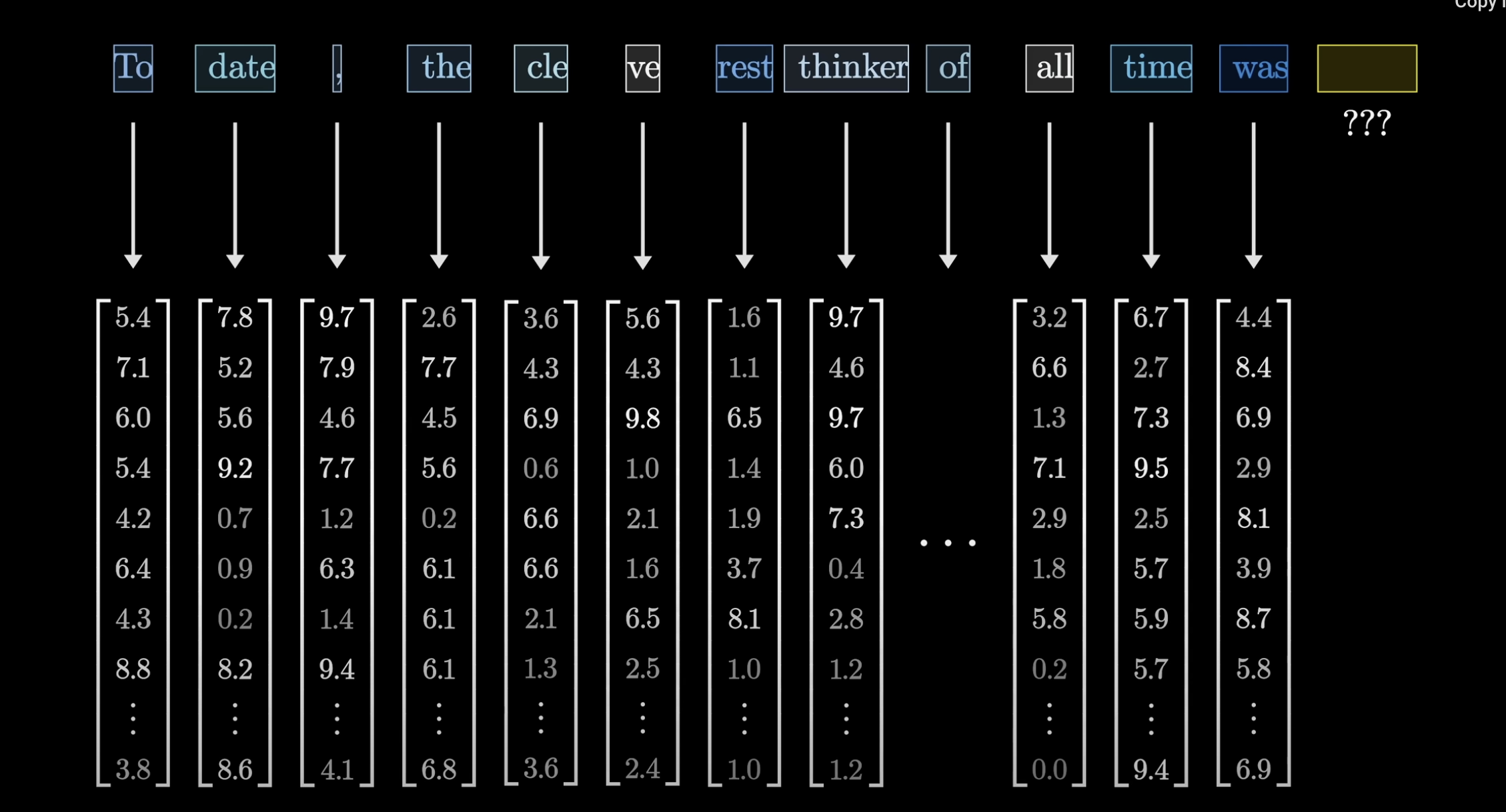
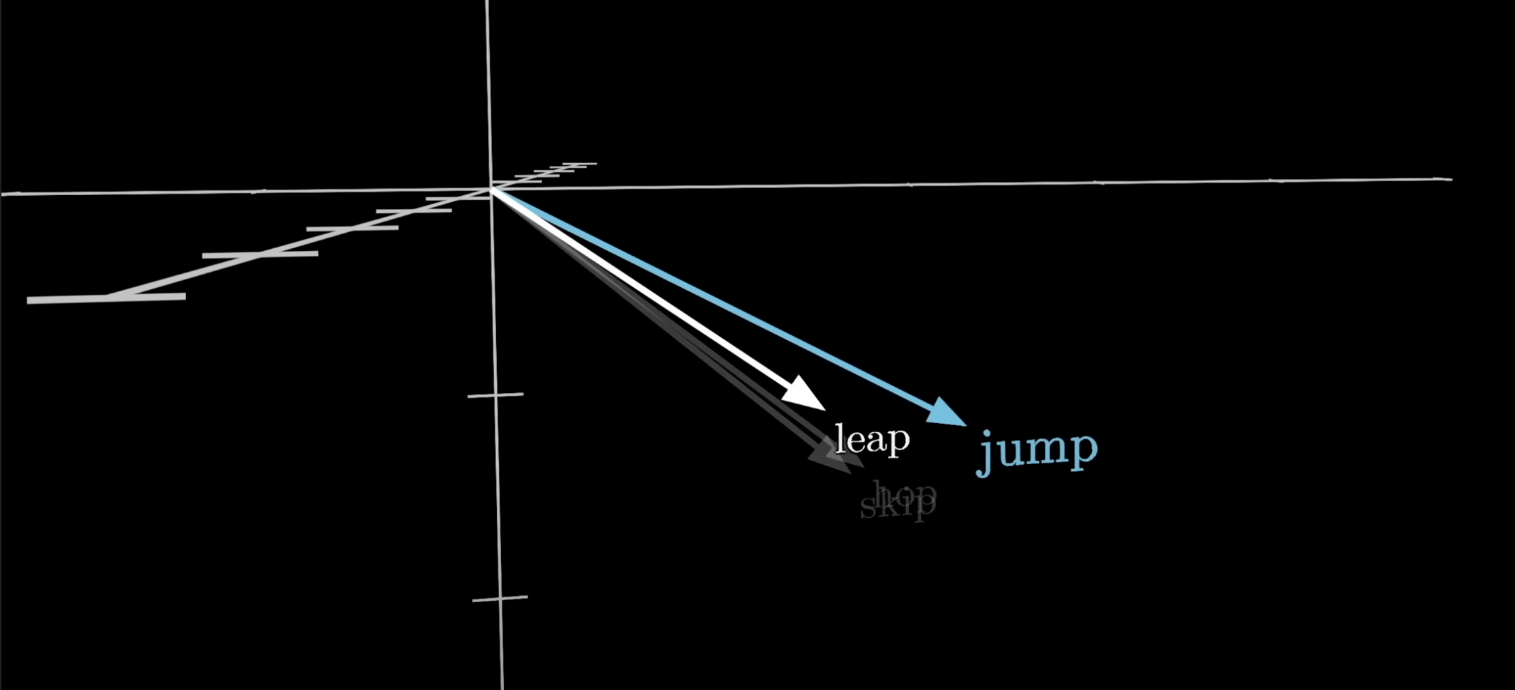
Words that are used and occur in the same context tend to purport similar meanings (distributional semantics)
See Transformer/embedding_notes.ipynb for more on embeddings!
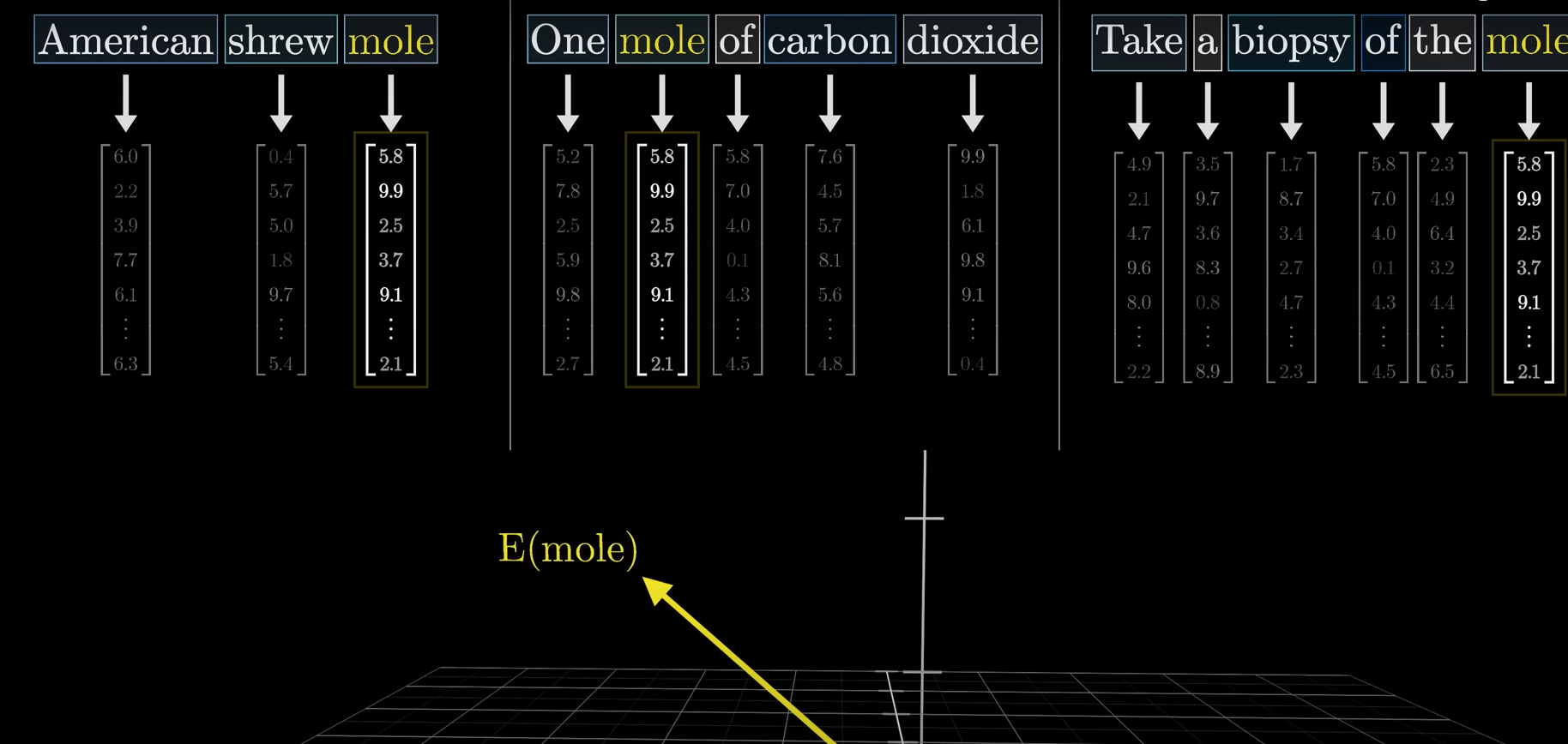
Below is an image of the embedding matrix. Each word corresponds to a specific vector, with no reference to its context. It is the Attention block's responsibility to update a word's vector with its context. (to be discussed later)
Positional encoding provides info about the order of tokens in a sequence.
NOTE: word embeddings & positional embeddings are separate. Word embeddings capture SEMANTIC MEANING, while positional encodings capture the ORDER of tokens
In determining desired output of the transformer (a probability distribution of all possible tokens that can come next in the generating text), a well trained network on the particular dataset is able to determine the next best possible token by:
The desired output of a transformer is a probability distribution of all possible tokens that can come next in the generating text
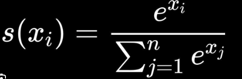
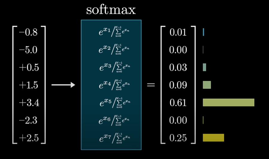
A probability distribution is defined as a sequence of numbers between 0-1, and that sums to 1. Softmax can give any sequence of numbers these criteria
import numpy as np

# given a sequence of numbers, each term `i`

# softmax eqn:      e^i/(sum of e^i for all terms)

# probability distribution:
    # 1) all numbers are positive numbers 0-1  (e^i)
    # sum of all numbers = 1 (sum of e^i of all terms)

seq = [2, 4, 5]
print(np.exp(seq)/np.sum(np.exp(seq)))
# [0.03511903 0.25949646 0.70538451]
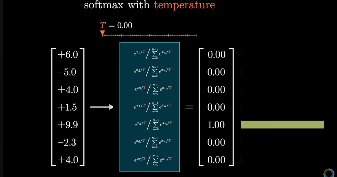
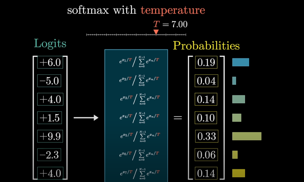
With softmax, the constant T added to the denominator of the exponents of e in the equation can cause more creative generated text
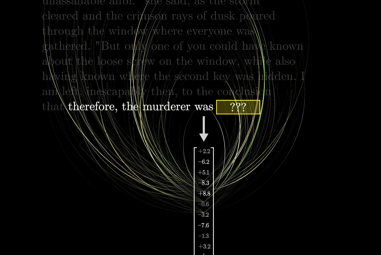
Goal: enable the model to focus on different parts of the input sequence when producing an output for a specific token
A value that represents how much focus (or attention) one word should give to another word in the sequence
(Its derivation is explained later)
Updates a word's embedding vector in reference to its context. Enables the transfer of information from one embedding to another
Prior to Attention, the embedding vector of each word is consistent, regardless of its context (embedding matrix). Therefore, the motivation of Attention is to update a word's embedding vector depending on its context (i.e. surrounding tokens) to capture this specific contextual instance of the word
The computation to predict the next token relies entirely on the final vector of the current sequence
Initially, this vector corresponds to the embedding of the last word in the sequence. As the sequence passes through the model's attention blocks, the final vector is updated to include information from the entire sequence, not just the last word. This updated vector becomes a summary of the whole sequence, encoding all the important information needed to predict the next word
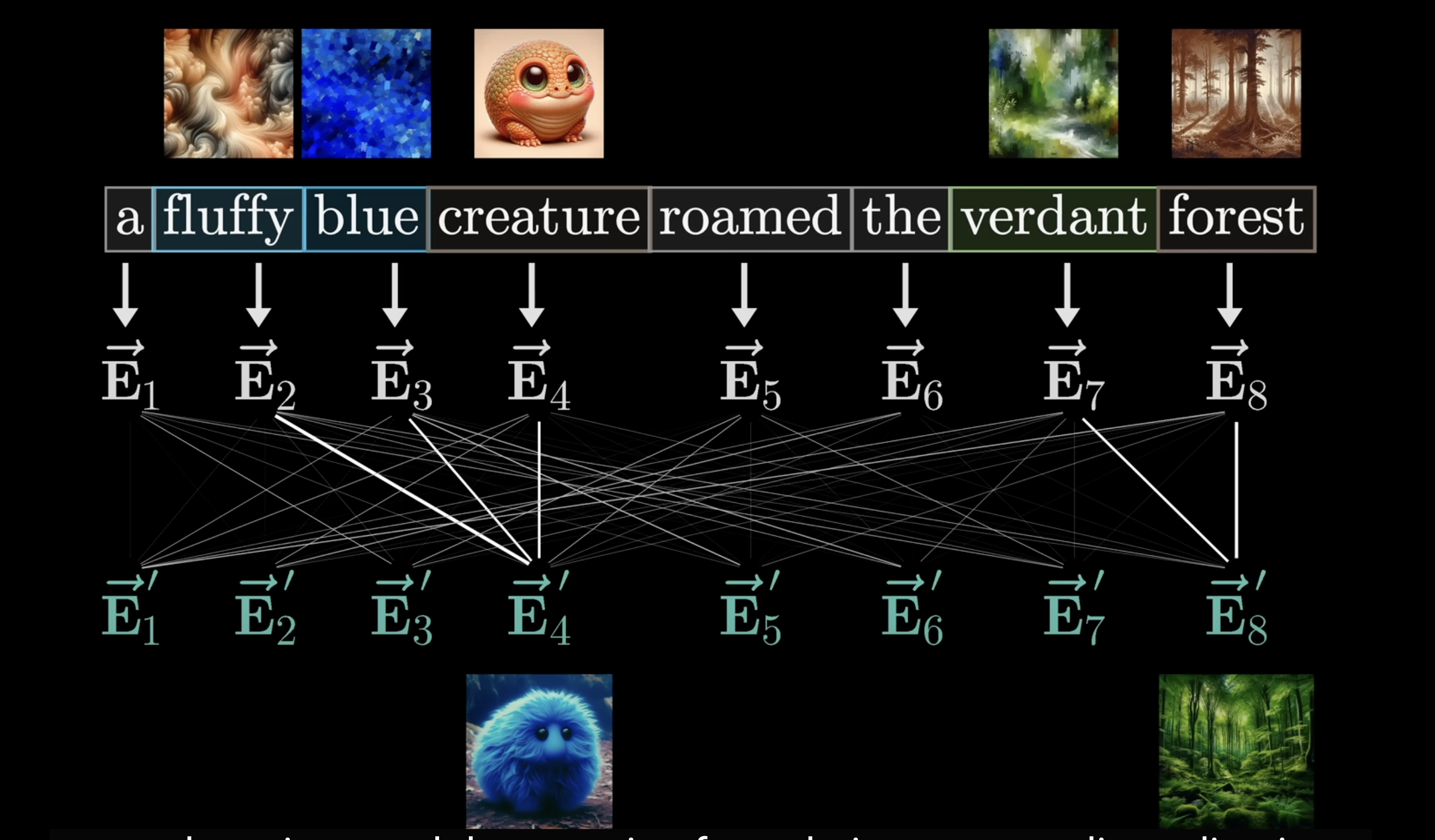
Goal: series of computations to produce a new refined set of embeddings
ex. Have nouns ingest the meanings of their corresponding adjectives
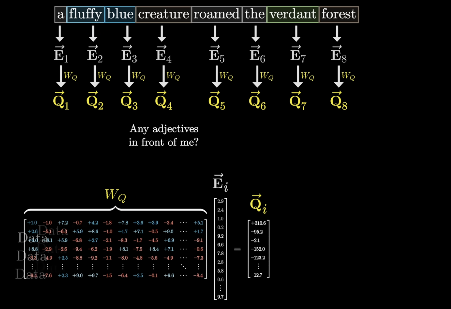
Query: represents the "question"/"focus" that the single-head attention is asking about the current word ex. if the current word is "cat" in the sentence "The cat sat on the mat", the Query for "cat" might be asking, "Which other words (Keys) in this sentence should I focus on to understand cat better?"
Key: serves as a criterion/reference point against which the Query is compared to determine the relevance of each word
Attention Score: tells us how relevant each word is
calculated as: the dot product between the Query and Key vectors
Input: Query, Key and Value matrices
Output: matrix where each vector is the weighted sum of the Value vectors, where the weights come from the attention scores (which are based on the dot product of the Query and Key matrices)
Steps:
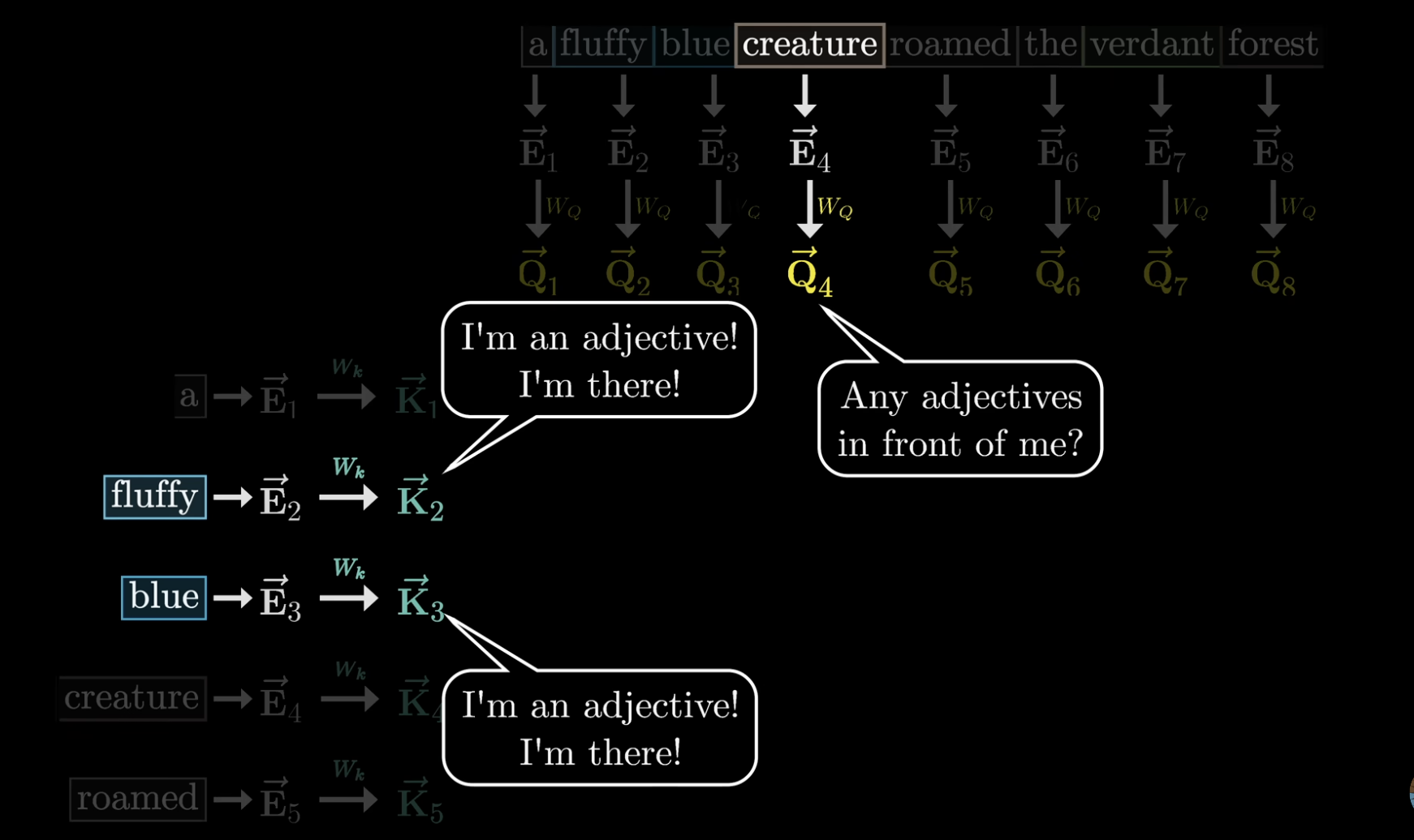
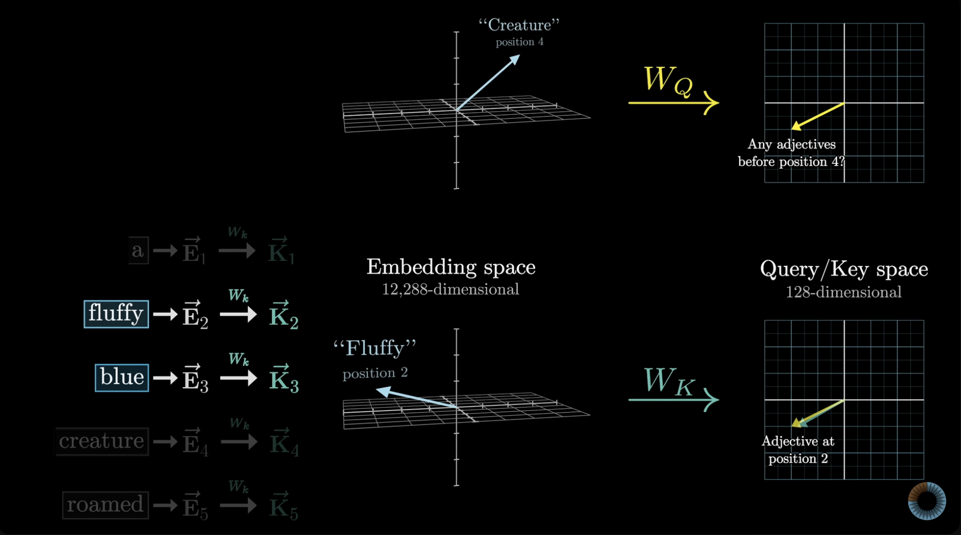
The higher the dot product, the more relevant the Query to the Key (i.e. word to another word in the sentence)
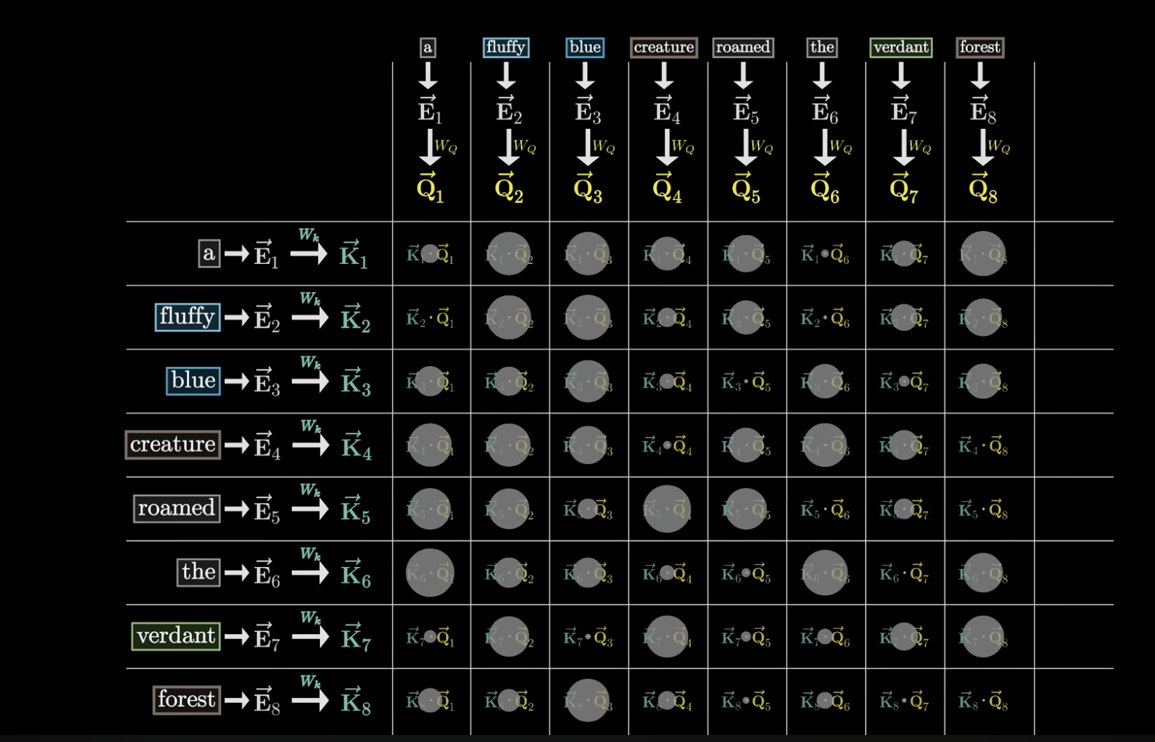
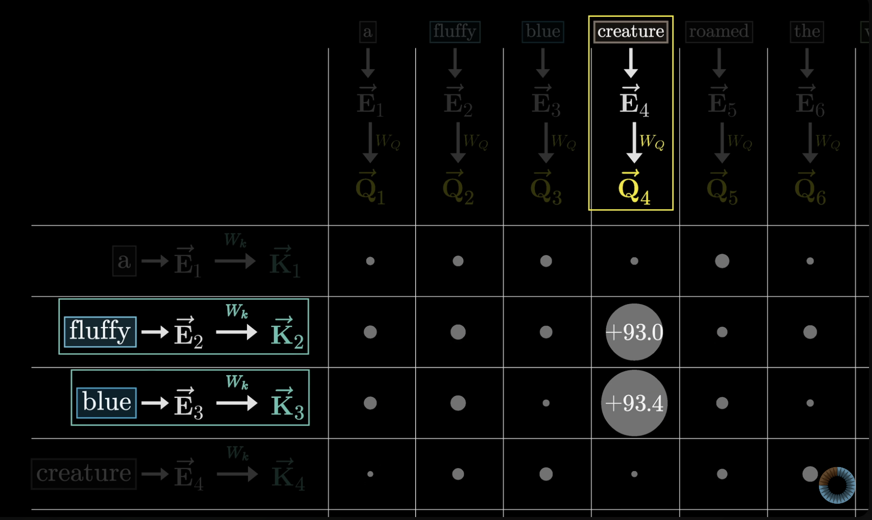
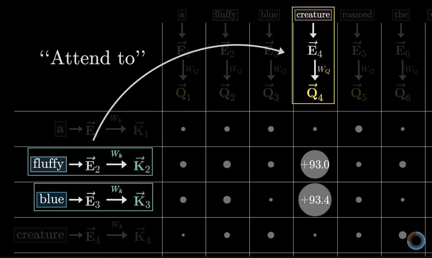

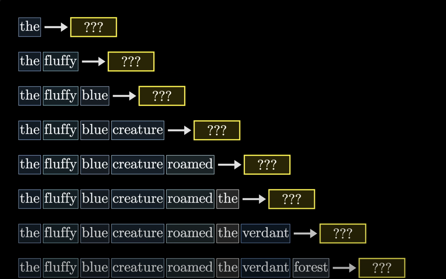
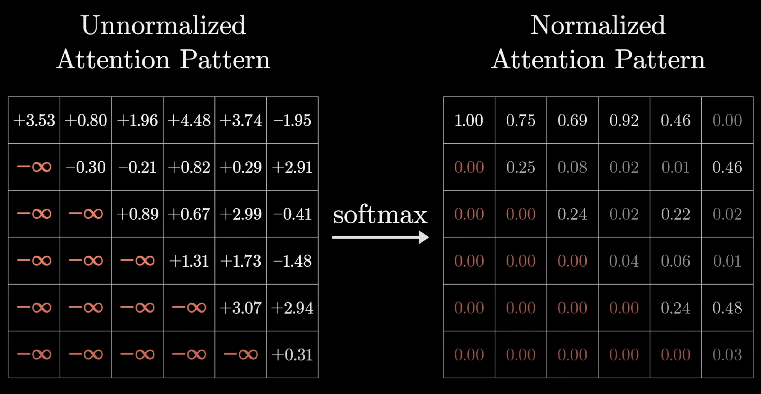
Masking is to prevent later tokens influencing earlier ones during the training process. This is done by setting the entries of the older tokens to -infinity. So when softmax is applied, they are turned to 0.
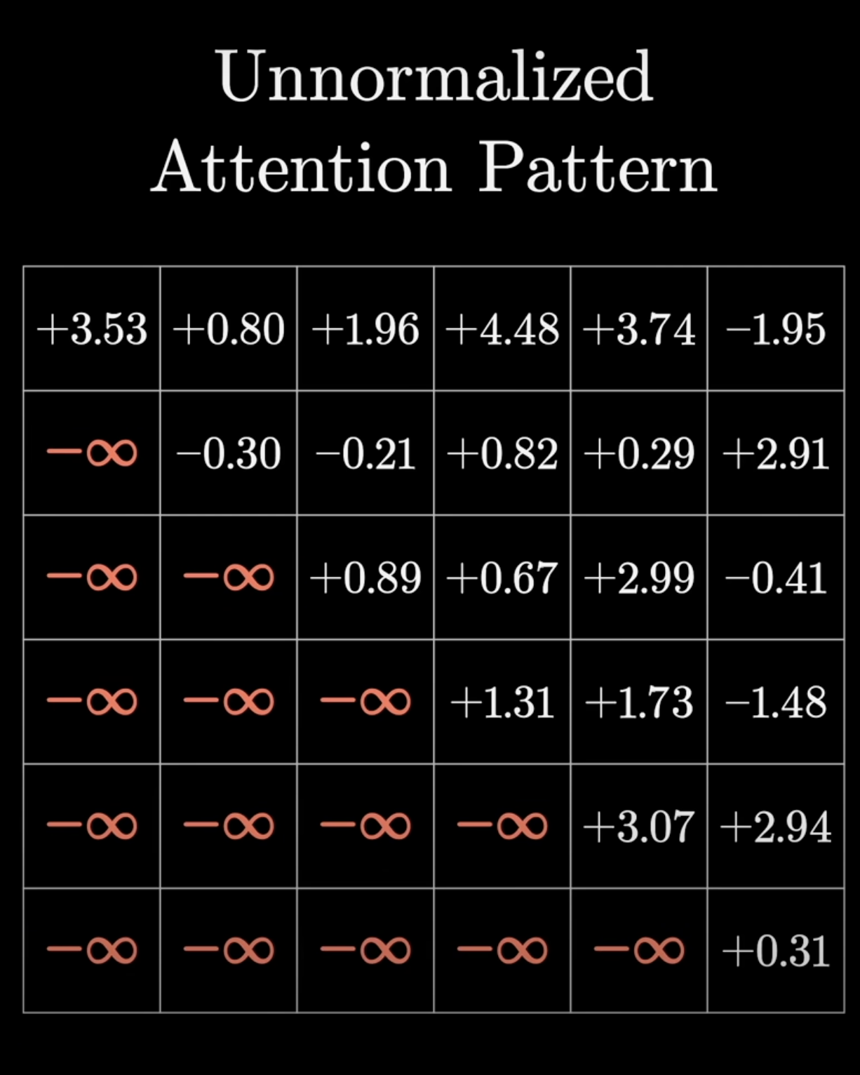
Why mask?
After masking, softmax (normalization) is applied. Masking was done to ensure that later tokens do not affect earlier tokens in the training process. So, the older tokens' entries are set to -infinity during the masking phase, to be transformed into 0 with softmax.
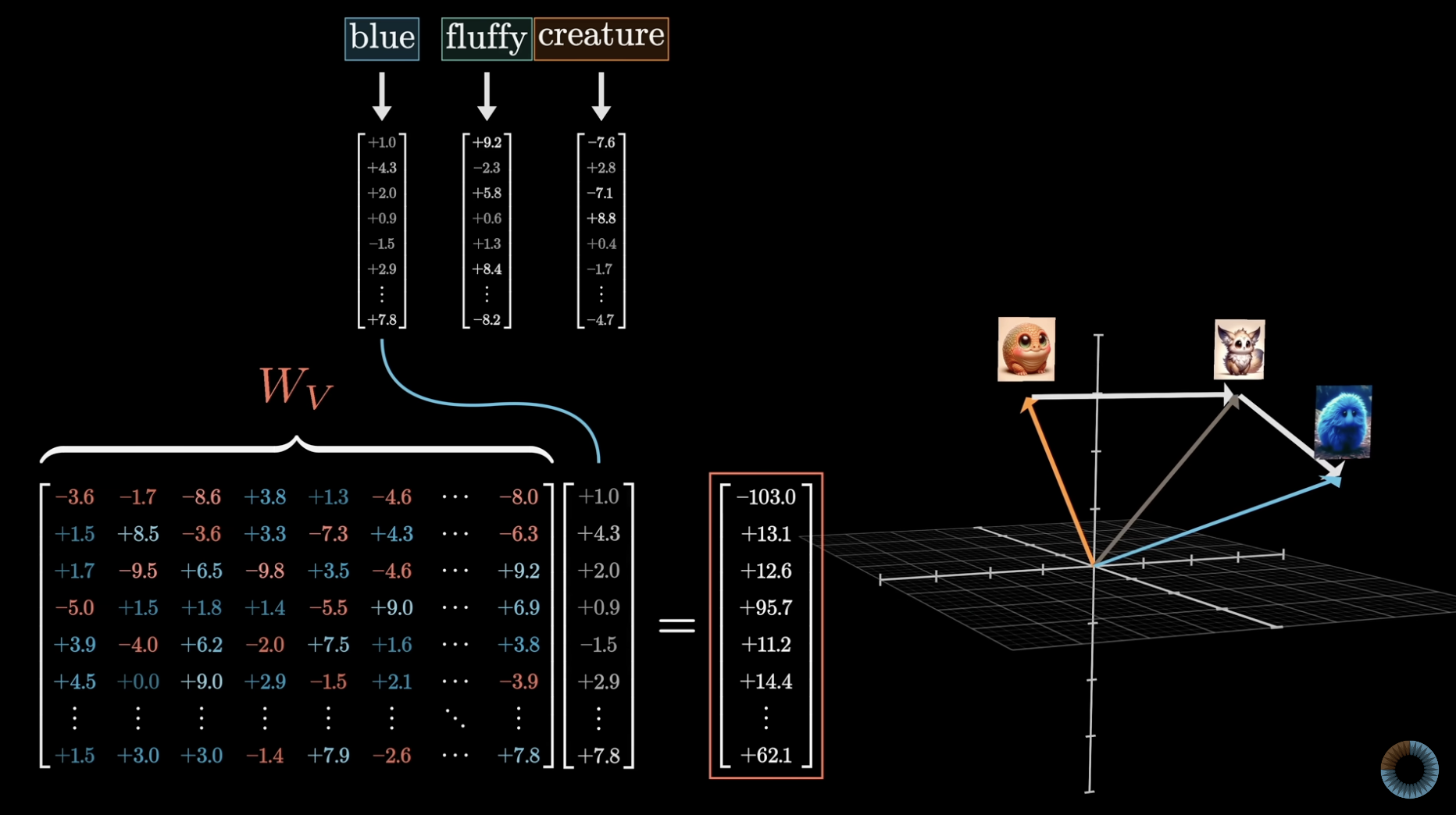
Value matrix W_v is multiplied by the embedding of a word, and this is added to the embedding of the next word
Values essentially answer: IF a word is relevant to adjusting the meaning of something, what exactly should be added to the embedding of that something else, in order to reflect this?
Value: vector that holds the actual info that will be passed along the next layer of the network if a word is deemed relevant based on the attention scores
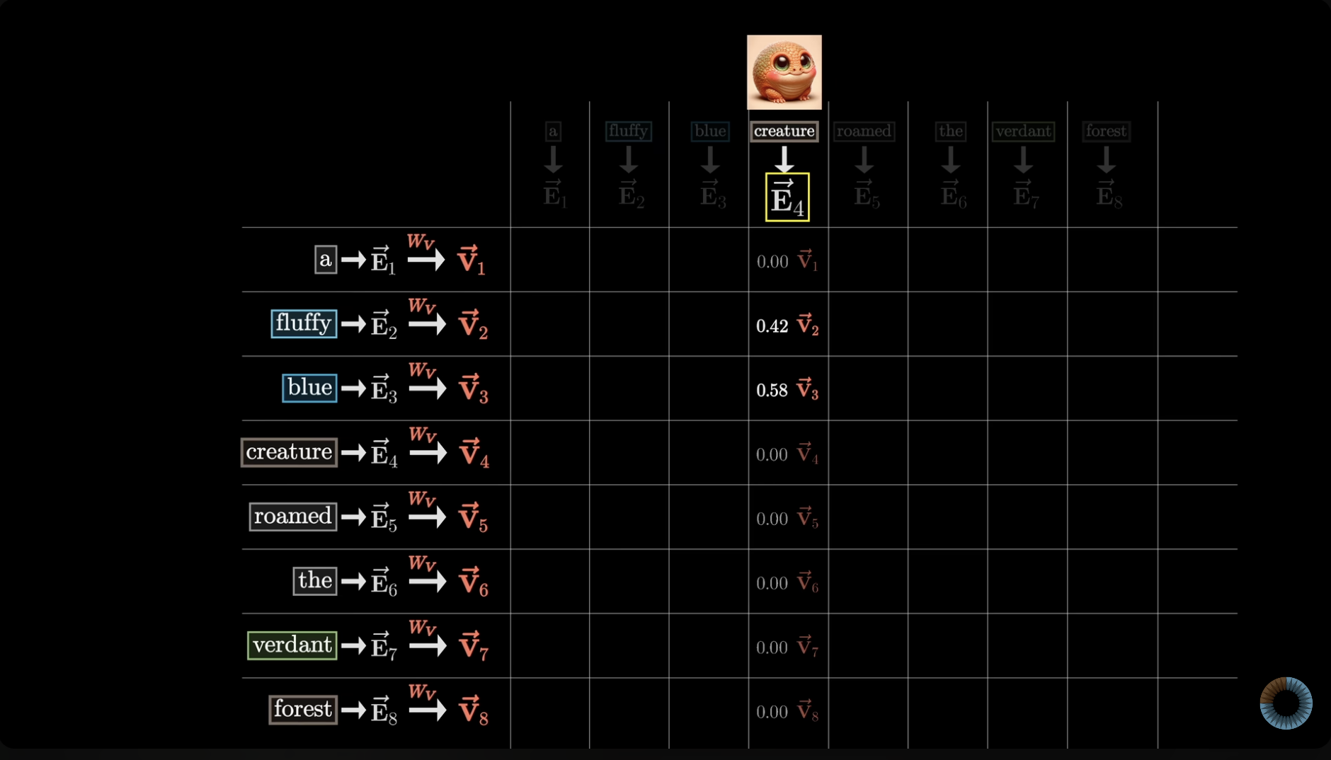
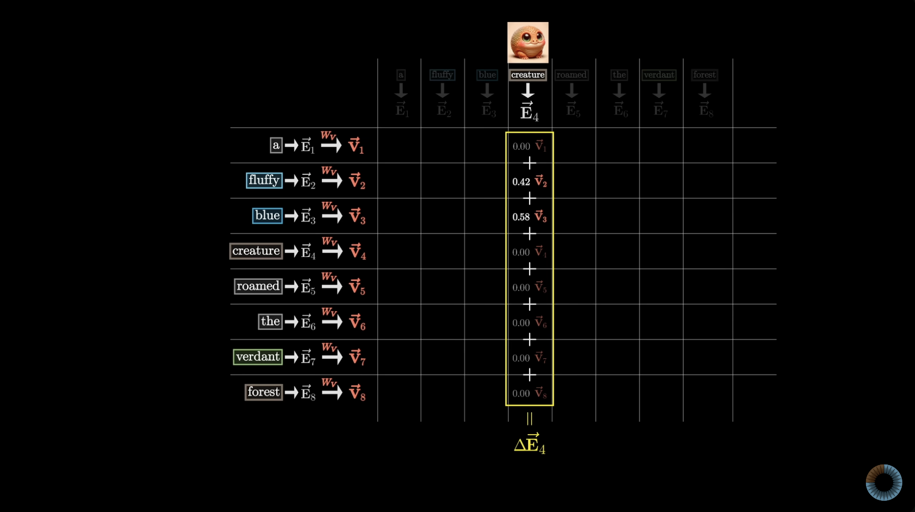
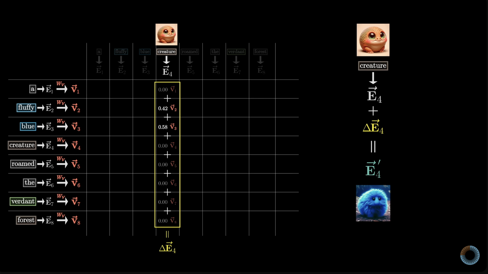
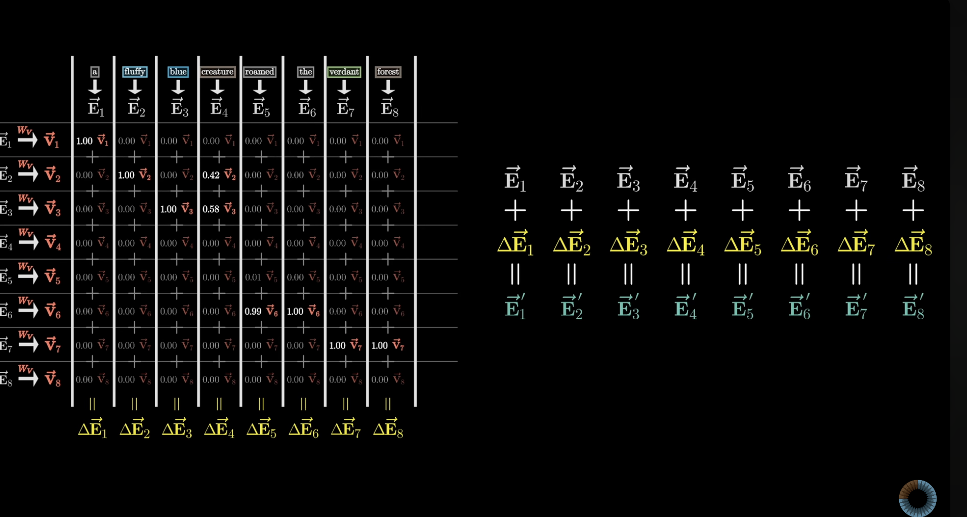
Self-attention is used to update each token’s embedding to include ITS CONTEXT. Each output vector is a contextualized representation of a token, meaning it encodes the original token plus relevant information from all other tokens, so the model can understand the meaning of each token in context, not in isolation.
Self-attention is a sequence-to-sequence operation: a sequence of vectors goes in, and a sequence of vectors comes out.
These are computed as linear projections:
Q = x @ Weights_Q
K = x @ Weights_K
V = x @ Weights_V
Projection: a linear transformation that maps a vector space onto a subspace, such that applying the transformation twice produces the same result as applying it once. It can be visualized as the "shadow" of a vector onto a line or subspace, representing the component of the vector that lies in the direction of that subspace
To determine which other tokens are most relvant to the current token, calculate the similarity between the current token's Q (what its looking for) and every other token's K (what they can offer).
So for each token, we compare its Q to every other token’s K using a dot product:
score[i][j] = dot(Q_i, K_j)
This gives us a matrix of attention scores - raw relevance scores between every token pair.
Then, we apply softmax to each row (i.e., for each token’s scores over the others):
attention_weights = softmax(score)
This turns the raw scores into a probability distribution - i.e., a set of weights that sum to 1, indicating how much each token should pay attention to others (like a percentage). This is handy for the weighted average in the next step.
Recall: A weighted average gives different importance to each value. For example, given values [2, 5, 9] and weights [0.1, 0.3, 0.6], the weighted average is:
(0.1 x 2) + (0.3 x 5) + (0.6 x 9) = 7.1
Now, each token will actually get what it wants from the other tokens.
This is done by taking the weighted sum of the attention weights and the V vectors.
I.e. for token i, compute the weighted sum of all the Value vectors V_j and the attention matrix W_qk (derived from step 2: Q · K and softmax):
output_i = (W_qk[i][0] * V_0) + (W_qk[i][1] * V_1) + (W_qk[i][2] * V_2) + ... + (W_qk[i][n] * V_n)
Or more compactly:
output_i = sum over j of ( W_qk[i][j] * V_j )
Where:
W_qk[i][j] is the attention weight from token i to token jV_j is the Value vector of token joutput_i is the final context-aware embedding for token iThe output is a sequence of vectors, where each vector represents the original tokens WITH ITS CONTEXT (i.e. each vector is a contextualized representation of a token, meaning it encodes the original token plus relevant information from all other tokens.)
The shape of the output is: [sequence_length, hidden_dim]
where:
sequence_length: the number of tokens in the input / length of input sequencehidden_dim: the dimension of the Value vectors (typically same as input embedding dim)| Term | When it’s used | Meaning |
|---|---|---|
| embedding_dim | Input layer | Dimensionality of token embeddings |
| hidden_dim | Inside model (transformer layers) | Dimensionality of internal representations |
Self-attention takes each token, lets it query all other tokens’ keys, figures out how relevant they are, then gathers the most relevant values to build a new, smarter, context-aware embedding of the token.
Below is an implementation of self-attention, from scratch!
from transformers import AutoTokenizer, AutoModel
import torch
from torch import nn


input_text = "Despite everything, it's still you."

# 1. Get input embeddings

# Tokenize input
tokenizer = AutoTokenizer.from_pretrained("bert-base-uncased")
input_tokens = tokenizer(input_text, return_tensors="pt")
print(input_tokens)

# Get raw input embeddings from tokenized input
model = AutoModel.from_pretrained("bert-base-uncased")
outputs = model(**input_tokens)

input_embeddings = outputs.last_hidden_state  # shape: [batch, seq_len, embedding_dim]


# 2. Get Q, K, V

# Initialize projection matrices
hidden_dim = input_embeddings.shape[2]      # dimensionality of full model layer (768)
head_dim = 64                               # dimensionality of each attention head (64 * 12 heads = 768)

W_q = nn.Linear(hidden_dim, head_dim, bias=False)   # input @ W.T
W_k = nn.Linear(hidden_dim, head_dim, bias=False)
W_v = nn.Linear(hidden_dim, head_dim, bias=False)

# Get projections Q, K, V from input
Q = W_q(input_embeddings)
K = W_k(input_embeddings)
V = W_v(input_embeddings)

print(Q.shape)
print(K.shape)

# 3. Get attention scores

# calculate attention scores
K_transposed = K.transpose(-2, -1)      # [batch, seq_len, head_dim] -> [batch, head_dim, seq_len]
attention_scores = torch.matmul(Q, K_transposed)    # Q: [batch, seq_len, head_dim] x K.T: [batch, head_dim, seq_len] -> [batch, seq_len, seq_len]

# apply softmax to normalize attention weights
normalize = nn.Softmax(dim=-1)
attention_weights = normalize(attention_scores / (head_dim ** 0.5))


# 4. Get output

# calculate output vectors: weighted sum of (W_qk) and V vectors
output_tensors = torch.matmul(attention_weights, V)  # shape: [batch, seq_len, head_dim]
print(output_tensors)
An Attention block is made up of many Attention heads running in parallel (multi-headed attention)
By running many distinct heads in parallel, we are giving the model the capacity to learn many distinct ways that context changes meaning
In other words, multiple instances of Self Attention class running in parallel, each instance with different weight matrices
Steps:
The reason for concatenating the outputs from all heads is that each head has learned something different about the input. By concatenating, we combine these insights into a single, unified representation
The final linear transformation is applied to this concatenated output to bring it back to the original embedding dimension
a. Concatenation In multi-head attention, each head learns different aspects of the input because each head operates on a different part of the embedding (head_dim). By concatenating the outputs from all the heads, we are combining these different learned representations into a single vector that encapsulates all these different insights
b. Final linear transformation The final linear transformation, done using a weight matrix, mixes the information from the different heads back into a single vector of the original embedding_dim. This step is crucial because it allows the model to create a unified representation that integrates the different perspectives learned by each head
Credit to 3blue1brown for the visuals!
Deep learning models (like transformers with attention) require compute-heavy operations. One common example is matrix multiplication, which can become extremely resource-intensive when models are large and process lots of data.
To make this faster and more scalable, we can distribute the computation across multiple devices. Each device performs a portion of the work - such as a slice of a large matrix multiplication - in parallel.
Parallelism.
To distribute a workload means to run it in parallel across multiple devices. There are several kinds of parallelism, with the most common being:
Data Parallelism (DP) - parallelism over the data
Tensor Parallelism (TP) - parallelism over the model weights
Sequence Parallelism (SP) - parallelism over the sequence length
In DP, each device gets a copy of the full model, but works on a different shard of the input data.
Let’s say the input tensor is shaped like:
tensor = [batch, height, width, dimension]

Then:
sharded_tensor = [batch / num_devices, height, width, dimension]
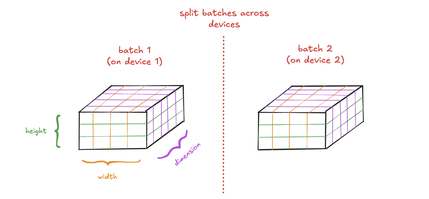
Replicate the model weights across all devices
To emphasize: Effectively, each device contains a replica of the model and is responsible for computing a shard (of the final output tensor).
Run the model on each device - each device uses its replicated model to process its own sharded input data independently
Gather all shards across the devices
Concatenate the shards to form the final output tensor
✅ Use Data Parallelism when model weights fit on a single device, but batch size is large
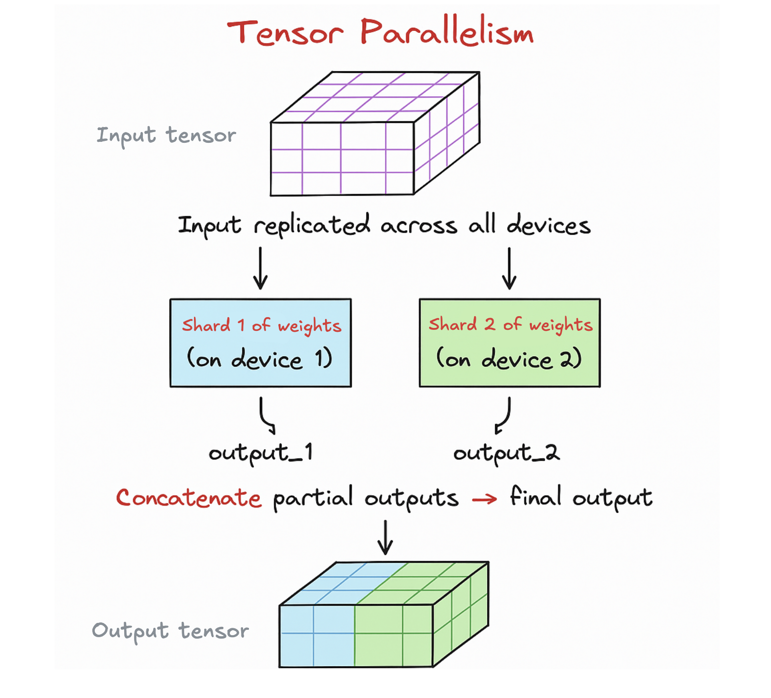
In Tensor Parallelism, the model weights are too large to fit on a single device. So, instead of sharding the data, we shard the model (model parameters/weights) itself.
Steps:
Shard the model parameters across devices
Replicate the input data across all devices (or just the necessary part)
Each device performs computations with its shard of the weights
Gather partial outputs from all devices
Depending on how the weights were sharded:
Continue to the next layer
✅ Use Tensor Parallelism when model weights are too large for a single device.
| Data Parallelism 🧍🧍🧍🧍 | Tensor Parallelism 🧠🔪 | |
|---|---|---|
| What is split? | Input data (batches) | Model weights |
| What is replicated? | Model weights | Input data (or parts of it) |
| Goal | Run the same model on different inputs | Run one input by splitting the model across devices |
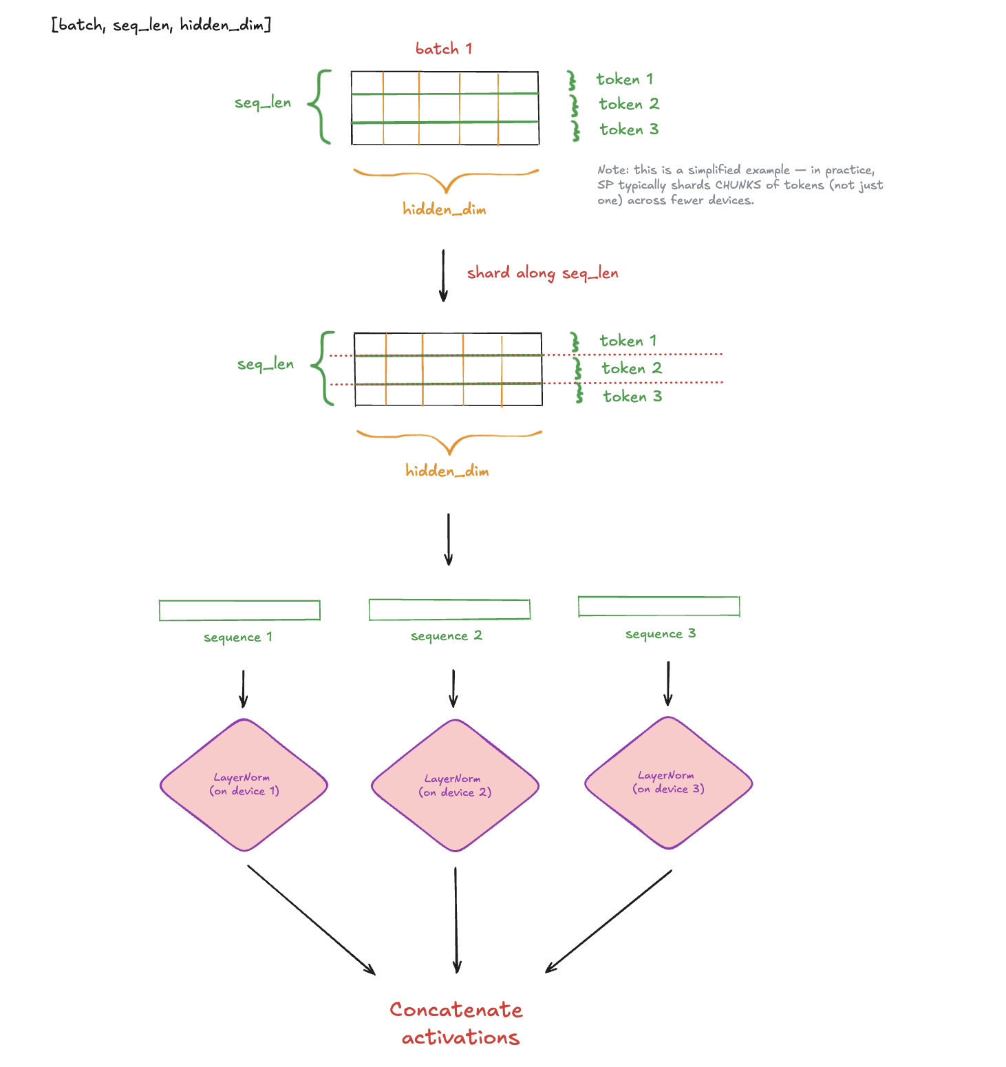
Sequence Parallelism is an extension of Tensor Parallelism. It shards the input along the sequence length - especially helpful for operations like LayerNorm or RMSNorm, which depend on the full sequence.
Why use it? - During training of large models, activation memory (i.e., memory used to store intermediate results like hidden states) becomes a bottleneck - SP reduces activation memory needs by distributing LayerNorm-like computations across devices, in parallel over the sequence
✅ Sequence Parallelism is typically applied only to specific layers like LayerNorm in large-scale TP setups.
When performing Tensor Parallelism, large weight matrices are split across devices so each device only stores and processes a portion. There are two main ways to do this: Column Sharding and Row Sharding.
Assume we have a weight matrix W with shape [input_dim, output_dim].
📌 In column sharding, you split the matrix along the output dimension - i.e., the columns
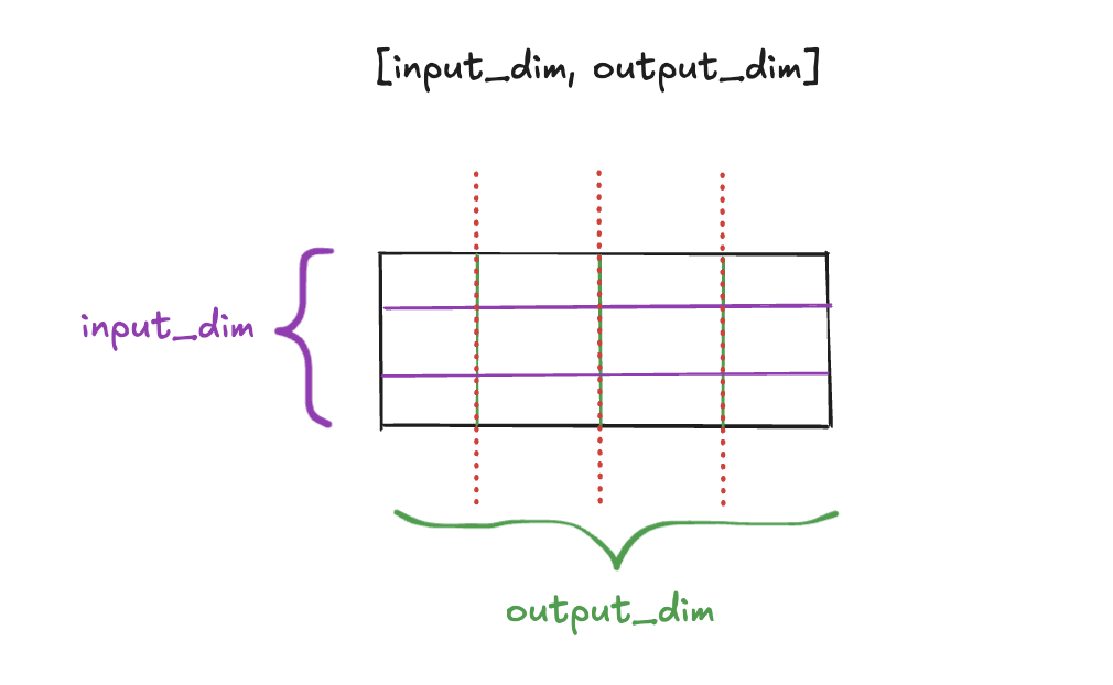
For example, let W = [input_dim, output_dim] = [4, 6]. If we have 2 devices, then:
→ (last dimension is halved/sharded)
Suppose the input is shaped [batch, input_dim]
Each device gets the same input (i.e. input is replicated), and performs matrix multiplication with its own shard of W:
partial_1 = input @ W1 → shape [batch, 3]partial_2 = input @ W2 → shape [batch, 3]These are partial outputs - each covering a subset of the output features.
What do we do next?
The final step is to reconstruct the full output by joining the partial results from each device.
Do this by concatenating along the last dimension:
final_output = torch.cat([partial1, partial2], dim=-1)
This gives you the complete [batch, output_dim] output.
In row sharding, we split the weight matrix W along the input dimension - i.e., the rows.
📌 That means each device holds a subset of the input features that the full matrix would have processed.
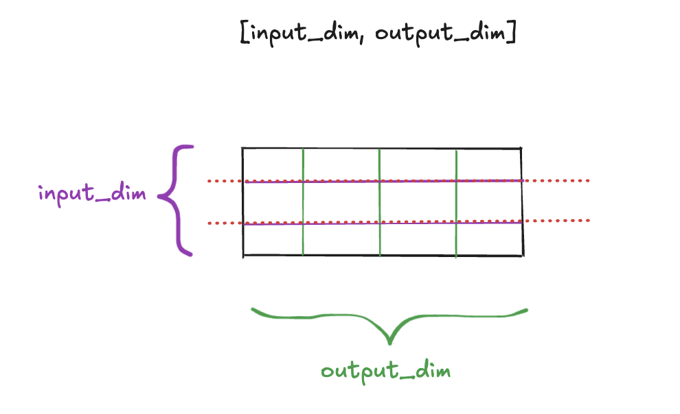
Assume the full weight matrix is W = [4,6]
If we have 2 devices, then:
→ (ie., the first dimension is split evenly across devices)
Follow the same subsequent process as column sharding...
| Sharding Type | How the Weight Matrix is Split | How the Input is Handled | How the Output is Combined | When to Use |
|---|---|---|---|---|
| Column | Split along output dimension | Input is replicated | Concatenate along last dim | When output can be built from feature slices (e.g., MLPs, attention outputs) |
| Row | Split along input dimension | Input is sharded/split | Reduce (e.g., sum) | When each shard contributes to the full output (e.g., QKV projections) |
363 followers · starred Aug 2025
248 followers · starred Aug 2025
55 followers · starred Aug 2024
179 followers · starred Jan 2025
Implementations of ML, using only numpy.
In the context of artificial neural networks:
"weight"The activation of a neuron is calculated based on:
Here's how it works:
"bias"This can be represented by the formula:
weighted_sum = w1*a1 + w2*a2 + ... + wn*an + bias
Where:
w_i is the weight of the connection from neuron i in the previous layera_i is the activation of neuron i in the previous layer
The bias shifts the activation function.
After calculating the weighted sum, we apply an "activation function". Common choices include:
In this guide, we'll focus on ReLU:
def relu(self, x):
        return np.maximum(0, x)
ReLU is popular because it helps the network learn more effectively.
Now that we understand the basic structure and operation of a neural network, let's look at how it learns.
This is the process of passing input through the network to get an output:
To train our network, we need to measure how well it's doing. We do this with a loss function:
The result is called the "loss".
def mse_loss(self, y, activations):
        return np.mean((activations-y)**2)
Thus, we aim to minimize the loss. We do this using:
To improve the network's performance, i.e. minimize the loss, we need to adjust its weights and biases. We do this using two key concepts:
Here's how it works:
Optimization algorithm to minimize the loss function.
Uses gradients to update/adjust weights and biases in the direction that minimizes the loss.
We look for the negative gradient of the loss function, which tells us how we need to change the weights and biases to most efficiently decrease the loss
Backpropagation is the algorithm used to CALCULATE these gradients
The algorithm for determining how a SINGLE training example would like to nudge the weights and biases; not just if they should go up or down, but in terms of what relative proportions to those changes cause the most rapid decrease to the loss.
Activation is influenced in three ways:
w1*a1 + w2*a2 + ... + wn*an + bias
"Propagate backwards": backpropagation is applied in the direction from the last layer to the first layer.
------
∂C/∂w = ∂C/∂a × ∂a/∂z × ∂z/∂w
where C is loss/cost, w is weight, a is activation (output of neuron), z is the weighted sum (input to neuron, before activation).
This tells us how much the loss/cost (error) would change if we slightly adjusted a particular weight.
Averaged nudges to each weight and bias is the negative gradient of the loss function.
Training a neural network involves repeating these steps many times:
After many iterations, the network learns to recognize patterns in the training data and can apply this knowledge to new, unseen data.
For example: in digit recognition, each layer of the neural network can learn to detect common shapes (such as loops, curves, and vertical lines) that act as building blocks for recognizing all digits.
Here's a basic implementation of a neural network (feed-forward, multilayer percepton) from scratch in Python:
Manages multiple layers
Implements forward pass through all layers
Implements the training loop, including:
import numpy as np
import struct
import os
class Neuron:
    def __init__(self, num_inputs):
        self.weights = np.random.randn(num_inputs, 1) * 0.01
        self.bias = np.zeros((1, 1))
        self.last_input = None
        self.last_output = None

    def relu(self, z):
        return np.maximum(0, z)

    def relu_derivative(self, z):
        return np.where(z > 0, 1, 0)

    def forward(self, activations):
        self.last_input = activations
        z = np.dot(activations, self.weights) + self.bias
        self.last_output = self.relu(z)
        return self.last_output

    def backward(self, dC_da, learning_rate):
        da_dz = self.relu_derivative(self.last_output)
        dC_dz = dC_da * da_dz
        dC_dw = np.dot(self.last_input.T, dC_dz)
        dC_db = np.sum(dC_dz, axis=0, keepdims=True)

        self.weights -= learning_rate * dC_dw
        self.bias -= learning_rate * dC_db

        return np.dot(dC_dz, self.weights.T)


    # output_gradient:
        # A positive gradient means we need to decrease that output
        # A negative gradient means we need to increase that output

    # learning_rate: how big of a step is taken while updating weights and biases


class Layer:
    def __init__(self, num_neurons, num_inputs_per_neuron):
        self.neurons = [Neuron(num_inputs_per_neuron) for _ in range(num_neurons)]

    def forward(self, activations):
        return np.hstack([neuron.forward(activations) for neuron in self.neurons])

    def backward(self, output_gradient, learning_rate):
        return np.sum([neuron.backward(output_gradient[:, [i]], learning_rate) for i, neuron in enumerate(self.neurons)], axis=0)

class NeuralNetwork:
    def __init__(self, layer_sizes):
        self.layers = []
        for i in range(len(layer_sizes) - 1):
            self.layers.append(Layer(layer_sizes[i+1], layer_sizes[i]))

    def forward(self, activations):
        for layer in self.layers:
            activations = layer.forward(activations)
        return activations

    def mse_loss(self, y, activations):
        return np.mean((activations-y)**2)

    def derivative_mse_loss(self, y, activations):
        return 2*(activations-y) / y.shape[0]

    def train(self, X, y, epochs, learning_rate, batch_size=32):
        for epoch in range(epochs):
            total_loss = 0
            for i in range(0, len(X), batch_size):
                X_batch = X[i:i+batch_size]
                y_batch = y[i:i+batch_size]

                outputs = self.forward(X_batch)
                loss = self.mse_loss(y_batch, outputs)
                total_loss += loss * len(X_batch)

                output_gradient = self.derivative_mse_loss(y_batch, outputs)
                for layer in reversed(self.layers):
                    output_gradient = layer.backward(output_gradient, learning_rate)

            avg_loss = total_loss / len(X)
            print(f"Epoch {epoch+1}/{epochs}, Loss: {avg_loss}")

    def predict(self, X):
        return self.forward(X)
If you'd like a video format version, see the video below:
A collection of real numbers, which could be:
A probability distribution over all potential next tokens
Tokens are "little pieces" of information (ex. words, combinations of words, sounds, images)
Words that are used and occur in the same context tend to purport similar meanings (distributional semantics)
See Transformer/embedding_notes.ipynb for more on embeddings!
Below is an image of the embedding matrix. Each word corresponds to a specific vector, with no reference to its context. It is the Attention block's responsibility to update a word's vector with its context. (to be discussed later)
Positional encoding provides info about the order of tokens in a sequence.
NOTE: word embeddings & positional embeddings are separate. Word embeddings capture SEMANTIC MEANING, while positional encodings capture the ORDER of tokens
In determining desired output of the transformer (a probability distribution of all possible tokens that can come next in the generating text), a well trained network on the particular dataset is able to determine the next best possible token by:
The desired output of a transformer is a probability distribution of all possible tokens that can come next in the generating text
A probability distribution is defined as a sequence of numbers between 0-1, and that sums to 1. Softmax can give any sequence of numbers these criteria
import numpy as np

# given a sequence of numbers, each term `i`

# softmax eqn:      e^i/(sum of e^i for all terms)

# probability distribution:
    # 1) all numbers are positive numbers 0-1  (e^i)
    # sum of all numbers = 1 (sum of e^i of all terms)

seq = [2, 4, 5]
print(np.exp(seq)/np.sum(np.exp(seq)))
# [0.03511903 0.25949646 0.70538451]
With softmax, the constant T added to the denominator of the exponents of e in the equation can cause more creative generated text
Goal: enable the model to focus on different parts of the input sequence when producing an output for a specific token
A value that represents how much focus (or attention) one word should give to another word in the sequence
(Its derivation is explained later)
Updates a word's embedding vector in reference to its context. Enables the transfer of information from one embedding to another
Prior to Attention, the embedding vector of each word is consistent, regardless of its context (embedding matrix). Therefore, the motivation of Attention is to update a word's embedding vector depending on its context (i.e. surrounding tokens) to capture this specific contextual instance of the word
The computation to predict the next token relies entirely on the final vector of the current sequence
Initially, this vector corresponds to the embedding of the last word in the sequence. As the sequence passes through the model's attention blocks, the final vector is updated to include information from the entire sequence, not just the last word. This updated vector becomes a summary of the whole sequence, encoding all the important information needed to predict the next word
Goal: series of computations to produce a new refined set of embeddings
ex. Have nouns ingest the meanings of their corresponding adjectives
Query: represents the "question"/"focus" that the single-head attention is asking about the current word ex. if the current word is "cat" in the sentence "The cat sat on the mat", the Query for "cat" might be asking, "Which other words (Keys) in this sentence should I focus on to understand cat better?"
Key: serves as a criterion/reference point against which the Query is compared to determine the relevance of each word
Attention Score: tells us how relevant each word is
calculated as: the dot product between the Query and Key vectors
Input: Query, Key and Value matrices
Output: matrix where each vector is the weighted sum of the Value vectors, where the weights come from the attention scores (which are based on the dot product of the Query and Key matrices)
Steps:
The higher the dot product, the more relevant the Query to the Key (i.e. word to another word in the sentence)
Masking is to prevent later tokens influencing earlier ones during the training process. This is done by setting the entries of the older tokens to -infinity. So when softmax is applied, they are turned to 0.
Why mask?
After masking, softmax (normalization) is applied. Masking was done to ensure that later tokens do not affect earlier tokens in the training process. So, the older tokens' entries are set to -infinity during the masking phase, to be transformed into 0 with softmax.
Value matrix W_v is multiplied by the embedding of a word, and this is added to the embedding of the next word
Values essentially answer: IF a word is relevant to adjusting the meaning of something, what exactly should be added to the embedding of that something else, in order to reflect this?
Value: vector that holds the actual info that will be passed along the next layer of the network if a word is deemed relevant based on the attention scores
Self-attention is used to update each token’s embedding to include ITS CONTEXT. Each output vector is a contextualized representation of a token, meaning it encodes the original token plus relevant information from all other tokens, so the model can understand the meaning of each token in context, not in isolation.
Self-attention is a sequence-to-sequence operation: a sequence of vectors goes in, and a sequence of vectors comes out.
These are computed as linear projections:
Q = x @ Weights_Q
K = x @ Weights_K
V = x @ Weights_V
Projection: a linear transformation that maps a vector space onto a subspace, such that applying the transformation twice produces the same result as applying it once. It can be visualized as the "shadow" of a vector onto a line or subspace, representing the component of the vector that lies in the direction of that subspace
To determine which other tokens are most relvant to the current token, calculate the similarity between the current token's Q (what its looking for) and every other token's K (what they can offer).
So for each token, we compare its Q to every other token’s K using a dot product:
score[i][j] = dot(Q_i, K_j)
This gives us a matrix of attention scores - raw relevance scores between every token pair.
Then, we apply softmax to each row (i.e., for each token’s scores over the others):
attention_weights = softmax(score)
This turns the raw scores into a probability distribution - i.e., a set of weights that sum to 1, indicating how much each token should pay attention to others (like a percentage). This is handy for the weighted average in the next step.
Recall: A weighted average gives different importance to each value. For example, given values [2, 5, 9] and weights [0.1, 0.3, 0.6], the weighted average is:
(0.1 x 2) + (0.3 x 5) + (0.6 x 9) = 7.1
Now, each token will actually get what it wants from the other tokens.
This is done by taking the weighted sum of the attention weights and the V vectors.
I.e. for token i, compute the weighted sum of all the Value vectors V_j and the attention matrix W_qk (derived from step 2: Q · K and softmax):
output_i = (W_qk[i][0] * V_0) + (W_qk[i][1] * V_1) + (W_qk[i][2] * V_2) + ... + (W_qk[i][n] * V_n)
Or more compactly:
output_i = sum over j of ( W_qk[i][j] * V_j )
Where:
W_qk[i][j] is the attention weight from token i to token jV_j is the Value vector of token joutput_i is the final context-aware embedding for token iThe output is a sequence of vectors, where each vector represents the original tokens WITH ITS CONTEXT (i.e. each vector is a contextualized representation of a token, meaning it encodes the original token plus relevant information from all other tokens.)
The shape of the output is: [sequence_length, hidden_dim]
where:
sequence_length: the number of tokens in the input / length of input sequencehidden_dim: the dimension of the Value vectors (typically same as input embedding dim)| Term | When it’s used | Meaning |
|---|---|---|
| embedding_dim | Input layer | Dimensionality of token embeddings |
| hidden_dim | Inside model (transformer layers) | Dimensionality of internal representations |
Self-attention takes each token, lets it query all other tokens’ keys, figures out how relevant they are, then gathers the most relevant values to build a new, smarter, context-aware embedding of the token.
Below is an implementation of self-attention, from scratch!
from transformers import AutoTokenizer, AutoModel
import torch
from torch import nn


input_text = "Despite everything, it's still you."

# 1. Get input embeddings

# Tokenize input
tokenizer = AutoTokenizer.from_pretrained("bert-base-uncased")
input_tokens = tokenizer(input_text, return_tensors="pt")
print(input_tokens)

# Get raw input embeddings from tokenized input
model = AutoModel.from_pretrained("bert-base-uncased")
outputs = model(**input_tokens)

input_embeddings = outputs.last_hidden_state  # shape: [batch, seq_len, embedding_dim]


# 2. Get Q, K, V

# Initialize projection matrices
hidden_dim = input_embeddings.shape[2]      # dimensionality of full model layer (768)
head_dim = 64                               # dimensionality of each attention head (64 * 12 heads = 768)

W_q = nn.Linear(hidden_dim, head_dim, bias=False)   # input @ W.T
W_k = nn.Linear(hidden_dim, head_dim, bias=False)
W_v = nn.Linear(hidden_dim, head_dim, bias=False)

# Get projections Q, K, V from input
Q = W_q(input_embeddings)
K = W_k(input_embeddings)
V = W_v(input_embeddings)

print(Q.shape)
print(K.shape)

# 3. Get attention scores

# calculate attention scores
K_transposed = K.transpose(-2, -1)      # [batch, seq_len, head_dim] -> [batch, head_dim, seq_len]
attention_scores = torch.matmul(Q, K_transposed)    # Q: [batch, seq_len, head_dim] x K.T: [batch, head_dim, seq_len] -> [batch, seq_len, seq_len]

# apply softmax to normalize attention weights
normalize = nn.Softmax(dim=-1)
attention_weights = normalize(attention_scores / (head_dim ** 0.5))


# 4. Get output

# calculate output vectors: weighted sum of (W_qk) and V vectors
output_tensors = torch.matmul(attention_weights, V)  # shape: [batch, seq_len, head_dim]
print(output_tensors)
An Attention block is made up of many Attention heads running in parallel (multi-headed attention)
By running many distinct heads in parallel, we are giving the model the capacity to learn many distinct ways that context changes meaning
In other words, multiple instances of Self Attention class running in parallel, each instance with different weight matrices
Steps:
The reason for concatenating the outputs from all heads is that each head has learned something different about the input. By concatenating, we combine these insights into a single, unified representation
The final linear transformation is applied to this concatenated output to bring it back to the original embedding dimension
a. Concatenation In multi-head attention, each head learns different aspects of the input because each head operates on a different part of the embedding (head_dim). By concatenating the outputs from all the heads, we are combining these different learned representations into a single vector that encapsulates all these different insights
b. Final linear transformation The final linear transformation, done using a weight matrix, mixes the information from the different heads back into a single vector of the original embedding_dim. This step is crucial because it allows the model to create a unified representation that integrates the different perspectives learned by each head
Credit to 3blue1brown for the visuals!
Deep learning models (like transformers with attention) require compute-heavy operations. One common example is matrix multiplication, which can become extremely resource-intensive when models are large and process lots of data.
To make this faster and more scalable, we can distribute the computation across multiple devices. Each device performs a portion of the work - such as a slice of a large matrix multiplication - in parallel.
Parallelism.
To distribute a workload means to run it in parallel across multiple devices. There are several kinds of parallelism, with the most common being:
Data Parallelism (DP) - parallelism over the data
Tensor Parallelism (TP) - parallelism over the model weights
Sequence Parallelism (SP) - parallelism over the sequence length
In DP, each device gets a copy of the full model, but works on a different shard of the input data.
Let’s say the input tensor is shaped like:
tensor = [batch, height, width, dimension]
Then:
sharded_tensor = [batch / num_devices, height, width, dimension]
Replicate the model weights across all devices
To emphasize: Effectively, each device contains a replica of the model and is responsible for computing a shard (of the final output tensor).
Run the model on each device - each device uses its replicated model to process its own sharded input data independently
Gather all shards across the devices
Concatenate the shards to form the final output tensor
✅ Use Data Parallelism when model weights fit on a single device, but batch size is large
In Tensor Parallelism, the model weights are too large to fit on a single device. So, instead of sharding the data, we shard the model (model parameters/weights) itself.
Steps:
Shard the model parameters across devices
Replicate the input data across all devices (or just the necessary part)
Each device performs computations with its shard of the weights
Gather partial outputs from all devices
Depending on how the weights were sharded:
Continue to the next layer
✅ Use Tensor Parallelism when model weights are too large for a single device.
| Data Parallelism 🧍🧍🧍🧍 | Tensor Parallelism 🧠🔪 | |
|---|---|---|
| What is split? | Input data (batches) | Model weights |
| What is replicated? | Model weights | Input data (or parts of it) |
| Goal | Run the same model on different inputs | Run one input by splitting the model across devices |
Sequence Parallelism is an extension of Tensor Parallelism. It shards the input along the sequence length - especially helpful for operations like LayerNorm or RMSNorm, which depend on the full sequence.
Why use it? - During training of large models, activation memory (i.e., memory used to store intermediate results like hidden states) becomes a bottleneck - SP reduces activation memory needs by distributing LayerNorm-like computations across devices, in parallel over the sequence
✅ Sequence Parallelism is typically applied only to specific layers like LayerNorm in large-scale TP setups.
When performing Tensor Parallelism, large weight matrices are split across devices so each device only stores and processes a portion. There are two main ways to do this: Column Sharding and Row Sharding.
Assume we have a weight matrix W with shape [input_dim, output_dim].
📌 In column sharding, you split the matrix along the output dimension - i.e., the columns
For example, let W = [input_dim, output_dim] = [4, 6]. If we have 2 devices, then:
→ (last dimension is halved/sharded)
Suppose the input is shaped [batch, input_dim]
Each device gets the same input (i.e. input is replicated), and performs matrix multiplication with its own shard of W:
partial_1 = input @ W1 → shape [batch, 3]partial_2 = input @ W2 → shape [batch, 3]These are partial outputs - each covering a subset of the output features.
What do we do next?
The final step is to reconstruct the full output by joining the partial results from each device.
Do this by concatenating along the last dimension:
final_output = torch.cat([partial1, partial2], dim=-1)
This gives you the complete [batch, output_dim] output.
In row sharding, we split the weight matrix W along the input dimension - i.e., the rows.
📌 That means each device holds a subset of the input features that the full matrix would have processed.
Assume the full weight matrix is W = [4,6]
If we have 2 devices, then:
→ (ie., the first dimension is split evenly across devices)
Follow the same subsequent process as column sharding...
| Sharding Type | How the Weight Matrix is Split | How the Input is Handled | How the Output is Combined | When to Use |
|---|---|---|---|---|
| Column | Split along output dimension | Input is replicated | Concatenate along last dim | When output can be built from feature slices (e.g., MLPs, attention outputs) |
| Row | Split along input dimension | Input is sharded/split | Reduce (e.g., sum) | When each shard contributes to the full output (e.g., QKV projections) |
363 followers · starred Aug 2025
248 followers · starred Aug 2025
55 followers · starred Aug 2024
179 followers · starred Jan 2025