Mol-JEPA multimodal molecular foundation model
Jupyter Notebook
28
0 commits
updated Oct 14, 2026
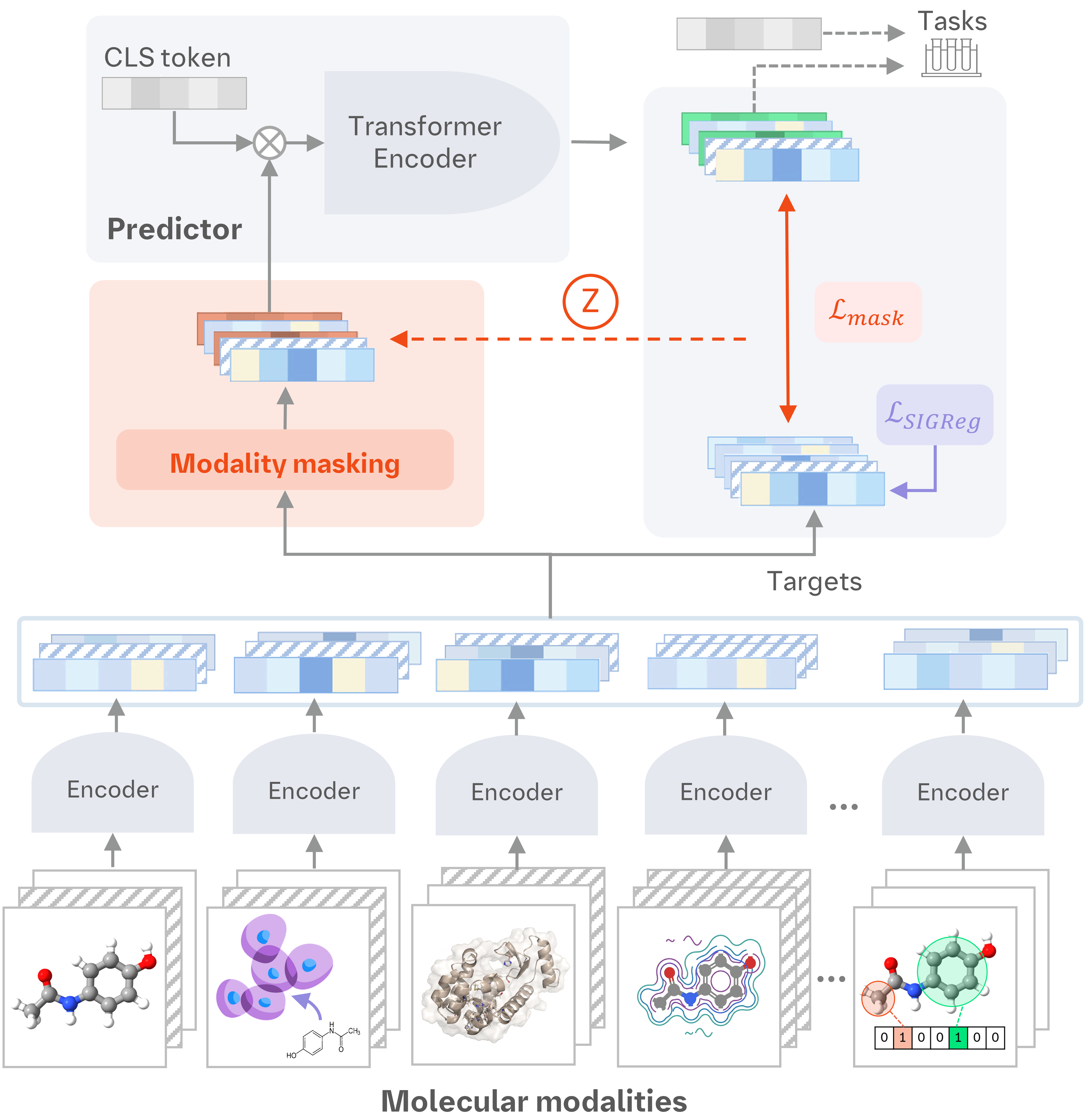
This is the code for Mol-JEPA, a scalable framework for learning molecular world models from diverse physical and biochemical modalities that go beyond the molecular structure. Using a novel multi-modal joint embedding predictive architecture, we efficiently fuse information from various pretrained models and datasets, including cellular effects, binding affinity, ADMET properties and quantum chemistry. Across relevant benchmarks, we show that the representations learned by Mol-JEPA achieve competitive performance, marking an important step towards more comprehensive molecular foundation models.
The easiest way to use Mol-JEPA is through Huggingface, which provides the model checkpoint with an inference module for batching. First install the required libraries:
pip install torch torch-geometric transformers safetensors rdkit molfeat numpy
Then you can generate embedding vectors as follows. Mol-JEPA provides three outputs: the CLS token as global summary, per-modality predicted embeddings and per-modality latent embeddings before the readout layer. The inference module expects a list of smiles, which will be processed as a batch.
from transformers import AutoModel

model = AutoModel.from_pretrained("Flogrammer/Mol-JEPA", trust_remote_code=True)
model.eval()

smiles_list = ["Cn1cnc2n(C)c(=O)n(C)c(=O)c12", "CC(=O)Oc1ccccc1C(=O)O"]
out = model(smiles_list)

print("Predicted embeddings shape:", out.predictions.shape) # batch size, modalities, embedding dimension
>>> Predicted embeddings shape: torch.Size([2, 12, 512])

print("CLS token shape:", out.cls.shape) # batch size, embedding dimension
>>> CLS token shape: torch.Size([2, 512])

print("Latent embeddings shape:", out.embeddings.shape) # batch size, modalities (+ CLS), latent dimension
>>> Latent embeddings shape: torch.Size([2, 13, 512])
Note that while TabICL + CLS tokens is the quickest way, it might not always lead to the best performance. We encourage to experiment with other embeddings and probe models, as we experienced quite some variance in performance across datasets.
The multimodal dataset is available on huggingface and can be loaded as described below. In contains a metadata table that links SMILES / InChi codes to the modalities, which are stored in numpy arrays. Note that the full dataset has a size of 313 GB when unzipped.
from datasets import load_dataset

metadata = load_dataset("Flogrammer/Mol-JEPA-dataset")
metadata.head()
You can also train your own model and add additional modalities. The overall training logic is based on the stable-pretraining library and config files control most of the important properties. The config used by the Huggingface model can be found here: src/config/moljepa.yaml.
Install the requirements.txt for model training and then simply launch the training by
train.py --config-name=moljepa
For more advanced options see the train.bash script which parallelizes training on multiple GPUs using SLURM.
Our framework allows to easily add additional modalities. The base class is defined in src/models/backbones/base.py and specifies the required functions for a new modality module. In the same directory you can find several examples for modality definitions. On one hand, we support different backbone types:
and secondly, they can be:
The metadata table name serves as a unique identifier and all processed modalities will be stored as tensors on the disk, to avoid re-processing them on every training launch. The code will automatically check if new modalities were added and only processes those.
To use new modalities, simply add them to the modalities field in the config file. For this you need to specify a few properties, for example if the modality has been pre-computed or its dimensionality. All samples are stored as tensor files on disk once processed. Also make sure a path-column in the metadata table exists.
# Example 1
- name: uma # Modality name
  input: precomputed_node # Atom-level precomputed
  output: atoms # the output shape. atoms means [n_atoms, n_features]
  colname: uma_embedding_path # The column name in the metadata table
  node_dim: 128 # dimensionality of the node features
  processing: multiprocess # batch size = 1 but multiple workers

# Example 2
- name: ecfp # Modality name
  input: smiles # Here the backbone module expectes a smiles string as input
  output: embedding # shape [1, dim]
  dim: 2048 # embedding dimension
  processing: batch # the module allows batch processing
  batch_size: 64 # Batch size for processing
At the moment, Mol-JEPA only supports static modalities, i.e. we have no option to include learnable encoders.
During training, several callbacks from stable-pretraining are used to monitor the training. For example, different online probes can be defined in the yaml file, which will be displayed on tensorboard during training. Stable-pretraining uses separate optimizer loops for those. More useful callbacks are available in src/callbacks, for example Early Stopping, Gradient tracing, UMAP visualizations and more.
We also provide an example yaml and bash script to perform parallel bayesian hyperparameter tuning using SLURM and Optuna, which can be found at config/moljepa_hp.yaml. The hyperparameter search will automatically log all important information to tensorboard and allows to quickly compare different configurations.
For attention analysis, you can capture and optionally return the Transformer self-attention maps during inference. For this, simply pass return_attn=False in the model forward pass (also works for the Huggingface model) and it will return one tensor per layer with shape [batch, heads, n_modalities, n_modalities].
Our plots and results can be generated using the following notebooks. Below you find a brief summary of each notebook's content.
To run the notebooks, you also need to set several environment variables, such as:
export PROCESSED_DIR="/path/to/processed/data"
export BENCHMARKS_DIR="/path/to/benchmark/results"
export CHECKPOINT_DIR="/path/to/checkpoint/files"
export LOGS_DIR="/path/to/tensorboard/logs"
export CLUSTER_SPLITS_DIR="/path/to/split/files"
If you use MOL-JEPA in your research, please cite:
@misc{rottach2026moljepamultimodaljointembedding,
      title={Mol-JEPA: A multimodal Joint Embedding Predictive Architecture for Molecules},
      author={Florian Rottach and Sebastian Schieferdecker and William Rudman and Randall Balestriero and Carsten Eickhoff},
      year={2026},
      eprint={2608.22642},
      archivePrefix={arXiv},
      primaryClass={cs.LG},
      url={https://arxiv.org/abs/2608.22642},
}
This repository, including the model, source code, documentation, and associated materials, is licensed under the Creative Commons Attribution-NonCommercial 4.0 International (CC BY-NC 4.0) License.
You are free to share, copy, redistribute, adapt, and modify this work for non-commercial purposes, provided that appropriate credit is given to the original author(s), a link to the license is included, and any changes made are clearly indicated.
Commercial use is not permitted without prior written permission from the author(s).
For the full license text, see: https://creativecommons.org/licenses/by-nc/4.0/
Mol-JEPA multimodal molecular foundation model
Jupyter Notebook
28
0 commits
updated Oct 14, 2026
This is the code for Mol-JEPA, a scalable framework for learning molecular world models from diverse physical and biochemical modalities that go beyond the molecular structure. Using a novel multi-modal joint embedding predictive architecture, we efficiently fuse information from various pretrained models and datasets, including cellular effects, binding affinity, ADMET properties and quantum chemistry. Across relevant benchmarks, we show that the representations learned by Mol-JEPA achieve competitive performance, marking an important step towards more comprehensive molecular foundation models.
The easiest way to use Mol-JEPA is through Huggingface, which provides the model checkpoint with an inference module for batching. First install the required libraries:
pip install torch torch-geometric transformers safetensors rdkit molfeat numpy
Then you can generate embedding vectors as follows. Mol-JEPA provides three outputs: the CLS token as global summary, per-modality predicted embeddings and per-modality latent embeddings before the readout layer. The inference module expects a list of smiles, which will be processed as a batch.
from transformers import AutoModel

model = AutoModel.from_pretrained("Flogrammer/Mol-JEPA", trust_remote_code=True)
model.eval()

smiles_list = ["Cn1cnc2n(C)c(=O)n(C)c(=O)c12", "CC(=O)Oc1ccccc1C(=O)O"]
out = model(smiles_list)

print("Predicted embeddings shape:", out.predictions.shape) # batch size, modalities, embedding dimension
>>> Predicted embeddings shape: torch.Size([2, 12, 512])

print("CLS token shape:", out.cls.shape) # batch size, embedding dimension
>>> CLS token shape: torch.Size([2, 512])

print("Latent embeddings shape:", out.embeddings.shape) # batch size, modalities (+ CLS), latent dimension
>>> Latent embeddings shape: torch.Size([2, 13, 512])
Note that while TabICL + CLS tokens is the quickest way, it might not always lead to the best performance. We encourage to experiment with other embeddings and probe models, as we experienced quite some variance in performance across datasets.
The multimodal dataset is available on huggingface and can be loaded as described below. In contains a metadata table that links SMILES / InChi codes to the modalities, which are stored in numpy arrays. Note that the full dataset has a size of 313 GB when unzipped.
from datasets import load_dataset

metadata = load_dataset("Flogrammer/Mol-JEPA-dataset")
metadata.head()
You can also train your own model and add additional modalities. The overall training logic is based on the stable-pretraining library and config files control most of the important properties. The config used by the Huggingface model can be found here: src/config/moljepa.yaml.
Install the requirements.txt for model training and then simply launch the training by
train.py --config-name=moljepa
For more advanced options see the train.bash script which parallelizes training on multiple GPUs using SLURM.
Our framework allows to easily add additional modalities. The base class is defined in src/models/backbones/base.py and specifies the required functions for a new modality module. In the same directory you can find several examples for modality definitions. On one hand, we support different backbone types:
and secondly, they can be:
The metadata table name serves as a unique identifier and all processed modalities will be stored as tensors on the disk, to avoid re-processing them on every training launch. The code will automatically check if new modalities were added and only processes those.
To use new modalities, simply add them to the modalities field in the config file. For this you need to specify a few properties, for example if the modality has been pre-computed or its dimensionality. All samples are stored as tensor files on disk once processed. Also make sure a path-column in the metadata table exists.
# Example 1
- name: uma # Modality name
  input: precomputed_node # Atom-level precomputed
  output: atoms # the output shape. atoms means [n_atoms, n_features]
  colname: uma_embedding_path # The column name in the metadata table
  node_dim: 128 # dimensionality of the node features
  processing: multiprocess # batch size = 1 but multiple workers

# Example 2
- name: ecfp # Modality name
  input: smiles # Here the backbone module expectes a smiles string as input
  output: embedding # shape [1, dim]
  dim: 2048 # embedding dimension
  processing: batch # the module allows batch processing
  batch_size: 64 # Batch size for processing
At the moment, Mol-JEPA only supports static modalities, i.e. we have no option to include learnable encoders.
During training, several callbacks from stable-pretraining are used to monitor the training. For example, different online probes can be defined in the yaml file, which will be displayed on tensorboard during training. Stable-pretraining uses separate optimizer loops for those. More useful callbacks are available in src/callbacks, for example Early Stopping, Gradient tracing, UMAP visualizations and more.
We also provide an example yaml and bash script to perform parallel bayesian hyperparameter tuning using SLURM and Optuna, which can be found at config/moljepa_hp.yaml. The hyperparameter search will automatically log all important information to tensorboard and allows to quickly compare different configurations.
For attention analysis, you can capture and optionally return the Transformer self-attention maps during inference. For this, simply pass return_attn=False in the model forward pass (also works for the Huggingface model) and it will return one tensor per layer with shape [batch, heads, n_modalities, n_modalities].
Our plots and results can be generated using the following notebooks. Below you find a brief summary of each notebook's content.
To run the notebooks, you also need to set several environment variables, such as:
export PROCESSED_DIR="/path/to/processed/data"
export BENCHMARKS_DIR="/path/to/benchmark/results"
export CHECKPOINT_DIR="/path/to/checkpoint/files"
export LOGS_DIR="/path/to/tensorboard/logs"
export CLUSTER_SPLITS_DIR="/path/to/split/files"
If you use MOL-JEPA in your research, please cite:
@misc{rottach2026moljepamultimodaljointembedding,
      title={Mol-JEPA: A multimodal Joint Embedding Predictive Architecture for Molecules},
      author={Florian Rottach and Sebastian Schieferdecker and William Rudman and Randall Balestriero and Carsten Eickhoff},
      year={2026},
      eprint={2608.22642},
      archivePrefix={arXiv},
      primaryClass={cs.LG},
      url={https://arxiv.org/abs/2608.22642},
}
This repository, including the model, source code, documentation, and associated materials, is licensed under the Creative Commons Attribution-NonCommercial 4.0 International (CC BY-NC 4.0) License.
You are free to share, copy, redistribute, adapt, and modify this work for non-commercial purposes, provided that appropriate credit is given to the original author(s), a link to the license is included, and any changes made are clearly indicated.
Commercial use is not permitted without prior written permission from the author(s).
For the full license text, see: https://creativecommons.org/licenses/by-nc/4.0/