Fine-tuning HyenaDNA on a promoter-vs-non-promoter classification task, evaluated against a simple k-mer baseline and interpreted with in-silico mutagenesis and a position-wise classification head readout.
Binary classification: is a 251bp human DNA sequence a non-TATA promoter, or a non-promoter fragment from a gene body?
Dataset: katarinagresova/Genomic_Benchmarks_human_nontata_promoters, part of the GenomicBenchmarks suite. Positive sequences span -200bp to +50bp around a transcription start site (TSS) lacking a TATA box; negatives are random 251bp fragments from human gene regions after the first exon. 36,131 sequences total, 54.4% positive.
Before trusting any result here, the train/test split was audited for the kind of batch effect that produces a suspicious, too-good-to-be-true accuracy. The official GenomicBenchmarks split for this dataset is a plain row-level sklearn.train_test_split(random_state=42) with no chromosome or locus grouping, confirmed directly from the dataset's construction notebook.
A k-mer overlap audit (scripts/check_leakage.py, scripts/check_leakage2.py) found:
scripts/build_clean_split.py rebuilds the split: sequences are clustered by shared 50-mers via union-find (any 50bp exact match implies overlapping loci), then whole clusters are assigned to train or test so no overlapping window crosses the split. scripts/verify_clean_split.py confirms 0% exact and 0% near-duplicate overlap on the result.
Clean split: 26,648 train / 9,483 test, 54.4% positive in both. Saved to data/human_nontata_promoters_clean/. All results below use this split, not the official one. Because of that, numbers here are not directly comparable to published GenomicBenchmarks leaderboard results on this dataset, and are expected to be somewhat lower, since the leaked split likely inflates reported accuracy.
The fine-tuning notebook rebuilds this same clean split from scratch at runtime (same algorithm, same seed), so it doesn't depend on the CSVs in data/ to reproduce.
LongSafari/hyenadna-tiny-1k-seqlen-hf: a 2-layer Hyena (implicit long-convolution) model, d_model=128, 436,352 total parameters, single-character tokenizer (4 nucleotides plus special tokens), max_seq_len=1026. Chosen for its small size and turnkey HuggingFace Trainer integration, making it realistic to fine-tune on free-tier compute.
Loading it requires trust_remote_code=True, which executes custom modeling/tokenizer code from the LongSafari HF repo rather than only transformers-native code. LongSafari is the paper authors' official org, but this is a different trust boundary than a fully first-party checkpoint and worth knowing before running the notebook.
The fine-tuned checkpoint is published at ArunBt64/hyenadna-tiny-nontata-promoters, so it can be loaded directly with AutoModelForSequenceClassification.from_pretrained("ArunBt64/hyenadna-tiny-nontata-promoters", trust_remote_code=True) rather than only reproduced via the notebook.
HuggingFace Trainer, batch size 32, learning rate 5e-5, best checkpoint selected by ROC-AUC. Run on a free-tier Colab T4 GPU: notebooks/finetune_hyenadna.ipynb.
An earlier run at a fixed 5 epochs showed clear overfitting past epoch 2 (training loss falling monotonically while validation loss rose the whole time). num_train_epochs is now set generously (10) with EarlyStoppingCallback(early_stopping_patience=1) on eval_roc_auc, so training stops itself shortly after ROC-AUC peaks rather than running the full budget. In practice this now stops after 3 epochs (epoch 3's ROC-AUC was worse than epoch 2's, exhausting the patience budget), restoring the epoch-2 checkpoint via load_best_model_at_end.
| metric | HyenaDNA (fine-tuned) | k-mer(6) + LogisticRegressionCV | delta |
|---|---|---|---|
| accuracy | 0.819 | 0.799 | +0.020 |
| precision | 0.845 | 0.894 | -0.049 |
| recall | 0.818 | 0.715 | +0.103 |
| F1 | 0.831 | 0.794 | +0.037 |
| ROC-AUC | 0.901 | 0.870 | +0.031 |
The baseline (scripts/baseline_kmer_logreg.py) uses 6-mer frequency vectors (4096-dim, per-sequence normalized) and LogisticRegressionCV(Cs=[0.01, 0.1, 1.0, 10.0, 100.0], cv=5, scoring="roc_auc"), which selected C=10, on the identical clean split.
HyenaDNA beats the baseline on accuracy, recall, F1, and ROC-AUC, but the baseline has higher precision. The baseline is more conservative (fewer false positives, more missed promoters), consistent with a bag-of-k-mers model catching only the most compositionally obvious cases while missing subtler ones that HyenaDNA's actual sequence modeling picks up. The margin is real but modest, not dramatic: this is a small model on a fairly compositionally-driven task (CpG-island promoters), so a k-mer baseline was always going to be a reasonably strong competitor.
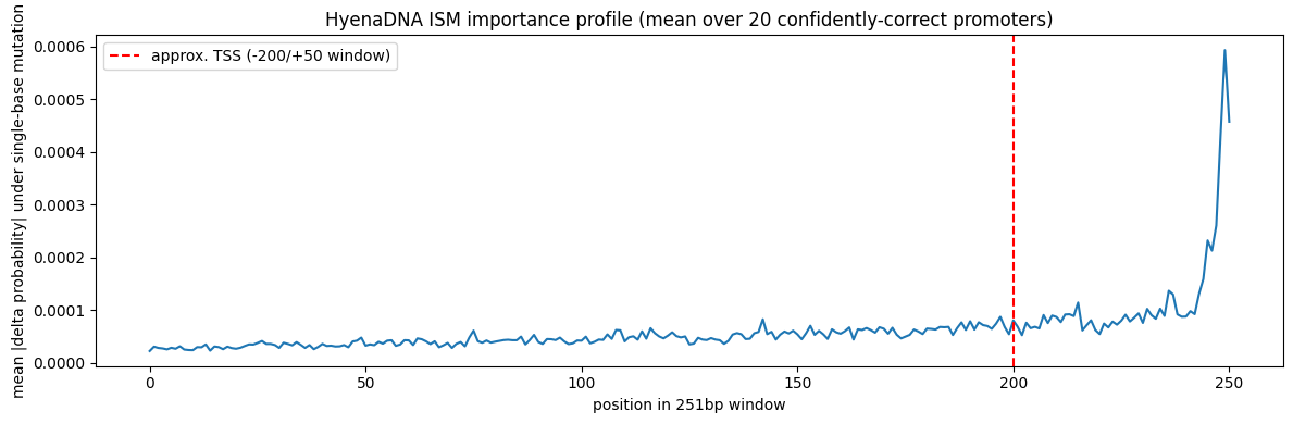
HyenaDNA has no attention mechanism (it's a convolutional architecture), so there are no attention weights to inspect. Interpretation instead used in-silico mutagenesis (ISM, notebooks/finetune_hyenadna.ipynb, interpretation section): for 20 confidently-correct positive test sequences, every position was mutated to each of the other 3 bases, and the resulting change in predicted promoter probability was recorded as that position's importance.
The initial result looked like it might be a tokenizer artifact: the highest-importance positions (245-250) sat at the extreme right edge of the 251bp window, not near the TSS (~200) as expected, and correlated weakly with GC/CpG content (0.18 / 0.27). Since sequences are padded to a fixed length for batching, this was checked directly by rerunning the identical ISM procedure with no padding at all: the result was unchanged (identical top-5 positions, near-identical curves), ruling out a padding-boundary artifact.
The actual explanation was found by reading modeling_hyena.py: HyenaDNAForSequenceClassification classifies using only the hidden state at the position of the last non-padding token (the same last-token pooling pattern used by GPT-2/Llama-style sequence classifiers). Because Hyena's mixing is causal, each position's hidden state only reflects itself and earlier positions, so the final token is the only one that has been exposed to the whole sequence. Positions near the end are structurally closest to that single read-out point, which mechanically inflates their measured importance regardless of true biological relevance. The importance profile's shape supports this: a slow, roughly flat baseline for most of the sequence, then a monotonically accelerating ramp into the last ~15 bases, not a localized bump at a specific position the way a real regulatory motif would look.
Negative-class control. The same ISM procedure was rerun on 20 confidently-correct negative sequences, which have no consistent biological landmark at their window edge, on the reasoning that if the edge effect is purely architectural it should appear in both classes equally. It did appear in both, confirming the positional artifact isn't promoter-specific, but the negative-class curve turned out to be 3-5x larger than the positive-class curve almost everywhere, not just at the edge: a second, unexpected confound. The selected positives sit at P(promoter) approx 0.98 and negatives at approx 0.03, both deep in the saturating tails of the softmax, so probability-space importance is compressed asymmetrically near the two extremes.
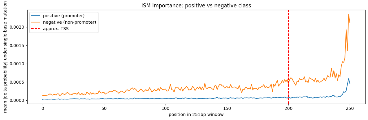
Margin-space control. Rerunning ISM in logit-margin space (the pre-softmax log-odds, which doesn't saturate) shrank the negative/positive importance ratio from 6.11 to 3.81, a real but partial effect: softmax saturation explains a meaningful part of the asymmetry, not all of it. The remainder likely reflects promoters being encoded more redundantly (many positions jointly support a strong, distributed compositional signal, so no single mutation moves the prediction much) than the negative class, whose "not a promoter" decision appears more sensitive to individual mutations. In both probability and margin space, subtracting the negative-class curve from the positive-class curve left a residual that is negative at every position, including near the TSS, not just at the edge: there is no position anywhere in the window where positive-class importance exceeds negative-class importance. The small TSS-proximal bump visible in the raw positive-only curve does not survive this control and shouldn't be read as a real signal.
ISM takeaway: naive position-wise ISM, in either probability or margin space, is dominated by two structural confounds for this model: proximity to the last-token pooling position, and a class-asymmetric sensitivity to mutation that isn't fully explained by softmax saturation. Neither the raw importance profile nor either background-corrected version provides evidence of a real, localized regulatory signal.
A different method: position-wise classification head readout. Every ISM variant measures perturbation sensitivity at the one pooled read-out point and inherits that point's biases no matter how the measurement is adjusted. HyenaDNAForSequenceClassification already computes self.score(hidden_states), the classification head, at every position internally before discarding all but the last one for pooling. Applying that same head, with the same trained weights, at every position directly (no mutation, a single forward pass) is a position-wise adaptation of the "logit lens" (Nostalgebraist, 2020, "Interpreting GPT: The Logit Lens", LessWrong), later formalized as the tuned lens by Belrose et al. (2023). The original technique reads intermediate layers through the final unembedding; HyenaDNA is only 2 layers deep, too shallow for that axis to be interesting, so this reads along the position axis instead, the exact axis the pooling confound was about. Because Hyena's mixing is causal, the hidden state at position i already reflects everything through position i, so this traces how the model's internal signal evolves as it processes the sequence, a direct look at accumulating evidence rather than a proxy for it.
Both classes start at nearly the same point (~+1.2 margin, minimal context) and dip together to about -1.3 by position 4-5. From there they diverge sharply and roughly monotonically over positions 5-100: positive climbs to about +3.6, negative falls to about -2.9. From position ~100 onward, spanning both the TSS (200) and the region ISM flagged as most important (245-250), both curves flatten into a plateau, adding almost no further evidence for the rest of the window.
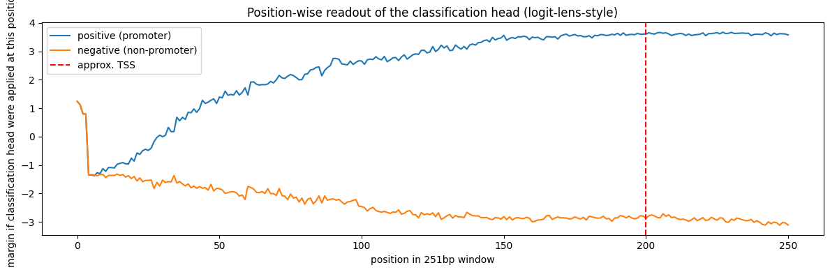
The per-position evidence increment (the localized quantity: how much new evidence position i+1 adds relative to position i) confirms this: the five positions where positive and negative increments diverge most are all clustered at positions 21-61 (roughly -179 to -139bp from the TSS), nowhere near the TSS or the tail.
This resolves the ISM confusion rather than just adding to it: the region ISM called "most important" is, by this more direct measurement, where the least new class-relevant information is incorporated. ISM was picking up proximity to the pooling read-out, exactly as the modeling_hyena.py mechanistic explanation predicted, now confirmed by an independent method that disagrees with ISM in precisely the way that explanation implies it should. Unlike ISM, this method surfaces a specific, plausible candidate signal: positions roughly 20-61 (upstream of the TSS), rather than nothing.
This finding is from a single run on 20 positive and 20 negative sequences and identifies where evidence accumulates, not what motif is there.
Motif cross-reference. Scanning the divergence zone (padded to positions 15-67) in the 20 positive sequences against JASPAR position-specific scoring matrices for five transcription factors documented at CpG-island, non-TATA promoters (both strands, best match per sequence) gives an uneven result across factors, not a uniform "everything matches" outcome:
| factor | best match in zone | expected by chance | mean best score | fraction of max |
|---|---|---|---|---|
| SP1 | 7/20 (35%) | 21% | 13.22 | 80% |
| KLF4 | 5/20 (25%) | 21% | 11.38 | 78% |
| YY1 | 4/20 (20%) | 21% | 3.03 | 21% |
| NRF1 | 2/20 (10%) | 22% | 8.68 | 43% |
| EGR1 | 1/20 (5%) | 21% | 9.66 | 58% |
SP1 is the standout: enriched above chance (35% vs 21%) and strong match quality (80% of the theoretical max score), consistent with SP1 being the textbook GC-box regulator of exactly this promoter type. EGR1 and NRF1 are actually below chance in this zone. YY1 sits at chance with weak absolute match quality (21% of max, essentially no real YY1 signal anywhere in these sequences). KLF4 is the interesting negative control: strong absolute match quality (78% of max, comparable to SP1) but only chance-level enrichment in the zone, meaning KLF4 sites are likely present but spread broadly across the sequence rather than concentrated there. That pattern is consistent with the earlier finding that raw GC/CpG composition correlates only weakly with the ISM importance profile (0.15-0.28): a generic GC-box-like signal doesn't localize to this zone, but SP1's more specific motif does.
This is exploratory (20 sequences, no multiple-testing correction, checking known motifs rather than discovering novel ones), but it gives the position-lens finding a specific, plausible biological identity rather than leaving it as an unexplained coordinate range.
tiny-1k-seqlen), chosen for free-tier compute feasibility, not the largest available.trust_remote_code=True.notebooks/finetune_hyenadna.ipynb self-contained: rebuilds the clean split, fine-tunes, evaluates, interprets
scripts/inspect_dataset.py class balance, sequence length, split-size inspection
scripts/check_leakage.py k-mer overlap audit (all sequences)
scripts/check_leakage2.py k-mer overlap audit (by class, by k)
scripts/build_clean_split.py rebuilds the leakage-free split, writes data/human_nontata_promoters_clean/
scripts/verify_clean_split.py confirms 0% exact/near-duplicate overlap on the rebuilt split
scripts/baseline_kmer_logreg.py k-mer frequency + logistic regression baseline
data/human_nontata_promoters_clean/ the rebuilt split (train.csv, test.csv)
figures/ key plots referenced in this README
Local scripts (dataset inspection, leakage checks, split rebuild, baseline) run in a Python 3.11 environment:
conda create -n genomic-finetune python=3.11
conda activate genomic-finetune
pip install datasets numpy pandas scikit-learn torch transformers
python scripts/build_clean_split.py
python scripts/verify_clean_split.py
python scripts/baseline_kmer_logreg.py
Fine-tuning and interpretation run in notebooks/finetune_hyenadna.ipynb on a free-tier Colab T4 GPU (Runtime > Change runtime type > T4 GPU, then run all cells). It's fully self-contained: no uploaded files needed.
Data and pretrained weights used in this project, and the papers behind the interpretation method:
human_nontata_promoters dataset.katarinagresova/Genomic_Benchmarks_human_nontata_promoters on the HuggingFace Hub.LongSafari on the HuggingFace Hub.MIT. See LICENSE for details.
This is a personal portfolio/learning project, but issues and pull requests are welcome, particularly around extending to other GenomicBenchmarks tasks (e.g. enhancer classification), or cross-referencing the position-lens candidate signal (positions ~20-61) against known CpG-island or transcription-factor motif annotations.
If you use this pipeline or reference its methodology, please cite:
Arunannamalai Sujatha Bharath Raj. (2026). Genomic Foundation Model Fine-tuning: HyenaDNA on Human Promoters. GitHub. https://github.com/Arun0364/genomic-finetune
For the underlying method and data, cite the original papers listed under References above.
Arun Sujatha Bharath Raj [email protected] | GitHub: @Arun0364
Built with Claude Code as a development tool.
Fine-tuning HyenaDNA on a promoter-vs-non-promoter classification task, evaluated against a simple k-mer baseline and interpreted with in-silico mutagenesis and a position-wise classification head readout.
Binary classification: is a 251bp human DNA sequence a non-TATA promoter, or a non-promoter fragment from a gene body?
Dataset: katarinagresova/Genomic_Benchmarks_human_nontata_promoters, part of the GenomicBenchmarks suite. Positive sequences span -200bp to +50bp around a transcription start site (TSS) lacking a TATA box; negatives are random 251bp fragments from human gene regions after the first exon. 36,131 sequences total, 54.4% positive.
Before trusting any result here, the train/test split was audited for the kind of batch effect that produces a suspicious, too-good-to-be-true accuracy. The official GenomicBenchmarks split for this dataset is a plain row-level sklearn.train_test_split(random_state=42) with no chromosome or locus grouping, confirmed directly from the dataset's construction notebook.
A k-mer overlap audit (scripts/check_leakage.py, scripts/check_leakage2.py) found:
scripts/build_clean_split.py rebuilds the split: sequences are clustered by shared 50-mers via union-find (any 50bp exact match implies overlapping loci), then whole clusters are assigned to train or test so no overlapping window crosses the split. scripts/verify_clean_split.py confirms 0% exact and 0% near-duplicate overlap on the result.
Clean split: 26,648 train / 9,483 test, 54.4% positive in both. Saved to data/human_nontata_promoters_clean/. All results below use this split, not the official one. Because of that, numbers here are not directly comparable to published GenomicBenchmarks leaderboard results on this dataset, and are expected to be somewhat lower, since the leaked split likely inflates reported accuracy.
The fine-tuning notebook rebuilds this same clean split from scratch at runtime (same algorithm, same seed), so it doesn't depend on the CSVs in data/ to reproduce.
LongSafari/hyenadna-tiny-1k-seqlen-hf: a 2-layer Hyena (implicit long-convolution) model, d_model=128, 436,352 total parameters, single-character tokenizer (4 nucleotides plus special tokens), max_seq_len=1026. Chosen for its small size and turnkey HuggingFace Trainer integration, making it realistic to fine-tune on free-tier compute.
Loading it requires trust_remote_code=True, which executes custom modeling/tokenizer code from the LongSafari HF repo rather than only transformers-native code. LongSafari is the paper authors' official org, but this is a different trust boundary than a fully first-party checkpoint and worth knowing before running the notebook.
The fine-tuned checkpoint is published at ArunBt64/hyenadna-tiny-nontata-promoters, so it can be loaded directly with AutoModelForSequenceClassification.from_pretrained("ArunBt64/hyenadna-tiny-nontata-promoters", trust_remote_code=True) rather than only reproduced via the notebook.
HuggingFace Trainer, batch size 32, learning rate 5e-5, best checkpoint selected by ROC-AUC. Run on a free-tier Colab T4 GPU: notebooks/finetune_hyenadna.ipynb.
An earlier run at a fixed 5 epochs showed clear overfitting past epoch 2 (training loss falling monotonically while validation loss rose the whole time). num_train_epochs is now set generously (10) with EarlyStoppingCallback(early_stopping_patience=1) on eval_roc_auc, so training stops itself shortly after ROC-AUC peaks rather than running the full budget. In practice this now stops after 3 epochs (epoch 3's ROC-AUC was worse than epoch 2's, exhausting the patience budget), restoring the epoch-2 checkpoint via load_best_model_at_end.
| metric | HyenaDNA (fine-tuned) | k-mer(6) + LogisticRegressionCV | delta |
|---|---|---|---|
| accuracy | 0.819 | 0.799 | +0.020 |
| precision | 0.845 | 0.894 | -0.049 |
| recall | 0.818 | 0.715 | +0.103 |
| F1 | 0.831 | 0.794 | +0.037 |
| ROC-AUC | 0.901 | 0.870 | +0.031 |
The baseline (scripts/baseline_kmer_logreg.py) uses 6-mer frequency vectors (4096-dim, per-sequence normalized) and LogisticRegressionCV(Cs=[0.01, 0.1, 1.0, 10.0, 100.0], cv=5, scoring="roc_auc"), which selected C=10, on the identical clean split.
HyenaDNA beats the baseline on accuracy, recall, F1, and ROC-AUC, but the baseline has higher precision. The baseline is more conservative (fewer false positives, more missed promoters), consistent with a bag-of-k-mers model catching only the most compositionally obvious cases while missing subtler ones that HyenaDNA's actual sequence modeling picks up. The margin is real but modest, not dramatic: this is a small model on a fairly compositionally-driven task (CpG-island promoters), so a k-mer baseline was always going to be a reasonably strong competitor.
HyenaDNA has no attention mechanism (it's a convolutional architecture), so there are no attention weights to inspect. Interpretation instead used in-silico mutagenesis (ISM, notebooks/finetune_hyenadna.ipynb, interpretation section): for 20 confidently-correct positive test sequences, every position was mutated to each of the other 3 bases, and the resulting change in predicted promoter probability was recorded as that position's importance.
The initial result looked like it might be a tokenizer artifact: the highest-importance positions (245-250) sat at the extreme right edge of the 251bp window, not near the TSS (~200) as expected, and correlated weakly with GC/CpG content (0.18 / 0.27). Since sequences are padded to a fixed length for batching, this was checked directly by rerunning the identical ISM procedure with no padding at all: the result was unchanged (identical top-5 positions, near-identical curves), ruling out a padding-boundary artifact.
The actual explanation was found by reading modeling_hyena.py: HyenaDNAForSequenceClassification classifies using only the hidden state at the position of the last non-padding token (the same last-token pooling pattern used by GPT-2/Llama-style sequence classifiers). Because Hyena's mixing is causal, each position's hidden state only reflects itself and earlier positions, so the final token is the only one that has been exposed to the whole sequence. Positions near the end are structurally closest to that single read-out point, which mechanically inflates their measured importance regardless of true biological relevance. The importance profile's shape supports this: a slow, roughly flat baseline for most of the sequence, then a monotonically accelerating ramp into the last ~15 bases, not a localized bump at a specific position the way a real regulatory motif would look.
Negative-class control. The same ISM procedure was rerun on 20 confidently-correct negative sequences, which have no consistent biological landmark at their window edge, on the reasoning that if the edge effect is purely architectural it should appear in both classes equally. It did appear in both, confirming the positional artifact isn't promoter-specific, but the negative-class curve turned out to be 3-5x larger than the positive-class curve almost everywhere, not just at the edge: a second, unexpected confound. The selected positives sit at P(promoter) approx 0.98 and negatives at approx 0.03, both deep in the saturating tails of the softmax, so probability-space importance is compressed asymmetrically near the two extremes.
Margin-space control. Rerunning ISM in logit-margin space (the pre-softmax log-odds, which doesn't saturate) shrank the negative/positive importance ratio from 6.11 to 3.81, a real but partial effect: softmax saturation explains a meaningful part of the asymmetry, not all of it. The remainder likely reflects promoters being encoded more redundantly (many positions jointly support a strong, distributed compositional signal, so no single mutation moves the prediction much) than the negative class, whose "not a promoter" decision appears more sensitive to individual mutations. In both probability and margin space, subtracting the negative-class curve from the positive-class curve left a residual that is negative at every position, including near the TSS, not just at the edge: there is no position anywhere in the window where positive-class importance exceeds negative-class importance. The small TSS-proximal bump visible in the raw positive-only curve does not survive this control and shouldn't be read as a real signal.
ISM takeaway: naive position-wise ISM, in either probability or margin space, is dominated by two structural confounds for this model: proximity to the last-token pooling position, and a class-asymmetric sensitivity to mutation that isn't fully explained by softmax saturation. Neither the raw importance profile nor either background-corrected version provides evidence of a real, localized regulatory signal.
A different method: position-wise classification head readout. Every ISM variant measures perturbation sensitivity at the one pooled read-out point and inherits that point's biases no matter how the measurement is adjusted. HyenaDNAForSequenceClassification already computes self.score(hidden_states), the classification head, at every position internally before discarding all but the last one for pooling. Applying that same head, with the same trained weights, at every position directly (no mutation, a single forward pass) is a position-wise adaptation of the "logit lens" (Nostalgebraist, 2020, "Interpreting GPT: The Logit Lens", LessWrong), later formalized as the tuned lens by Belrose et al. (2023). The original technique reads intermediate layers through the final unembedding; HyenaDNA is only 2 layers deep, too shallow for that axis to be interesting, so this reads along the position axis instead, the exact axis the pooling confound was about. Because Hyena's mixing is causal, the hidden state at position i already reflects everything through position i, so this traces how the model's internal signal evolves as it processes the sequence, a direct look at accumulating evidence rather than a proxy for it.
Both classes start at nearly the same point (~+1.2 margin, minimal context) and dip together to about -1.3 by position 4-5. From there they diverge sharply and roughly monotonically over positions 5-100: positive climbs to about +3.6, negative falls to about -2.9. From position ~100 onward, spanning both the TSS (200) and the region ISM flagged as most important (245-250), both curves flatten into a plateau, adding almost no further evidence for the rest of the window.
The per-position evidence increment (the localized quantity: how much new evidence position i+1 adds relative to position i) confirms this: the five positions where positive and negative increments diverge most are all clustered at positions 21-61 (roughly -179 to -139bp from the TSS), nowhere near the TSS or the tail.
This resolves the ISM confusion rather than just adding to it: the region ISM called "most important" is, by this more direct measurement, where the least new class-relevant information is incorporated. ISM was picking up proximity to the pooling read-out, exactly as the modeling_hyena.py mechanistic explanation predicted, now confirmed by an independent method that disagrees with ISM in precisely the way that explanation implies it should. Unlike ISM, this method surfaces a specific, plausible candidate signal: positions roughly 20-61 (upstream of the TSS), rather than nothing.
This finding is from a single run on 20 positive and 20 negative sequences and identifies where evidence accumulates, not what motif is there.
Motif cross-reference. Scanning the divergence zone (padded to positions 15-67) in the 20 positive sequences against JASPAR position-specific scoring matrices for five transcription factors documented at CpG-island, non-TATA promoters (both strands, best match per sequence) gives an uneven result across factors, not a uniform "everything matches" outcome:
| factor | best match in zone | expected by chance | mean best score | fraction of max |
|---|---|---|---|---|
| SP1 | 7/20 (35%) | 21% | 13.22 | 80% |
| KLF4 | 5/20 (25%) | 21% | 11.38 | 78% |
| YY1 | 4/20 (20%) | 21% | 3.03 | 21% |
| NRF1 | 2/20 (10%) | 22% | 8.68 | 43% |
| EGR1 | 1/20 (5%) | 21% | 9.66 | 58% |
SP1 is the standout: enriched above chance (35% vs 21%) and strong match quality (80% of the theoretical max score), consistent with SP1 being the textbook GC-box regulator of exactly this promoter type. EGR1 and NRF1 are actually below chance in this zone. YY1 sits at chance with weak absolute match quality (21% of max, essentially no real YY1 signal anywhere in these sequences). KLF4 is the interesting negative control: strong absolute match quality (78% of max, comparable to SP1) but only chance-level enrichment in the zone, meaning KLF4 sites are likely present but spread broadly across the sequence rather than concentrated there. That pattern is consistent with the earlier finding that raw GC/CpG composition correlates only weakly with the ISM importance profile (0.15-0.28): a generic GC-box-like signal doesn't localize to this zone, but SP1's more specific motif does.
This is exploratory (20 sequences, no multiple-testing correction, checking known motifs rather than discovering novel ones), but it gives the position-lens finding a specific, plausible biological identity rather than leaving it as an unexplained coordinate range.
tiny-1k-seqlen), chosen for free-tier compute feasibility, not the largest available.trust_remote_code=True.notebooks/finetune_hyenadna.ipynb self-contained: rebuilds the clean split, fine-tunes, evaluates, interprets
scripts/inspect_dataset.py class balance, sequence length, split-size inspection
scripts/check_leakage.py k-mer overlap audit (all sequences)
scripts/check_leakage2.py k-mer overlap audit (by class, by k)
scripts/build_clean_split.py rebuilds the leakage-free split, writes data/human_nontata_promoters_clean/
scripts/verify_clean_split.py confirms 0% exact/near-duplicate overlap on the rebuilt split
scripts/baseline_kmer_logreg.py k-mer frequency + logistic regression baseline
data/human_nontata_promoters_clean/ the rebuilt split (train.csv, test.csv)
figures/ key plots referenced in this README
Local scripts (dataset inspection, leakage checks, split rebuild, baseline) run in a Python 3.11 environment:
conda create -n genomic-finetune python=3.11
conda activate genomic-finetune
pip install datasets numpy pandas scikit-learn torch transformers
python scripts/build_clean_split.py
python scripts/verify_clean_split.py
python scripts/baseline_kmer_logreg.py
Fine-tuning and interpretation run in notebooks/finetune_hyenadna.ipynb on a free-tier Colab T4 GPU (Runtime > Change runtime type > T4 GPU, then run all cells). It's fully self-contained: no uploaded files needed.
Data and pretrained weights used in this project, and the papers behind the interpretation method:
human_nontata_promoters dataset.katarinagresova/Genomic_Benchmarks_human_nontata_promoters on the HuggingFace Hub.LongSafari on the HuggingFace Hub.MIT. See LICENSE for details.
This is a personal portfolio/learning project, but issues and pull requests are welcome, particularly around extending to other GenomicBenchmarks tasks (e.g. enhancer classification), or cross-referencing the position-lens candidate signal (positions ~20-61) against known CpG-island or transcription-factor motif annotations.
If you use this pipeline or reference its methodology, please cite:
Arunannamalai Sujatha Bharath Raj. (2026). Genomic Foundation Model Fine-tuning: HyenaDNA on Human Promoters. GitHub. https://github.com/Arun0364/genomic-finetune
For the underlying method and data, cite the original papers listed under References above.
Arun Sujatha Bharath Raj [email protected] | GitHub: @Arun0364
Built with Claude Code as a development tool.